Statistical Models to Estimate
Software Evolution Data From Repositories
By David A. Nader
Agenda
- Background
- terminology
- goal
- Exploratory Analysis
- Empirical Analysis
- Software Metrics
- Time Metrics
- Simulation
- ssq
- multi-server
- Original Traces
- Fitted
- non-stationary
Background
Software Repositories
- Issue: activity tracker (bug-req-task)
- Stakeholder: a person working for the project or issue
- Commit: tracking of changes of source code

Open
Close
Assigned
- Time Metrics
- issue-open: the creation of an issue
- issue-close: the timestamp of the finalization of an issue
- issue-wait: the difference between issue-open and issue-close
- issue-delay: the time of the issue before being assigned
- issue-service: the time of the issue after being assigned
- Software Management Metrics
- stakeholders: people involved in the issue realization
- effort: the measure of days-persons per issue-wait
Open
Close
Assigned
The goal of this project is to simulate the software evolution process from repositories meta-data
There are two approaches to this problem
- Simulation for Optimization 🡒 Software Management
- Simulation for Automation 🡒 Software Maintenance
Simulation for Optimization 🡒 Software Management
Three software engineering factors (Honsel, et al. 2014):
- Project Growth Trends
- Bug Appearance
- Development Strategies
Simulation for Optimization 🡒 Software Management
Three software engineering factors (Honsel, et al. 2014):
- Project Growth Trends
- Bug Appearance
- Developer Activity
Proposed Metrics:
- Project Growth Trends: Number of Commits
- Bug Appearance: Number of Issues (Jobs)
- Developer Activity: Effort
The goal of this project is to simulate the software evolution process from repositories meta-data to minimize the effort
Datasets

GHTorrent monitors the Github public event time line. For each event, it retrieves its contents and their dependencies, exhaustively. It then stores the raw JSON responses to a MongoDB database, while also extracting their structure in a MySQL database.

MSR2014 Challenge Dataset
This dataset includes data from the top-10 starred software projects for the top programming languages deployed in gitHub.
In total, there are 90 different projects with their respective derivations (forks).
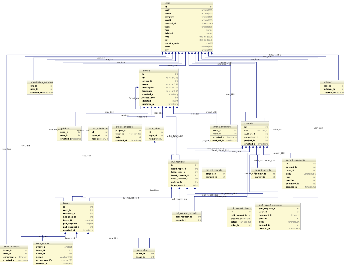
I utilized the datasets with the relational DB schema
Exploratory Analysis
- Analogies
- job: issue
- server: teams or software groups
- Time Metrics
- a_i: the creation of an issue
- c_i: the timestamp of the finalization of an issue
- w_i: the difference between issue-open and issue-close
- d_i: the time of the issue before being assigned
- s_i: the time of the issue after being assigned
- Software Management Metrics
- stakeholders: people involved in the issue realization
- effort: the measure of days-persons per issue-wait
- size: commits per trace
- Analogies
- job: issue
- server: teams or software groups
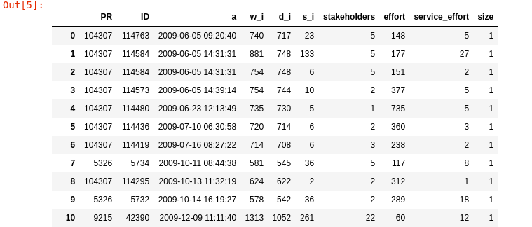
Software Evolution Trace Example - Timestamps
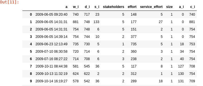
Computing Arrivals and Completions times

Exploratory Analysis of the Features
Cumulative Software Metrics
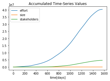
Stakeholders and Effort across the time
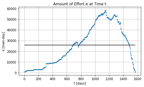
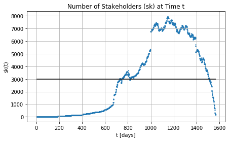
PDFs Arrivals and Services
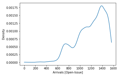
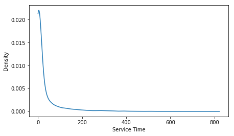
Fitted Arrivals and Services


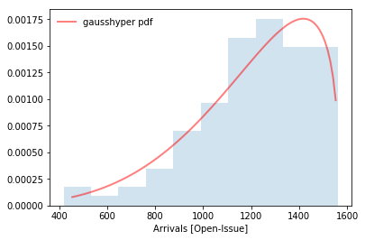
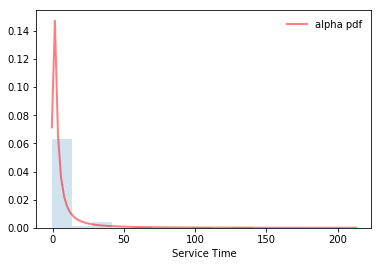
histograms main metrics

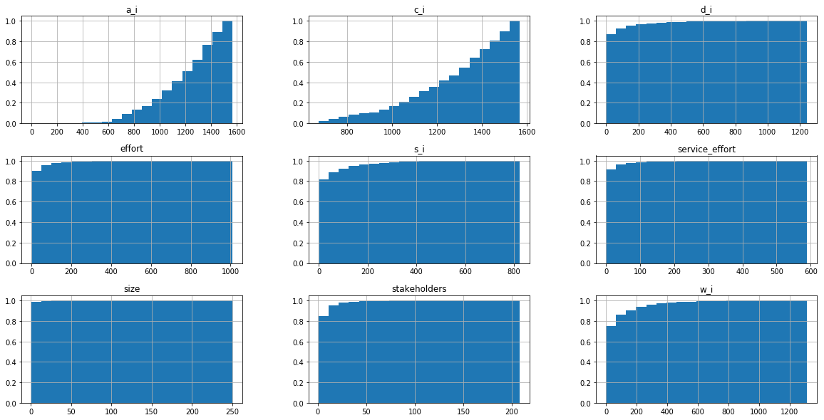
CDFs main metrics
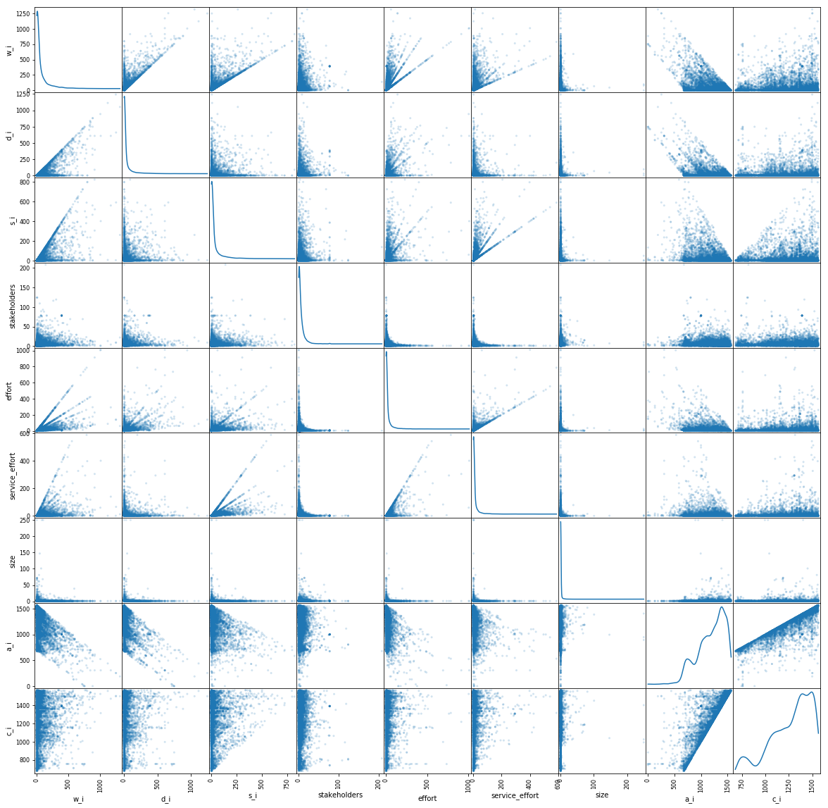
effort-w_i [r = 0.64]
effort-d_i: [r = 0.51]
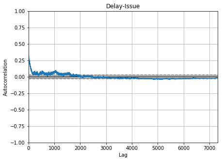
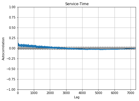
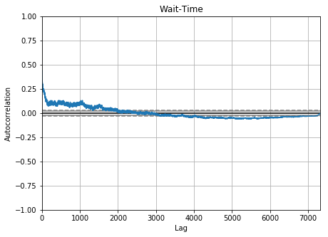
Auto-correlation in metrics of time

Empirical Analysis
Software and Time Metrics
First Order Statistics from Datasets
   average service time .... =  31.97
   average interarrival time =   0.21
   arrival rate ............ =   4.68
   average delay ........... =  32.35
   average wait ............ =  64.32
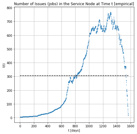
# of jobs in the node across the time
approx_servers:	         1176.58
approx_servers_max:	 38.29
number of servers?
approx_servers = max stakeholders across time / avg-stk
approx_servers_max = max stakeholders across time / max-stk
# of jobs in the Q across the time
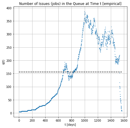
Time-Averaged Statistics
 avg # in node 	= 305.36
 avg # in queue = 155.9
 utilization 	= 149.46
Time-Averaged Statistics
 avg # in node 	= 305.36
 avg # in queue = 155.9
 utilization 	= 149.46
Consistency Metrics
avg wait 	= 64.32 64.32
avg # in node 	= 300.88 305.36
avg # in queue 	= 151.32 155.9
utilization 	= 149.55 149.46
Time-Averaged Statistics
 avg # in node 	= 305.36
 avg # in queue = 155.9
 utilization 	= 149.46
Consistency Metrics (Little's Law)
avg wait 	= 64.32 64.32
avg # in node 	= 300.88 305.36
avg # in queue 	= 151.32 155.9
utilization 	= 149.55 149.46
Approx Utilization per server
avg utilization[server] 	= 0.13
max utilization[server] 	= 3.91
Simulation
ssq
Simulating with
for 7326 jobs
   average interarrival time =   0.21
   average service time .... =  31.97
   average delay ........... = 22838.20
   average wait ............ = 22870.17
Simulating with
for 7326 jobs
   average interarrival time =   0.21
   average service time .... =  31.97
   average delay ........... = 22838.20
   average wait ............ = 22870.17
   average service time .... =  31.97
   average interarrival time =   0.21
   arrival rate ............ =   4.68
   average delay ........... =  32.35
   average wait ............ =  64.32
Simulating with
for 7326 jobs
   average interarrival time =   0.21
   average service time .... =  31.97
   average delay ........... = 22838.20
   average wait ............ = 22870.17
Approximation Error
   avg wait error ............ 	= 354.59
   avg delay error ............ 	= 705.04
   avg interarrival error ............ 	=   0.00
   avg service error ............ 	=   0.00
   average service time .... =  31.97
   average interarrival time =   0.21
   arrival rate ............ =   4.68
   average delay ........... =  32.35
   average wait ............ =  64.32
multi-server
Simulating with msq providing arrivals and exponential service times with 150 servers
for 7325 jobs and 150 servers the service node statistics (for 35 runs) are:
  avg interarrivals .. =   0.21
  avg wait ........... = 283.65
  avg # in node ...... = 864.21
  avg delay .......... = 251.73
  avg # in queue ..... = 766.94
  sim utilization	= 97.26
  sim service	= 32.54
Confidence Values [c=0.95]
  avg interarrivals .. = [0.21 0.21 0.21]
  avg wait ........... = [283.97 280.97 286.97]
  avg # in node ...... = [864.23 855.9  872.55]
  avg delay .......... = [251.98 249.09 254.86]
  avg # in queue ..... = [766.86 758.82 774.9 ]
  sim utilization	= [97.37 96.94 97.79]
  sim service	= [32.64 32.5  32.78]
Avg. Approximation Error for msq
| metric | with exponential services | ... |
|---|---|---|
| avg wait | 3.42 | |
| avg delay | 6.79 | |
| avg interarrival | 0.00 | |
| avg service | 0.02 | |
| utilization | 0.35 | |
| avg # in node | 1.87 | |
| avg # in q | 4.07 |
Avg. Approximation Error for msq providing fitted time services
| metric | with exponential services | with fitted services |
|---|---|---|
| avg wait | 3.42 | 0.87 |
| avg delay | 6.79 | 1.00 |
| avg interarrival | 0.00 | 0.00 |
| avg service | 0.02 | 0.73 |
| utilization | 0.35 | 0.77 |
| avg # in node | 1.87 | 0.89 |
| avg # in q | 4.07 | 1.00 |
Avg. Approximation Error for msq providing fitted services and non-stationary arrivals (thinning method)
| metric | with exponential services | with fitted services | with fitted services and non stationary arrivals (λ_max) |
|---|---|---|---|
| avg wait | 3.42 | 0.87 | 0.87 |
| avg delay | 6.79 | 1.00 | 1.00 |
| avg interarrival | 0.00 | 0.00 | 3.70 |
| avg service | 0.02 | 0.73 | 0.74 |
| utilization | 0.35 | 0.77 | 0.95 |
| avg # in node | 1.87 | 0.89 | 0.97 |
| avg # in q | 4.07 | 1.00 | 1.00 |
Avg. Approximation Error for msq providing non-stationary arrivals and exponential services
| metric | with exponential services | with fitted services | with fitted services and non stationary arrivals (λ_max) | with exponential services and non stationary arrivals (λ_max) |
|---|---|---|---|---|
| avg wait | 3.42 | 0.87 | 0.87 | 0.50 |
| avg delay | 6.79 | 1.00 | 1.00 | 1.00 |
| avg interarrival | 0.00 | 0.00 | 3.70 | 3.70 |
| avg service | 0.02 | 0.73 | 0.74 | 0.02 |
| utilization | 0.35 | 0.77 | 0.95 | 0.80 |
| avg # in node | 1.87 | 0.89 | 0.97 | 0.90 |
| avg # in q | 4.07 | 1.00 | 1.00 | 1.00 |
Simulating with msq providing arrivals and exponential service times with approx. servers
for 7325 jobs and 1176 servers the service node statistics (for 35 runs) are:
  avg interarrivals .. =   1.00
  avg wait ........... =  31.85
  avg # in node ...... =  29.19
  avg delay .......... =   0.00
  avg # in queue ..... =   0.00
  sim utilization	= 29.19
  sim service	= 32.2
Confidence Values [c=0.95]
  avg interarrivals .. = [1. 1. 1.]
  avg wait ........... = [31.85 31.58 32.12]
  avg # in node ...... = [29.19 28.87 29.52]
  avg delay .......... = [ 0. -0.  0.]
  avg # in queue ..... = [ 0. -0.  0.]
  sim utilization	= [29.19 28.87 29.52]
  sim service	= [32.2 31.9 32.5]
Avg. Approximation Error for msq providing non-stationary arrivals and exponential services
| metric | with exponential services | with fitted services | with fitted services and non stationary arrivals (λ_max) | with exponential services and non stationary arrivals (λ_max) | with approx servers |
|---|---|---|---|---|---|
| avg wait | 3.42 | 0.87 | 0.87 | 0.50 | 0.50 |
| avg delay | 6.79 | 1.00 | 1.00 | 1.00 | 1.00 |
| avg interarrival | 0.00 | 0.00 | 3.70 | 3.70 | 3.69 |
| avg service | 0.02 | 0.73 | 0.74 | 0.02 | 0.01 |
| utilization | 0.35 | 0.77 | 0.95 | 0.80 | 0.80 |
| avg # in node | 1.87 | 0.89 | 0.97 | 0.90 | 0.90 |
| avg # in q | 4.07 | 1.00 | 1.00 | 1.00 | 1.00 |
Summary

Simulation for Optimization 🡒 Software Management

Simulation for Optimization 🡒 Software Management

Accumulated Effort Across the Time

Simulation for Optimization 🡒 Software Management

Accumulated Effort Across the Time
effort-w_i [r = 0.64]
effort-d_i: [r = 0.51]
Effort vs {w_i, d_i}

Simulation for Optimization 🡒 Software Management

Accumulated Effort Across the Time
effort-w_i [r = 0.64]
effort-d_i: [r = 0.51]
| metric | with exponential services | with fitted services | with fitted services and non stationary arrivals (λ_max) | with exponential services and non stationary arrivals (λ_max) | with approx servers |
|---|---|---|---|---|---|
| avg wait | 3.42 | 0.87 | 0.87 | 0.50 | 0.50 |
| avg delay | 6.79 | 1.00 | 1.00 | 1.00 | 1.00 |
| avg interarrival | 0.00 | 0.00 | 3.70 | 3.70 | 3.69 |
| avg service | 0.02 | 0.73 | 0.74 | 0.02 | 0.01 |
| utilization | 0.35 | 0.77 | 0.95 | 0.80 | 0.80 |
| avg # in node | 1.87 | 0.89 | 0.97 | 0.90 | 0.90 |
| avg # in q | 4.07 | 1.00 | 1.00 | 1.00 | 1.00 |
Avg. Approx. Error
Effort vs {w_i, d_i}
State-of-the-art
Previous research can be classified into two categories
- Simulations about Software Engineering
- Data-mining techniques on the MSE2014 dataset
Simulations about Software Engineering (2014)


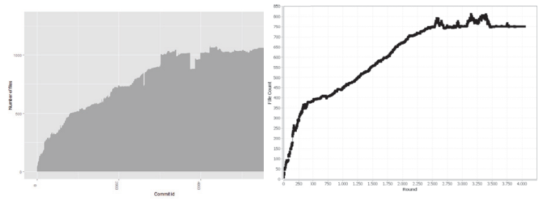
Simulations about Software Engineering (2015)


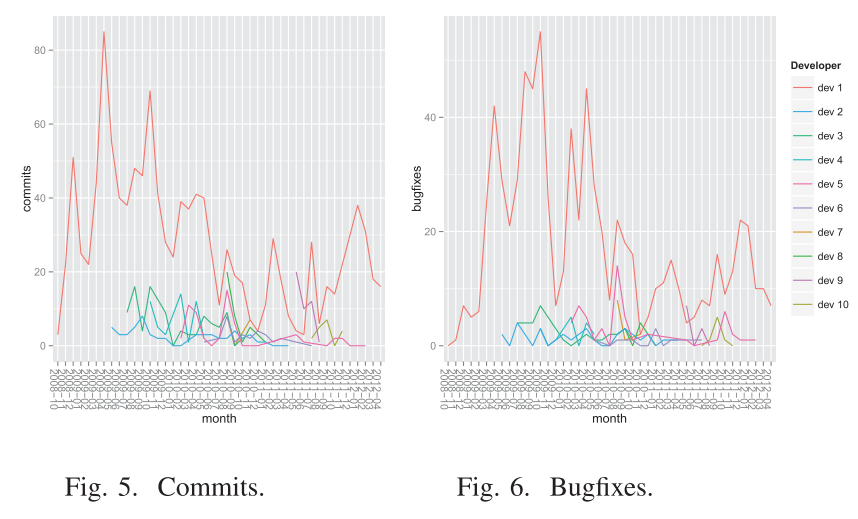

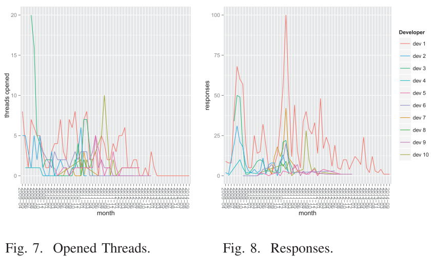
Simulations about Software Engineering (2018)


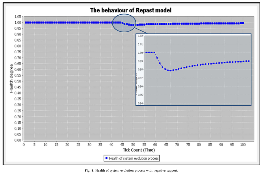
Data-mining techniques on the MSE2014 dataset

Data-mining techniques on the MSE2014 dataset


Data-mining techniques on the MSE2014 dataset


Data-mining techniques on the MSE2014 dataset


create or replace view v_processed_issues as select FirstSet.PR, FirstSet.ID,
		FirstSet.open_issue,
        FirstSet.wait_issue,
        SecondSet.delay_issue,
		(FirstSet.wait_issue-SecondSet.delay_issue) as service_issue,
        ThirdSet.stakeholders,
		ceil(FirstSet.wait_issue/ThirdSet.stakeholders) as effort,
        ceil((FirstSet.wait_issue-SecondSet.delay_issue)
            /ThirdSet.stakeholders) as service_effort
from
	(select distinct ISU.id as ID, ISU.repo_id as PR,
	ISU.created_at as open_issue, ISUE.action as AC,
	TIMESTAMPDIFF(DAY, ISU.created_at, ISUE.created_at) as wait_issue
	from msr14.issues as ISU join msr14.issue_events as ISUE on ISU.id = ISUE.issue_id
    where ISUE.action='closed') as FirstSet
inner join
	(select distinct ISU.id as ID, ISU.repo_id as PR,
	ISU.created_at as open_issue, ISUE.action as AC,
	TIMESTAMPDIFF(DAY, ISU.created_at, ISUE.created_at) as delay_issue
	from msr14.issues as ISU join msr14.issue_events as ISUE on ISU.id = ISUE.issue_id
    where ISUE.action='assigned') as SecondSet
on FirstSet.PR = SecondSet.PR and FirstSet.ID = SecondSet.ID
inner join v_issues as ThirdSet
on FirstSet.ID = ThirdSet.IS_ID
having service_issue >= 0
and FirstSet.wait_issue >= 0
and SecondSet.delay_issue >= 0
order by FirstSet.open_issue;
An sql view to create the "Software Evolution Traces"

There are 90 different SW projects
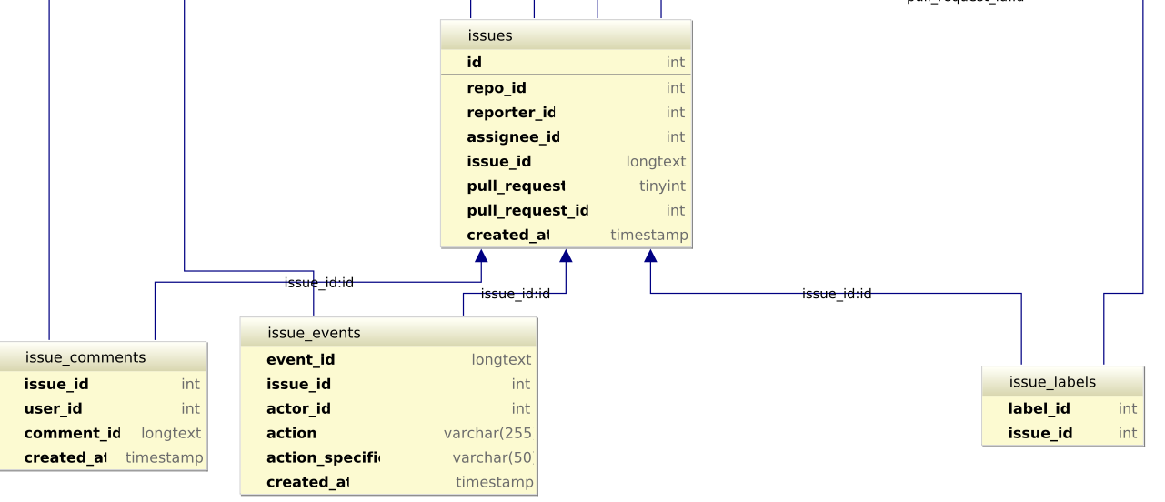
One project has multiple issues

A pull-request has multiple issues