Active inference with semi-Markov models

Active Inference with Semi-markov models

Dimitrije Marković

Theoretical Neurobiology Meeting

01.03.2020

Active inference and semi-markov decision processes

(Part I) Active inference in multi-armed bandits
- Empirical comparison with UCB and Thompson sampling.
- https://slides.com/dimarkov/ai-mbs

(Part II) Active inference and semi-Markov processes
- Hidden semi-Markov models and a representation of state duration.
- Learning the hidden temporal structure of state transitions.
- Application: Reversal learning task.
(Part III) Active inference and semi-Markov decision processes
- Extending policies with action (policy) duration.
- Decision about when actions should be taken and for how long.
- Applications: Temporal attention, intertemporal choices.

Active inference and semi-markov decision processes

(Part I) Active inference in multi-armed bandits
- Empirical comparison with UCB and Thompson sampling.
- https://slides.com/dimarkov/ai-mbs

(Part II) Active inference and semi-Markov processes
- Hidden semi-Markov models and a representation of state duration.
- Learning the hidden temporal structure of state transitions.
- Application: Reversal learning task.
(Part III) Active inference and semi-Markov decision processes
- Extending policies with action (policy) duration.
- Decision about when actions should be taken and for how long.
- Applications: Temporal attention, intertemporal choices.

(Part II) Active inference and semi-Markov processes
- Hidden semi-Markov models and a representation of state duration.
- Learning the hidden temporal structure of state transitions.
- Application: Reversal learning task.

Semi-Markov processes

https://en.wikipedia.org/wiki/Markov_renewal_process#Relation_to_other_stochastic_processes

State space S
Jump times \(T_n\) and states \( X_n\)
Inter-arrival time \( \tau_n = T_n - T_{n-1}\)
The sequence \( [(X_0, T_0), \ldots, (X_n, T_n), \ldots]\) is called a Markov renewal process if:

Pr\left(\tau_n \leq t, X_{n}=j| (X_0, T_0), \ldots, (X_{n-1}=i, T_n) \right) = Pr\left(\tau_n \leq t, X_{n}=j| X_{n-1}=i \right)

If \( Y_t \equiv X_n \) for \( t \in \left[T_n, T_{n+1} \right)\) then the process \(Y_t\) is called a semi-Markov process

Semi-Markov processes

State space \( S\)

X_0

X_1

X_2

X_{n-1}

X_n

X_{n+1}

\( \ldots\)

T_0

T_1

T_2

T_{n-1}

T_{n}

T_{n+1}

Time

\tau_1

\tau_2

\tau_n

\tau_{n+1}

Special cases

For exponentially distributed iid waiting times we have a continuous time Markov chain

Pr\left(\tau_n \leq t, X_{n}=j| X_{n-1}=i \right) = Pr\left(X_{n}=j| X_{n-1}=i \right) \left( 1 - e^{\lambda_i t} \right)

A discrete time Markov chain has geometrically distributed waiting times

Pr\left(X_{n}=i| X_{n-1}=i \right) = p_i

\tau_n \sim p(\tau|p_i) = p_i^{\tau - 1}(1 - p_i), \:\: \tau \in \{1, 2, 3, \ldots\}

Hidden Semi-Markov models

Shun-Cheng Yu, "Hidden semi-Markov Models: Theory, Algorithms and Applications", Elsevir 2016.

https://doi.org/10.1016/C2014-0-02508-7

A graphical representation of HSMM

Latent variables

outcomes

f_t

s_t

o_t

f_{t-1}

f_{t+1}

s_{t-1}

s_{t+1}

o_{t-1}

o_{t+1}

Example

\( f \in \{1, 2, 3\}\)

\tau = 3

time step

\( s \in \{A, B\}\)

\tau = 5

\tau = 2

p(f_t|f_{t-1}, s_{t-1}) \equiv \tau \sim p(\tau|s)

Example

\( f \in \{1, 2, 3\}\)

\tau = 3

time step

\( s \in \{A, B\}\)

\tau = 5

\tau = 2

p(f_t|f_{t-1}) \equiv \tau \sim p(\tau)

Phase transitions

\[p(f_t|f_{t-1})\]

M Varmazyar, et al., Journal of Industrial Engineering International (2019).

Discrete phase-type distribution

\omega_i = {n \choose i-1} (1 - \delta)^{n - i + 1}\delta^{i-1}, \:\: \omega_0 = 1 - \sum_{i=1}^{n} \omega_i

1-\delta

\delta

n+1

\(\ldots\)

\omega_1

\omega_2

\omega_{n}

\omega_{0}

Phase transitions

\[p(f_t|f_{t-1})\]

M Varmazyar, et al., Journal of Industrial Engineering International (2019).

Discrete phase-type distribution

Duration distribution

Negative binomial

\[p(\tau) = {\tau + n - 2 \choose \tau-1}(1-\delta)^{\tau-1}\delta^n\]

E[\tau]=\frac{n (1-\delta)}{\delta}+1 = \mu + 1

Var[\tau] = \mu + \frac{\mu^2}{n}

\omega_i = {n \choose i-1} (1 - \delta)^{n - i + 1}\delta^{i-1}, \:\: \omega_0 = 1 - \sum_{i=1}^{n} \omega_i

1-\delta

\delta

n+1

\(\ldots\)

\omega_1

\omega_2

\omega_{n}

\omega_{0}

Phase transitions

\[p(f_t|f_{t-1})\]

State transitions

\( p(s_t|s_{t-1}, f_{t-1})\)

1-\delta

\delta

n+1

\(\ldots\)

\omega_1

\omega_2

\omega_{n}

\omega_{0}

negative binomial distribution

\delta_d = p(s_{t+d}=B|s_t=A)

Active Inference

p\left(o_t^l| s_t^1, \ldots, s_t^K\right) = Cat\left( A^l \right)

p\left(A^l\right) = Dir(a^l)

p\left(s_t^k| s_{t-1}^k, \pi, f_t \right) = Cat\left( B^{k, \pi}_f \right)

p(\pi) = s_{max}\left( -\gamma G \right), \quad P(o^l_t) = s_{max} \left( C^l \right)

p\left(f_t| f_{t-1}, m \right) = Cat\left( L^{m} \right)

p(m) = Cat(M), \quad m = (\mu, n)

\mu \in \{ \mu_{min}, \ldots, \mu_{max} \}, \: n \in \{1, \ldots, n_{max}\}

s^1_{t-1}

s^1_{t}

A^l

o_t

B^k

\pi

f_{t-1}

f_{t}

Belief updating and learning

History of past outcomes \( O_t = (o_1, \ldots, o_t) \)

Q(m) \propto p(o_t|m, O_{t-1}) p(m|O_{t-1})

Q(f_t|m) \propto p(o_t|f_t, O_{t-1}) p(f_t|m, O_{t-1})

Q(s_t|f_t) \propto p(o_t|s_t) e^{\sum_{\pi} Q(\pi) \ln p\left(s_t|f_t, \pi, O_{t-1} \right)}

Q(\pi) \propto p(o_t|\pi, O_{t-1}) p(\pi|O_{t-1})

Q(A) \propto e^{\sum_{s_t} Q(s_t) \ln p(o_t|s_t, A)} P(A|O_{t-1})

p(o_t| x, O_{t-1}) = \sum_y p(o_t|y) p(y|x, O_{t-1})

p(x_t|O_{t-1}) = \sum_{x_{t-1}} p(x_t|x_{t-1}) Q(x_{t-1})

Marginal likelihood

Predictive prior

Action selection

u_t \sim p\left(\pi|O_{t-1}\right) \propto e^{-\gamma G(\pi)}

When simulating behaviour \( \gamma \rightarrow \infty \)

For data analysis \( \gamma \) is a free parameter

G(\pi) = E_{Q(o_t|\pi)}\left[ \ln \frac{Q(o_t|\pi)}{P(o_t)} \right] - E_{Q(o_t, s_t, A|\pi)} \left[ \ln p(o_t|s_t, A) \right]

Probabilistic reversal learning

Model parameters

\( f \in \{1, \ldots, n_{max} \} \)

\( \otimes \)

loss

gain

cue A

cue B

\(P(o_t^1) = [\frac{1}{3}, \frac{1}{3}, \frac{1}{3}] \)

\(P(o_t^2) = [\rho_1, \rho_2, \frac{\rho}{2}, \frac{\rho}{2}] \)

Performance

\frac{MA(t)}{1 - MA(t)}

Trials Until correct (TUC)

In SILICO

Is the experimental setup useful?

Can the temporal structure be learned?
Will different temporal beliefs reflect different behaviour?
How well can we differentiate between agents with different temporal beliefs?

In SILICO

Process:

Fix priors, and action precision \(\gamma\)
Simulate behaviour in both conditions with different \(n_{max}\)
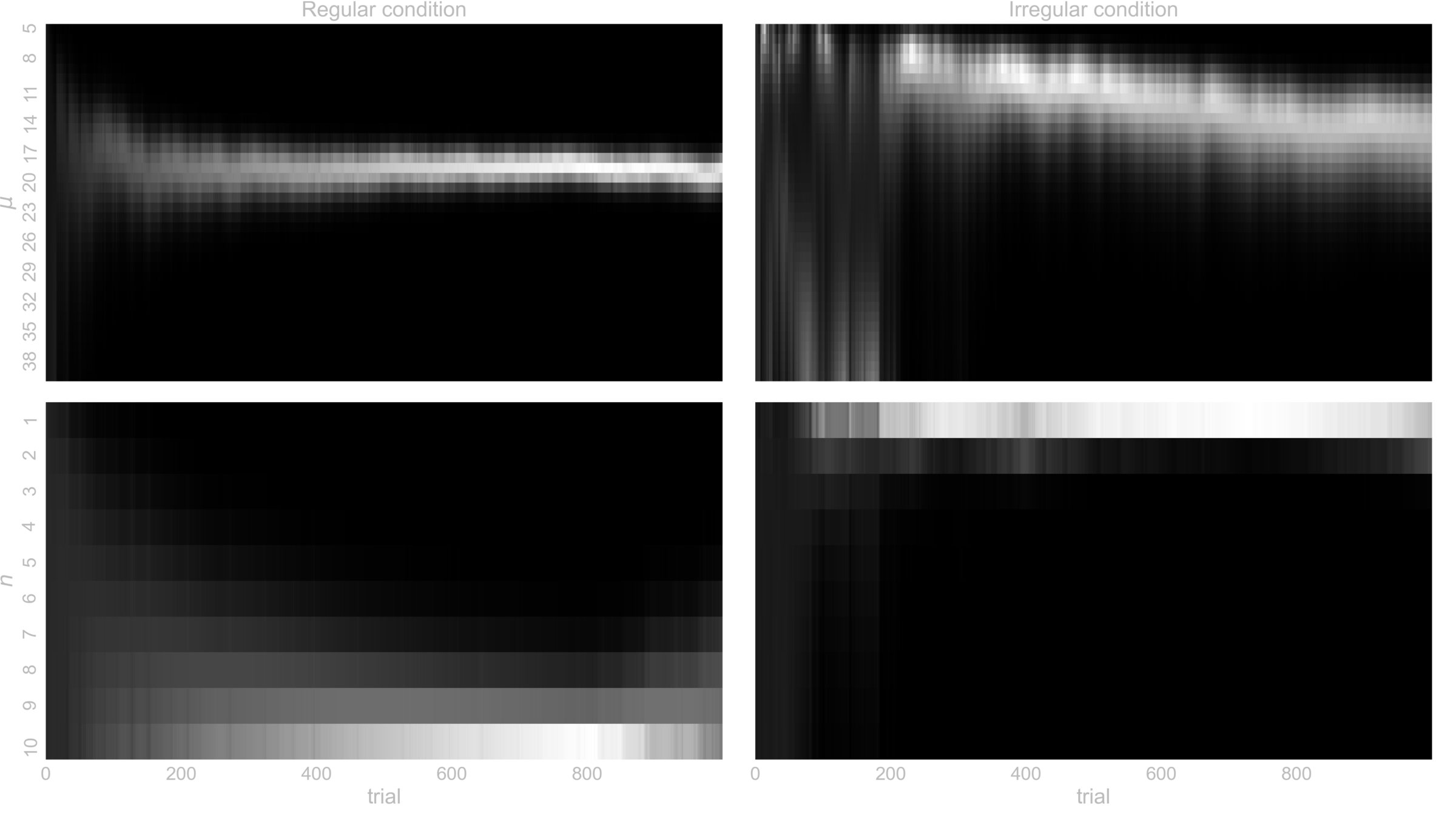
Illustrate, performance, TUC, and the learning of the latent temporal structure \( (\mu, n) \)
Model inversion, and confusion matrix for \(n_{max}\)

In SILICO - Behavioural metrics

In SILICO - Learning latent temporal structure

n_{max} = 10

In SILICO - Confusion matrix

Behavioural data

50 healthy volunteers (20-30 years old):
- 27 subjects in the condition with regular reversals
- 23 subjects in the condition with irregular reversals
40 trials long training with a single reversal

Performance-tuc trajectories

Model comparison

Labeled trajectories

conclusion

Modelling and assessing influence of temporal-expectations on decision-making in dynamic environments.

How people learn temporal expectations could also be addressed with this approach, but some challenges remain.

Linking the underlying representation of the temporal structure to behaviour provides a novel method for computational cognitive phenotyping.

Thanks to:

Andrea Reiter
Stefan Kiebel
Thomas Parr
Karl Friston

https://slides.com/dimarkov/active-inference-semi-markov

https://github.com/dimarkov/pybefit

https://journals.plos.org/ploscompbiol/article?rev=2&id=10.1371/journal.pcbi.1006707