Bayesian sparse regression

Dimitrije Marković

DySCO meeting 16.02.2022

Sparse regression in GLMs

\mu_k = \alpha + \sum_{d=1}^D \beta_d x_{d, k} \\ \mu_k = \alpha + \pmb{X}_k \cdot \pmb{\beta} \\ y_k \sim p(y_k|\mu_k, \theta);\:\: \text{for } k \in \{1, \ldots, N\}

Sparse regression in GLMs

Outline

Bayesian regression
Hierarchical priors
Shrinkage priors
QR decomposition
Pairwise interactions

Linear regression model

\mu_k = \alpha + \sum_{d=1}^D \beta_d x_{d, k} \\ y_k = \mu_k + \epsilon_k \\ \epsilon_k \sim \mathcal{N}(0, \sigma)

D = 50, N = 200 \\ \alpha = 0, \quad X_k \sim \mathcal{N} \left(0, \pmb{I}_D\right) \\ \beta_{1}, \ldots, \beta_{S} > 0; \quad \beta_{d>S} = 0; \quad S=5 \\ \sigma = 1.

Simulated data

Generative model

p \left(y | \pmb{X}, \pmb{\beta}, \sigma \right) = \mathcal{N} \left(y; \pmb{X} \cdot \pmb{\beta}, \sigma^2 \right) \\ p(\pmb{\beta}) = \mathcal{N}_D\left(\pmb{\beta}; 0, \sigma^2 \tau^2 \pmb{\Lambda} \right) \\ \pmb{\Lambda} = diag(\lambda_1^2, \ldots, \lambda_D^2) \\ \mathcal{D} = \left( \pmb{X}, \pmb{y} \right)

Posterior distribution

p\left(\pmb{\beta}|\pmb{\Lambda}, \tau, \sigma, \mathcal{D} \right) = \mathcal{N}\left(\pmb{\beta}; \bar{\pmb{\beta}}, \pmb{\Sigma} \right) \\ \hat{\pmb{\beta}} = \left( \pmb{X}^T \pmb{X} \right)^{-1} \pmb{X}^T \pmb{y} \\ \bar{\pmb{\beta}} = \tau^2 \pmb{\Lambda} \left( \tau^2 \pmb{\Lambda} + \left(\pmb{X}^T \pmb{X} \right)^{-1} \right)^{-1} \hat{\pmb{\beta}}\\ \pmb{\Sigma} = \sigma^2 \left( \frac{1}{\tau^2} \pmb{\Lambda}^{-1} + \pmb{X}^T \pmb{X} \right)^{-1}

\sigma = 1, \quad \pmb{\Lambda} = \pmb{I}_D, \quad \pmb{X}^T\cdot \pmb{X} \approx N \pmb{I}_D

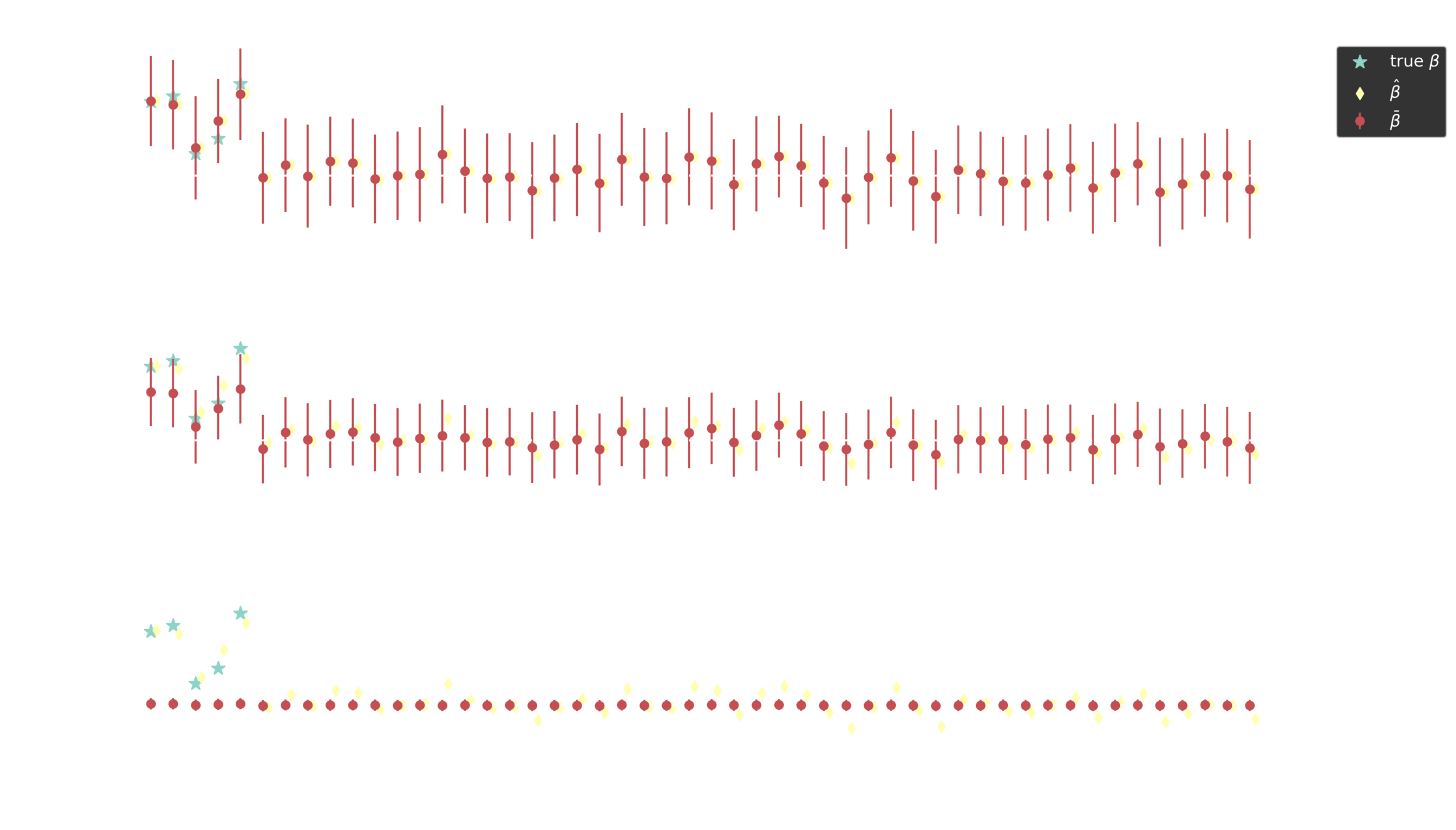
Posterior estimates

Shrinkage factor

Var\left( \pmb{x}_d \right) = s_d, \quad \pmb{X}^T\cdot \pmb{X} \approx N \pmb{I}_D

\bar{\beta}_d = (1 - \kappa_d) \hat{\beta}_d

\kappa_d = \frac{1}{1 + N \tau^2 \lambda_d^2 s_d}

Piironen, Juho, and Aki Vehtari. "Sparsity information and regularization in the horseshoe and other shrinkage priors." Electronic Journal of Statistics 11.2 (2017): 5018-5051.

Generative model

p \left(y | \pmb{X}, \pmb{\beta}, \sigma \right) = \mathcal{N} \left(y; \alpha + \pmb{X} \cdot \pmb{\beta}, \sigma^2 \right) \\ p(\pmb{\beta}) = \mathcal{N}_D\left(\pmb{\beta}; 0, \sigma^2 \tau^2 \pmb{\Lambda} \right) \\ \pmb{\Lambda} = diag(\lambda_1^2, \ldots, \lambda_D^2) \\ p(\alpha) = \mathcal{N}(0, 10) \\ p\left( \sigma^2 \right) = \Gamma^{-1} \left(2, 2 \right) \\ \mathcal{D} = \left( \pmb{X}, \pmb{y} \right)

Posterior estimates

Horseshoe prior

\kappa_d = \frac{1}{1 + N \tau^2 \lambda_d^2 s_d}

Piironen, Juho, and Aki Vehtari. "Sparsity information and regularization in the horseshoe and other shrinkage priors." Electronic Journal of Statistics 11.2 (2017): 5018-5051.

\lambda_d \sim C^+(0, 1)

Half-Cauchy distribution

Hierarchical generative model

p\left( \sigma^2 \right) = \Gamma^{-1} \left(2, 2 \right) \\ p\left( \lambda_d \right) = C^+(0, 1) \\ p(\beta_d|\lambda_d) = \mathcal{N}\left(0, \sigma^2 \tau^2 \lambda_d^2 \right) \\ p(\alpha) = \mathcal{N}(0, 10) \\ p \left(y | \pmb{X}, \pmb{\beta}, \sigma \right) = \mathcal{N} \left(y; \alpha + \pmb{X} \cdot \pmb{\beta}, \sigma^2 \right)

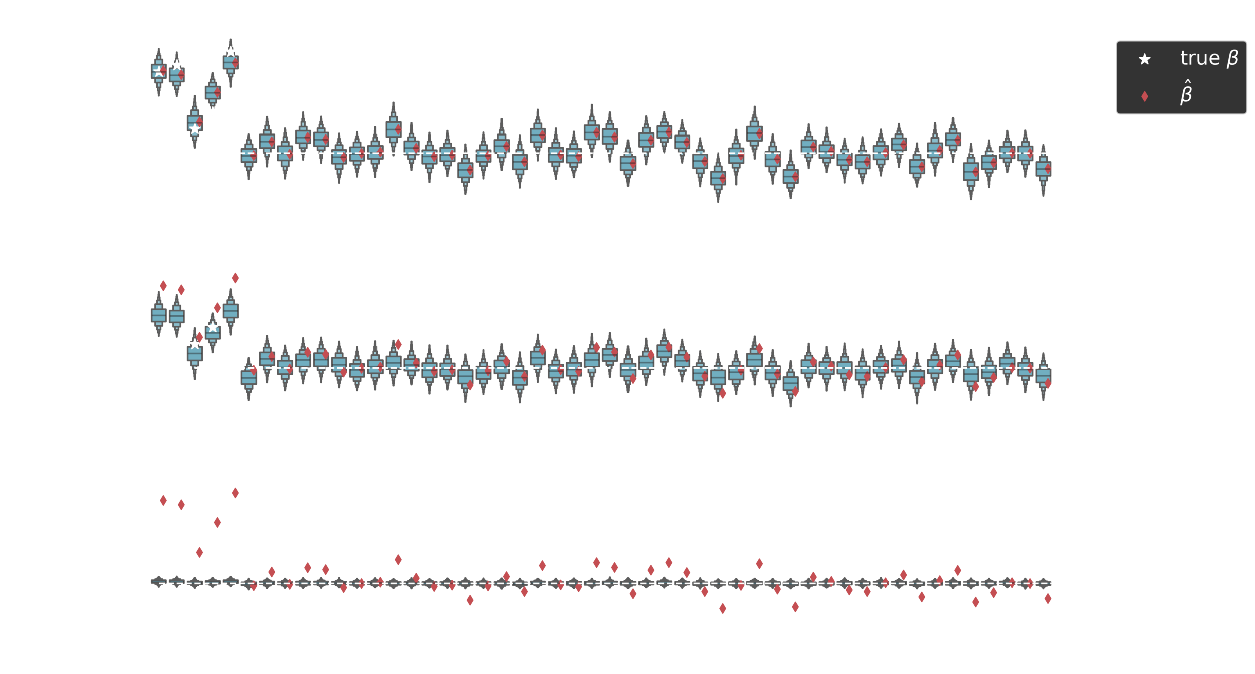
Posterior estimates

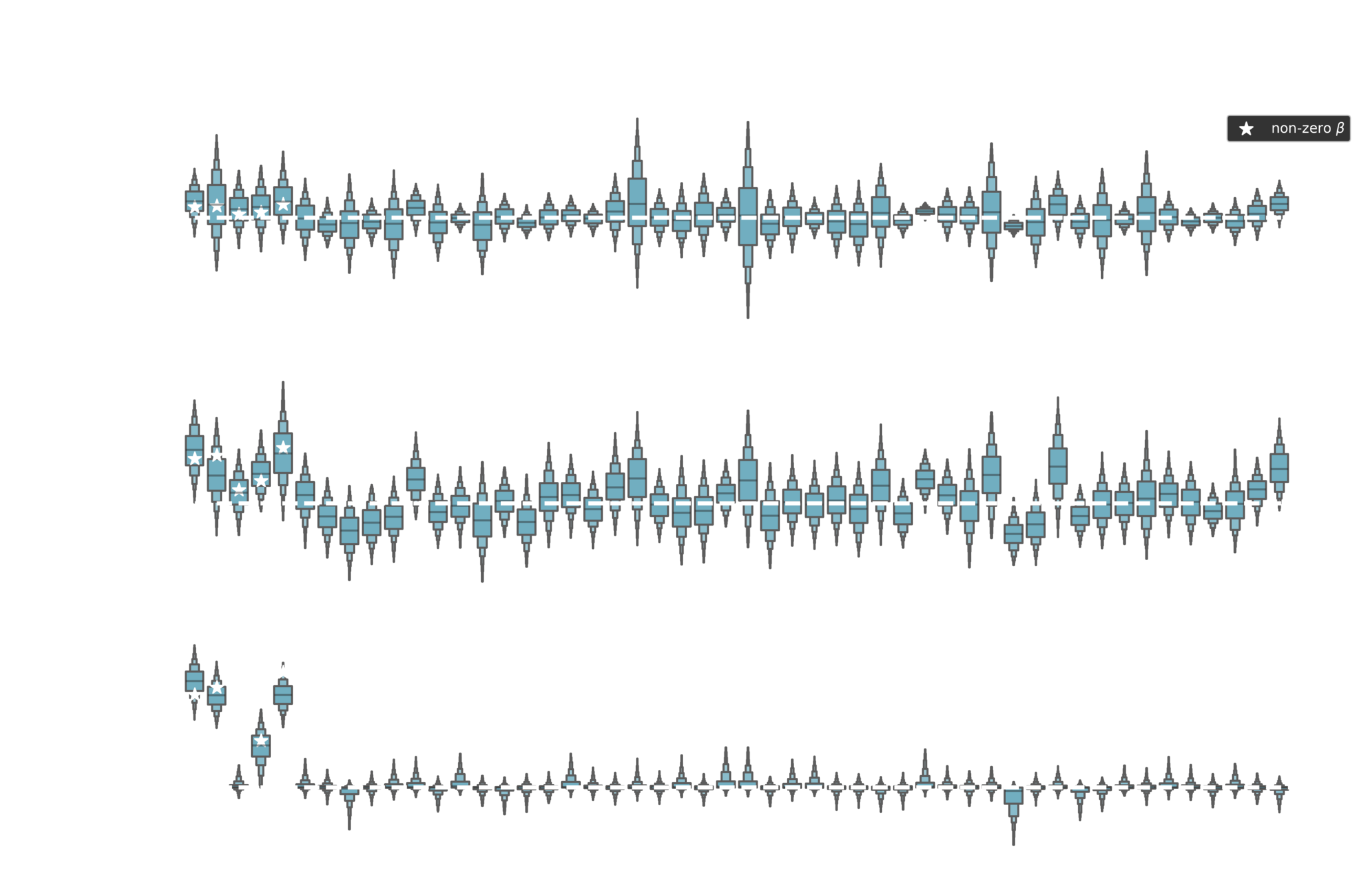
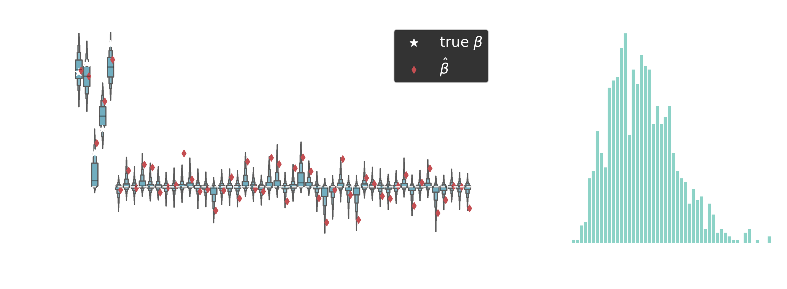
Non-zero coefficients

\tau \sim C^{+}(0, \tau_0^2)

Piironen, Juho, and Aki Vehtari. "Sparsity information and regularization in the horseshoe and other shrinkage priors." Electronic Journal of Statistics 11.2 (2017): 5018-5051.

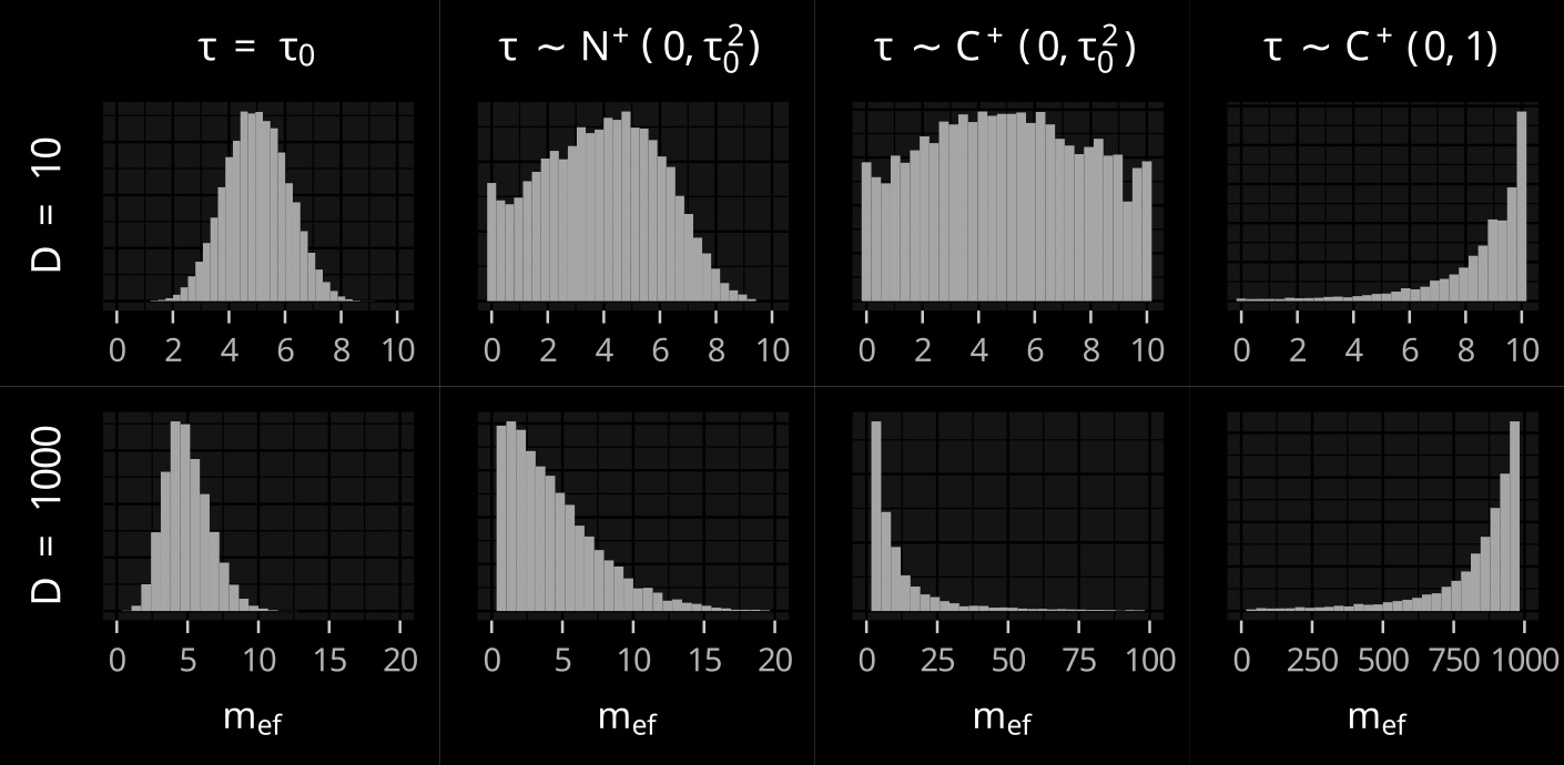
Effective number of

non-zero coefficients

m_{eff} = \sum_d (1 - \kappa_d)

Expected effective number

p_0 = E[m_{eff}|\tau] = \frac{\tau \sqrt{N}}{1 + \tau \sqrt{N}} D

\tau_0 = \frac{p_0}{D - p_0} \frac{1}{\sqrt{n}}

Effective number

Piironen, Juho, and Aki Vehtari. "Sparsity information and regularization in the horseshoe and other shrinkage priors." Electronic Journal of Statistics 11.2 (2017): 5018-5051.

N = 100,\:\: \sigma=1, p_0 = 5

Hierarchical shrinkage

\sigma^2 \sim \Gamma^{-1} \left(2, 2\right)\\ \tau_0 = \frac{p_0}{D - p_0} \frac{1}{\sqrt{n}} \\ \tau \sim C^+(0, \tau_0^2) \\ \lambda_d \sim C^+(0, 1) \\ \beta_d \sim \mathcal{N} \left(0, \sigma^2 \tau^2 \lambda^2_d \right) \\ \alpha \sim \mathcal{N}(0, 10)

Piironen, Juho, and Aki Vehtari. "Sparsity information and regularization in the horseshoe and other shrinkage priors." Electronic Journal of Statistics 11.2 (2017): 5018-5051.

prior constraint on the

number of nonzero coefficients

\( \rightarrow \)

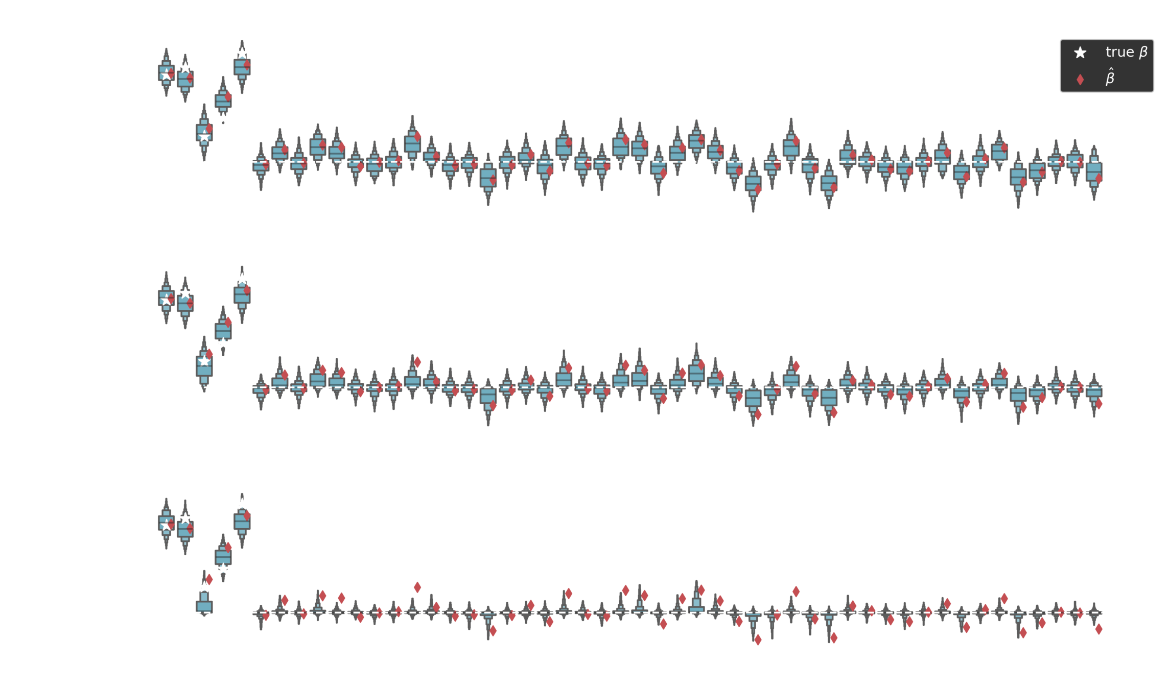
Posterior estimates

Outline

Bayesian regression
Hierarchical priors
Shrinkage priors
QR decomposition
Pairwise interactions

QR decomposition

\pmb{X}_k \sim \mathcal{N}_D \left( 0, \pmb{I}_D \right)

\pmb{X}^c_k \sim \mathcal{N}_D \left( 0, \pmb{\Sigma} \right)

\pmb{X}^c = \pmb{Q} \pmb{R}

Simulated data

D = 50, N = 200 \\ \alpha = 0, \quad X_k^c \sim \mathcal{N} \left(0, \pmb{\Sigma} \right) \\ \beta_{1}, \ldots, \beta_{S} > 0; \quad \beta_{d>S} = 0; \quad S=5 \\ \sigma = 1.

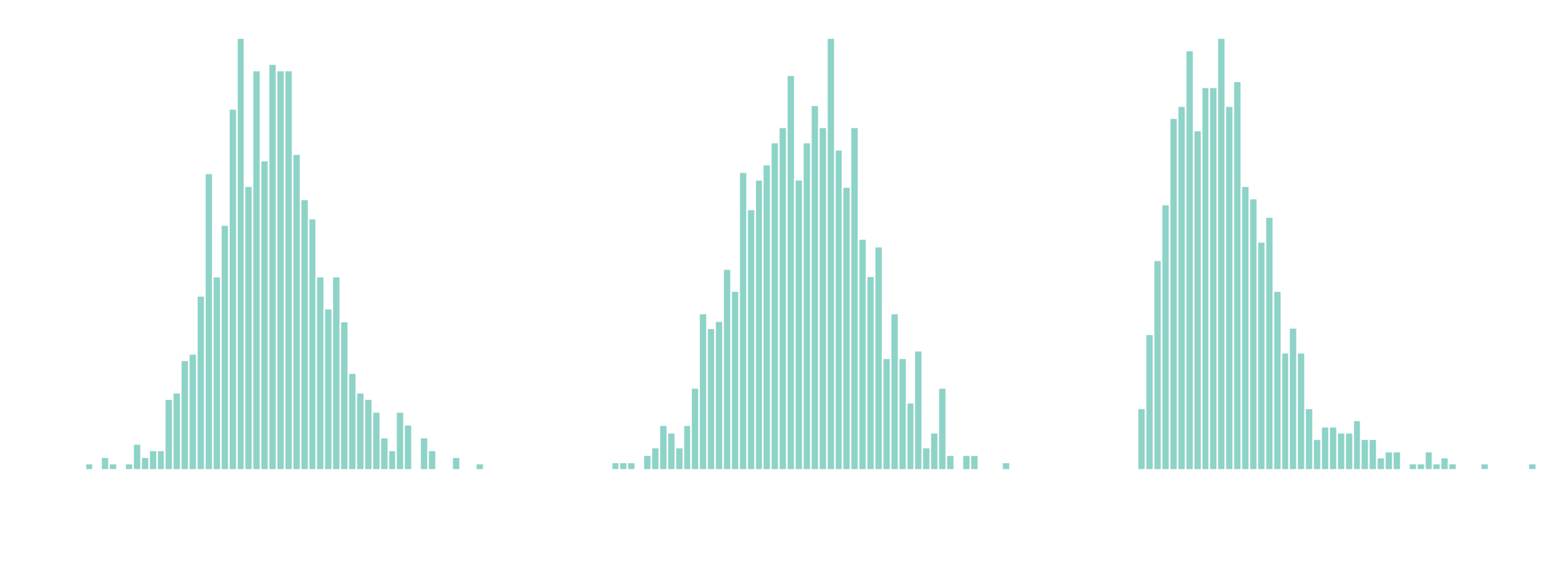
Posterior estimates

Outline

Bayesian regression
Hierarchical priors
Shrinkage priors
QR decomposition
Pairwise interactions

Pairwise Interactions

Agrawal, Raj, et al. "The kernel interaction trick: Fast bayesian discovery of pairwise interactions in high dimensions." International Conference on Machine Learning. PMLR, 2019.

\mu_k = \alpha + \sum_{i=1}^D \left[ \beta_i x_{i, k} + \sum_{j>i} \beta_{ij} x_{i, k} x_{j, k} \right] \\ y_k \sim p(y_k|\mu_k, \theta);\:\: \text{for } k \in \{1, \ldots, N\}

\mu_k = \alpha + \tilde{\pmb{X}}_k \cdot \tilde{\pmb{\beta}} \\

linear regression?

Structural prior

Agrawal, Raj, et al. "The kernel interaction trick: Fast bayesian discovery of pairwise interactions in high dimensions." International Conference on Machine Learning. PMLR, 2019.

\sigma^2 \sim \Gamma^{-1} \left(2, 2\right)\\ \alpha \sim \mathcal{N}(0, 10)

\tau_0 = \frac{p_0}{D - p_0} \frac{1}{\sqrt{n}} \\ \tau_1 \sim C^+(0, \tau_0^2) \\ \lambda_i \sim C^+(0, 1) \\ \beta_i \sim \mathcal{N} \left(0, \sigma^2 \tau_1^2 \lambda^2_i \right) \\

\tau_2 \sim C^+(0, \tau_1^2) \\ \beta_{ij} \sim \mathcal{N} \left(0, \sigma^2 \tau_2^2 \lambda^2_i \lambda^2_j \right) \\

The kernel interaction trick

Agrawal et al. demonstrates how one can express the linear regression problem (with pairwise interactions) as a Gaussian process model using specific kernel structure.

The Gaussian process models have better scaling with D, but further approximations are needed for larger N.

To me it is unclear if the approach can be applied to nonlinear GLMs.

Discussion

Hierarchical shrinkage priors are essential for separating signal from noise in the presence of correlations.

Structural shrinkage priors help separate linear

and pairwise contributions to the "responses".

https://github.com/dimarkov/pybefit

Generalises to Logistic regression, Poisson regression, etc.