HOW DO
MACHINES
LEARN I

https://slides.com/djjr/ryanct-how-do-machines-see

EN.501.152.FA25

Ryan: FYS Computational Reasoning Fall 2025

Lecture content licensed under a Creative Commons Attribution-NonCommercial-ShareAlike 4.0 International License.

Part 4 LLMs

LEARN III: Reinforcement Learning

LEARN II: Deep Learning

LEARN I: Supervised Learning and Classification

2019 Slide Deck

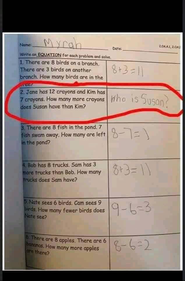
OUTTAKES

mea culpa

*


	-1

		+1	-1	-1
				-1
	-1

ISCHOOL VISUAL IDENTITY

#002554

#fed141

#007396

#382F2D

#3eb1c8

#f9423a

#C8102E

INTRO

max pooling

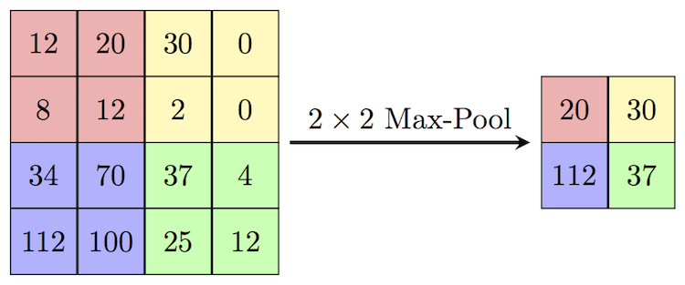
Question from last class...

max pool = downsample by taking largest value from each pool (one might also average pool)

Pooling and Convolutions are two families of filters. There are others...

Normalization filters adjust values in a region to have more stable distributions.

Attention or adaptive filters learn which spatial locations to emphasize.

Supervised Learning

Regression

Classification

Great Quick Course

Google Dev Intro to Machine Learning

Google Dev Crash Course: Linear regression

Google Dev Crash Course: Logistic regression

Google Dev Crash Course: Classification

Regression: predict Y from X

Logistic Regression: predict P(YES/NO) from X

and

What is KERAS? Keras is a high-level, open-source deep learning API written in Python

Keras is a high-level abstraction for building neural networks, hiding the complexities of lower-level frameworks like TensorFlown or PyTorch.

Make a copy of this notebook in your google drive.

Preliminaries
Install required libraries

Load dependencies
Load the dataset & Update the dataframe & Read dataset

Dataset Exploration
View dataset statistics
Generate a correlation matrix
Visualize relationships in dataset

Part 3 - Train Model

Experiment with Model

https://tinyurl.com/y59r3h4c

Classification

Make a copy of this notebook in your google drive.

Preliminaries
Load libraries & dependencies & dataset
Dataset Exploration

Visualize

Normalize
Prepare experiments

Train Simple Model

Evaluate

Train Full Model

Evaluate

Compare

Binary Classification

https://tinyurl.com/5hd3nhyu

(Unsupervised Learning)

HOW DO
MACHINES
LEARN II (DL)

https://slides.com/djjr/ryanct-how-do-machines-see

EN.501.152.FA25

Ryan: FYS Computational Reasoning Fall 2025

Lecture content licensed under a Creative Commons Attribution-NonCommercial-ShareAlike 4.0 International License.

Deep Learning
(DL)

https://tinyurl.com/ryan-ct25-dl-demo

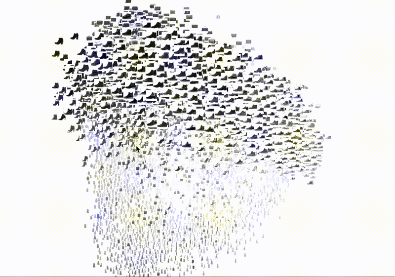
MNIST (Modified National Institute of Standards and Technology) Fashion Dataset

model = tf.keras.Sequential([
    tf.keras.layers.Flatten(input_shape=(28, 28)), # convert 28x28 matrix into 784x1 input layer
    tf.keras.layers.Dense(128, activation='relu'), # 1st hidden layer has 128 nodes
    tf.keras.layers.Dense(10)                      # 2nd hidden layer has 10 nodes
])

tf.keras.layers.Flatten(input_shape=(28, 28))

tf.keras.layers.Dense(128, activation='relu')

tf.keras.layers.Dense(10)

LOGITS

STEP 1 Set up the layers

Other Model Architectures

More or fewer layers

model = tf.keras.Sequential([
    tf.keras.Input(shape=(28, 28)),
    tf.keras.layers.Flatten(),
    tf.keras.layers.Dense(256, activation='relu'),
    tf.keras.layers.Dense(128, activation='relu'),
    tf.keras.layers.Dense(10)
])

Different Activations

tf.keras.layers.Dense(128, activation='tanh')
tf.keras.layers.Dense(128, activation='sigmoid')
tf.keras.layers.Dense(128, activation='leaky_relu')

Regularization and Normalization Layers

# DROPOUT - Used to prevent overfitting and improve
# training stability.

tf.keras.layers.Dropout(0.5)


# BATCH NORMALIZATION Normalizes layer outputs 
# to stabilize learning.

tf.keras.layers.BatchNormalization()

Convolutions and Recurrent Networks

# Convolutional Layers (CNNs): Fashion-MNIST is 
# grayscale/simple, but CNNs dramatically improve accuracy.

model = tf.keras.Sequential([
    tf.keras.Input(shape=(28, 28, 1)),    # need channel dimension
    tf.keras.layers.Conv2D(32, (3, 3), activation='relu'),
    tf.keras.layers.MaxPooling2D((2, 2)),
    tf.keras.layers.Conv2D(64, (3, 3), activation='relu'),
    tf.keras.layers.MaxPooling2D((2, 2)),
    tf.keras.layers.Flatten(),
    tf.keras.layers.Dense(64, activation='relu'),
    tf.keras.layers.Dense(10)
])


# Recurrent Layers (RNNs, LSTMs, GRUs) for 
# sequence data (less typical for images

model = tf.keras.Sequential([
    tf.keras.Input(shape=(28, 28)),  # interpret each row as a timestep
    tf.keras.layers.SimpleRNN(64),
    tf.keras.layers.Dense(10)
])

# or

tf.keras.layers.LSTM(64)
tf.keras.layers.GRU(64)

adam: adaptive optimization algorithm that adjusts learning rates for each parameter

Others you'll hear of are Stochastic Gradient Descent (SGD) - simplest and oldest or Adagrad (adjusts learning rates based on how frequently parameters get updated)

STEP 2 COMPILE THE MODEL

Specify the optimizer (how the model weights are updated), the loss function (how to calculate the error), and metrics (how we will monitor the training and testing, for example, accuracy)

model.compile(optimizer='adam',
              loss=tf.keras.losses.SparseCategoricalCrossentropy(from_logits=True),
              metrics=['accuracy'])

The TensorFlow Keras API

submodule that contains loss functions

Which loss function (there are lots of choices)

Sparse: labels are integers not one-hot vectors

Categorical: multiclass classification

Crossentropy: computes difference between two distributions

what algorithm to adjust weights with

“my model outputs raw scores — please apply softmax inside the loss function.”

track and report fraction of predictions that match labels

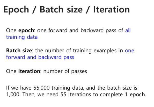
STEP 3 Train the model

model.fit(train_images, train_labels, epochs=10)

fit(x, y, batch_size=NONE, epochs)

If batch_size is not specified it defaults to 32. The model:

computes their predictions for 32 images,
calculates average,
adjusts weights,
repeats for the next 32 images.

STEP 4 Evaluate accuracy

test_loss, test_acc = model.evaluate(test_images,  test_labels, verbose=2)

print('\nTest accuracy:', test_acc)

evaluate(x=None, y=None, batch_size=None, verbose='auto'

Returns the loss value & metrics values for the model in test mode.

0 = silent, 1 = progress bar, 2 = single line

STEP 5 Make Probability Predictions

probability_model = tf.keras.Sequential([model,                        
                                         tf.keras.layers.Softmax()])   

predictions = probability_model.predict(test_images)

model = keras.Sequential( layers=None )

returns Model object

the 3 layer model we already built

the layer we want to add on

softmax converts logits
to probabilities

groups a linear stack of layers,

σ(z) _i =\frac{e^ {z_ i}}{ ∑ _{j=1} ^K e^ {z_ j} }

run this model on this data

LOGITS

softmax

def plot_image(i, predictions_array, true_label, img):
  true_label, img = true_label[i], img[i]
  plt.grid(False)
  plt.xticks([])
  plt.yticks([])

  plt.imshow(img, cmap=plt.cm.binary)

  predicted_label = np.argmax(predictions_array)
  if predicted_label == true_label:
    color = 'blue'
  else:
    color = 'red'

  plt.xlabel("{} {:2.0f}% ({})".format("P:" + class_names[predicted_label],
                                100*np.max(predictions_array),
                                "L:" + class_names[true_label]),
                                color=color)

def plot_value_array(i, predictions_array, true_label):
  true_label = true_label[i]
  plt.grid(False)
  plt.xticks(range(10))
  plt.yticks([])
  thisplot = plt.bar(range(10), predictions_array, color="#777777")
  plt.ylim([0, 1])
  predicted_label = np.argmax(predictions_array)

  thisplot[predicted_label].set_color('red')
  thisplot[true_label].set_color('blue')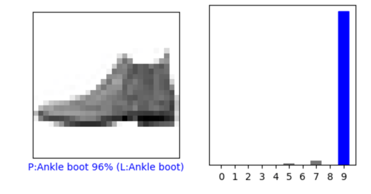

https://tinyurl.com/CTFYS25-fastai-demo

HOW DO
MACHINES
LEARN III (RL)

https://slides.com/djjr/ryanct-how-do-machines-see

EN.501.152.FA25

Ryan: FYS Computational Reasoning Fall 2025

Lecture content licensed under a Creative Commons Attribution-NonCommercial-ShareAlike 4.0 International License.

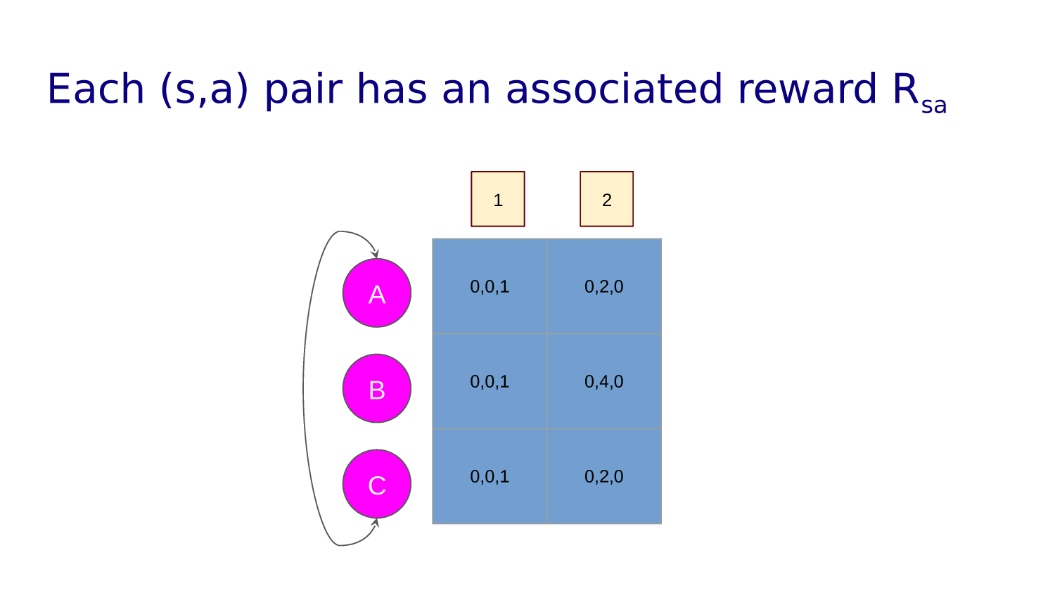
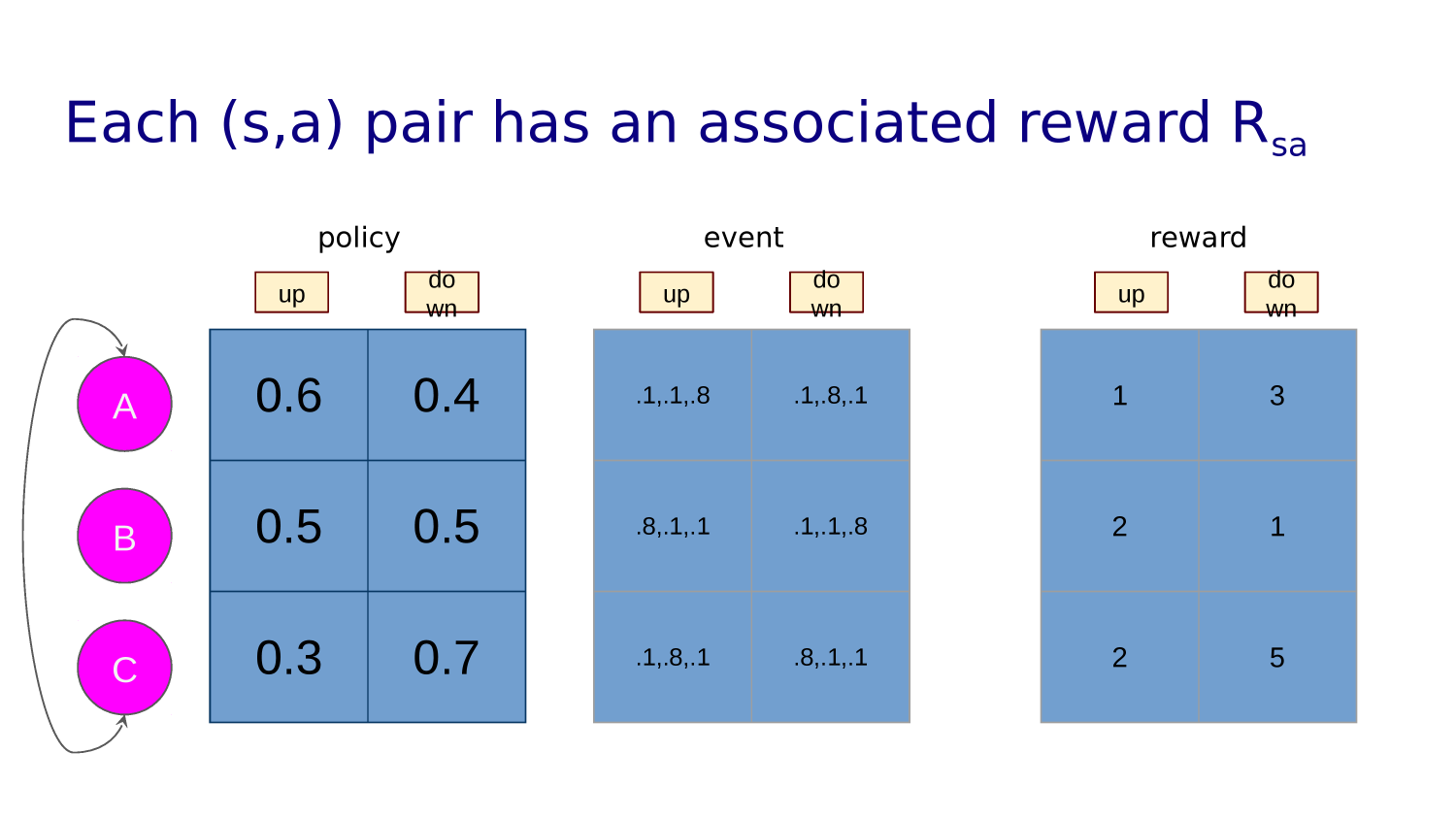
Reinforcement Learning (RL)

How does a machine learn to play a video game?

$$

start

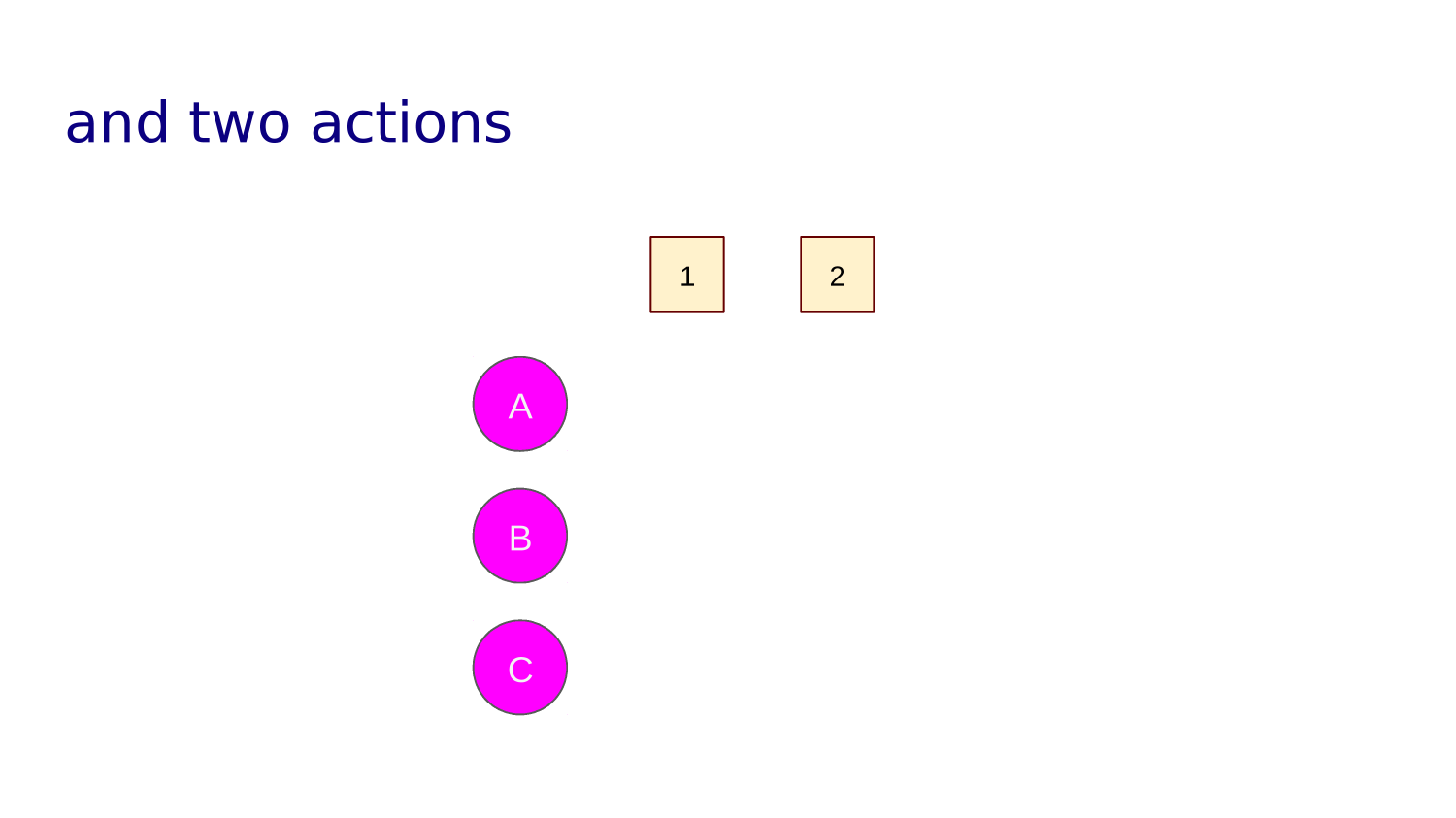
actions
UP, DOWN, LEFT, RIGHT

GRIDWORLD

REWARDS

PUNISHMENTS

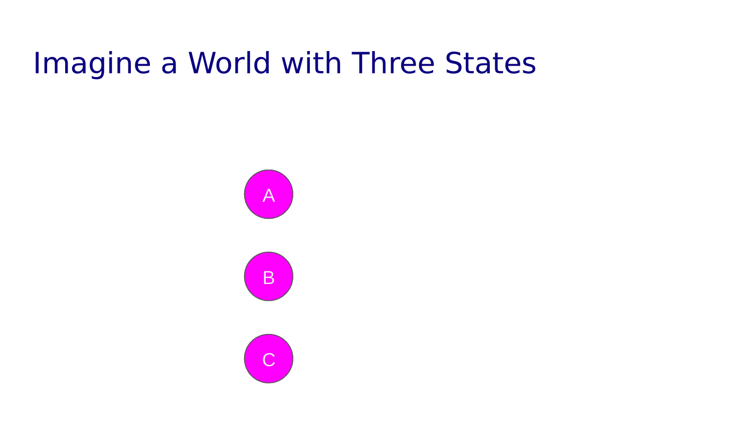
Each square is a "state"

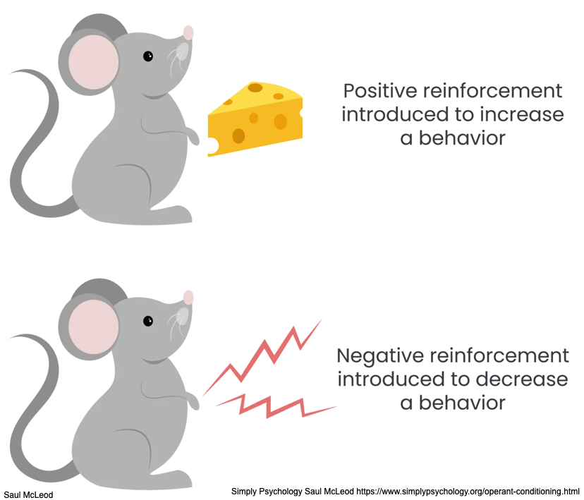
Animal Reinforcement Learning

0	1	2	3	4	5	6	7	8	9
10	11	12	13	14	15	16	17	18	19
20	21	22	23	24	25	26	27	28	29
30	31	32	33	34	35	36	37	38	39
40	41	42	43	44	45	46	47	48	49
50	51	52	53	54	55	56	57	58	59
60	61	62	63	64	65	66	67	68	69
70	71	72	73	74	75	76	77	78	79
80	81	82	83	84	85	86	87	88	89
90	91	92	93	94	95	96	97	98	99

GRIDWORLD

\text{100 states, } s_i \in \mathbf{S}

\text{4 actions, } a_i \in \mathbf{A}=\{\text{U}, \text{R}, \text{D}, \text{L}\}

\text{Transition function, } T: \mathbf{S} \times \mathbf{A} \rightarrow \mathbf{S}

FROM	U	R	D	L
0	0	1	10	0
1	1	2	11	0
2	2	3	12	1
3	3	4	13	2
4	4	5	14	3
...
10	0	11	20	10
11	1	12	21	10

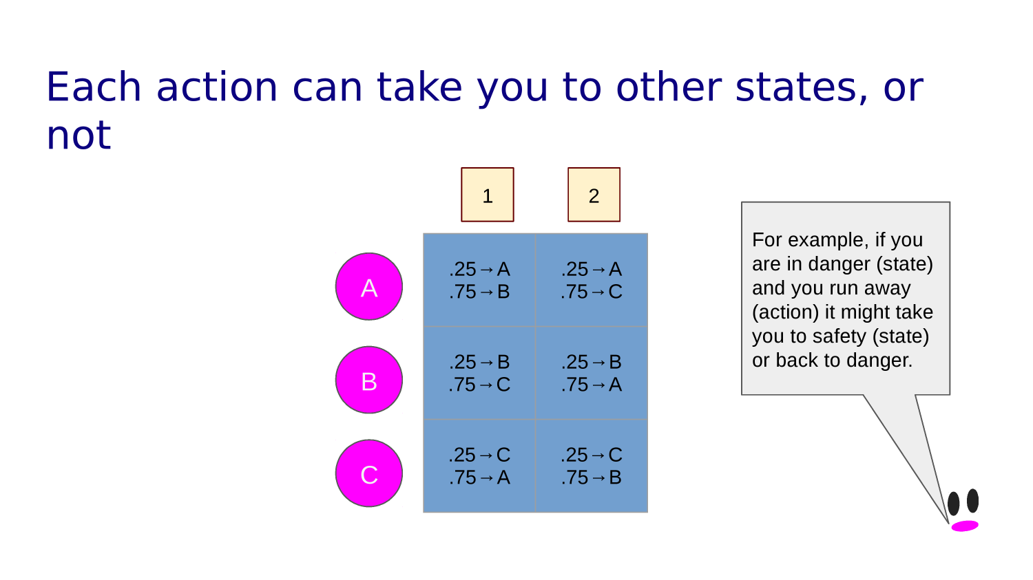
Transition function tells you what state each action leads to from any given state.

0	1	2	3	4
10	11	12
20

IMPENETRABLE BARRIER

GridWorlds Have Walls

In a grid world, some cells may be off limits.

If our action takes us into a wall or off the grid we just bounce back into the state we came from.

FROM	U	R	D	L
0	0	1	10	0
1	1	2	11	0
2	2	3	12	1
3	3	4	13	2
4	4	5	14	3
...
10	0	11	20	10
11	1	12	11	10


	-1
	-1
-1

	+1	-1
			-1
-1

IMPENETRABLE BARRIER

GridWorld

GOAL

Some states yield rewards or punishments.

Awards are earned when the agent lands in such a state.

A GOAL state can be the end of an agent's "turn."






					+1

IMPENETRABLE BARRIER

GridWorld

Imagine a grid world with a single rewarding state.

We can represent the policy for a given state with an arrow diagram. For example, this:

would mean our policy in this state is go up 25% of the time, down 25% of the time and right 50% of the time.






					+1

IMPENETRABLE BARRIER

GridWorld

GOAL

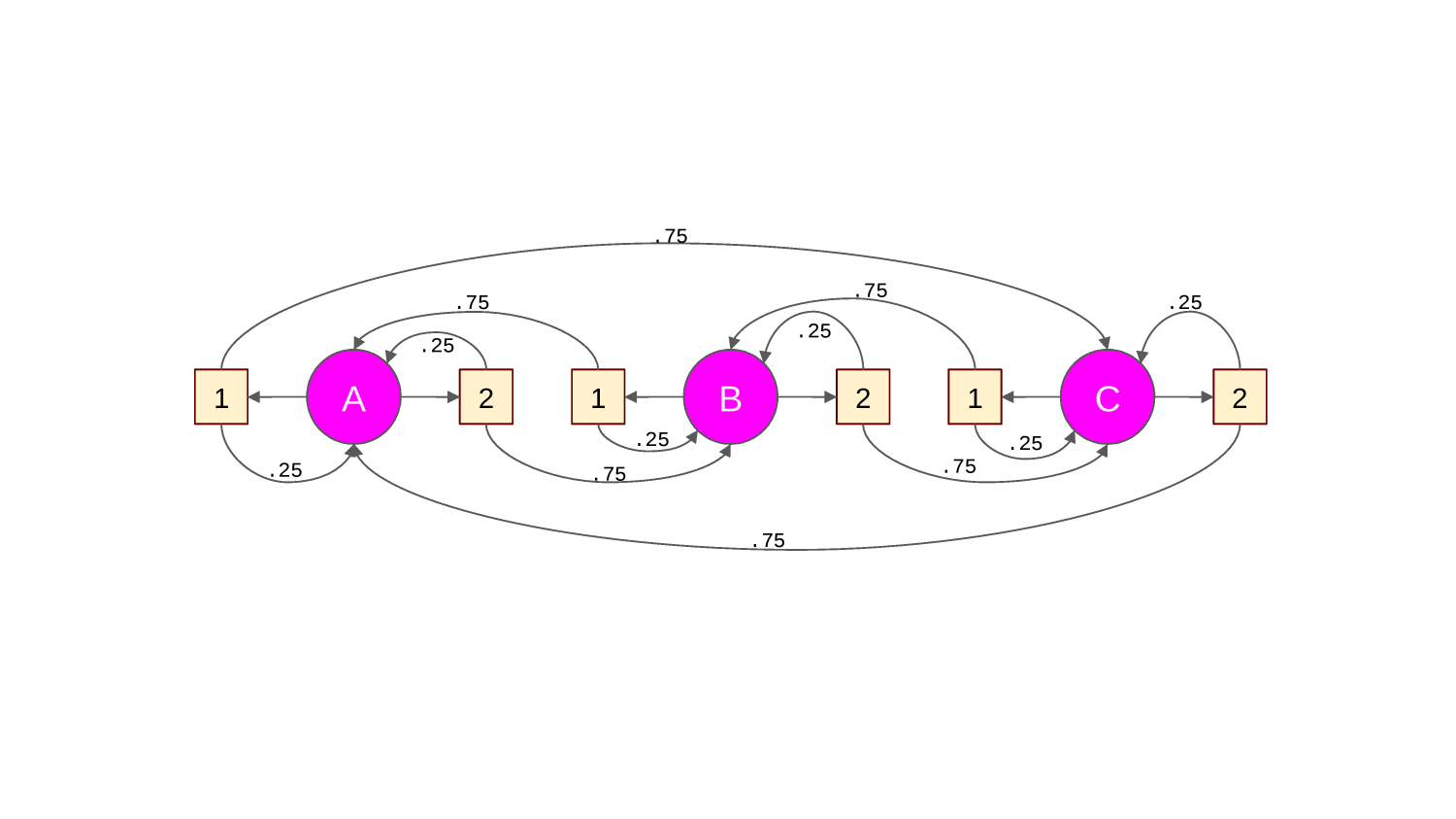
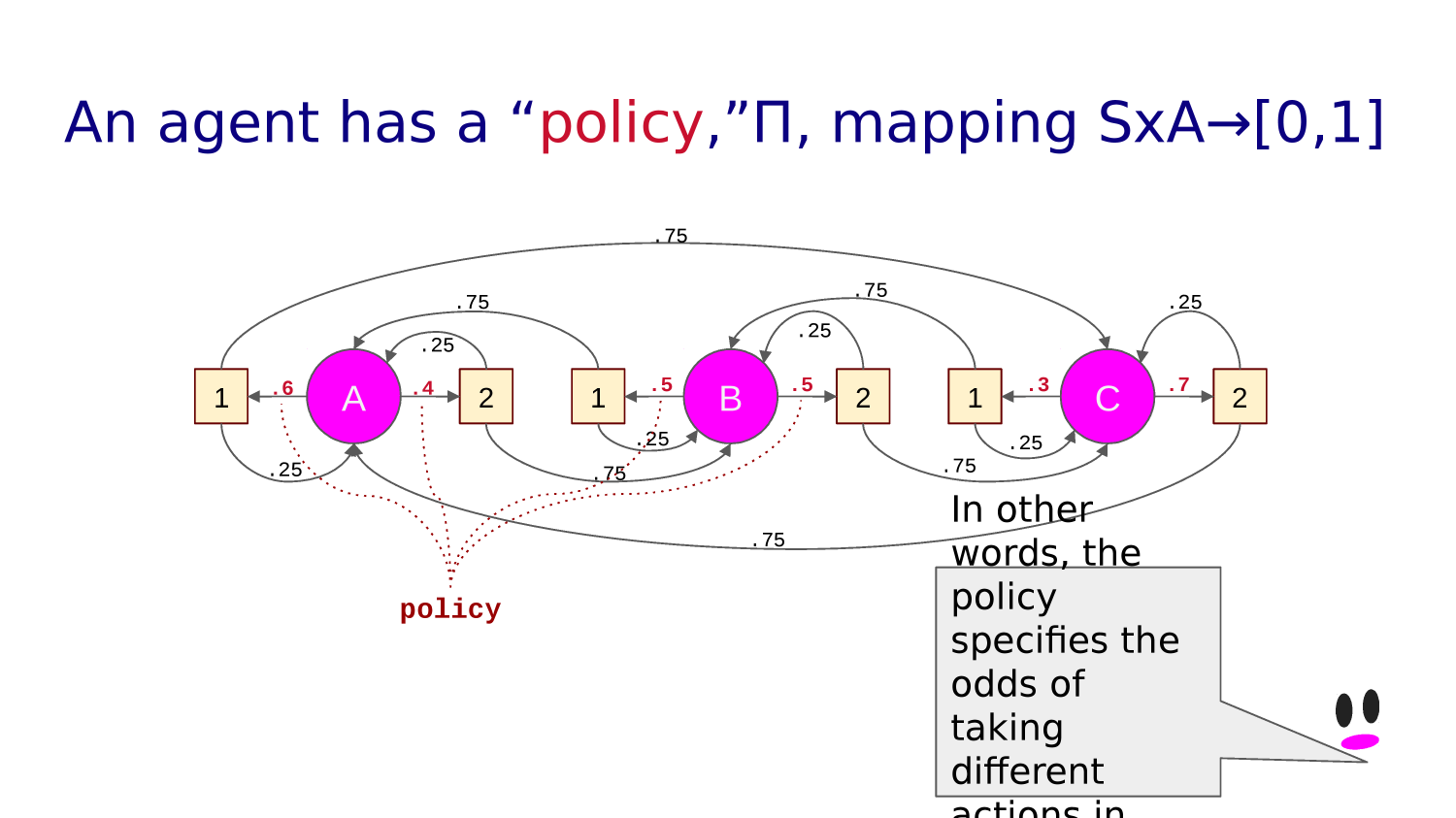
For every state, an agent has a "POLICY": what action it will take with what probability.

\text{Policy, } \pi : \mathbf{S} \rightarrow \mathbf{A}

We can represent the policy for a given state with an arrow diagram. For example, this:

would mean our policy in this state is go up 25% of the time, down 25% of the time and right 50% of the time.

Training an RL agent means learning a policy that allows it to maximize the reward it collects.

It learns the optimal policy by trial and error, living the same day over and over again.

STOP+THINK: What is Phil doing as he lives the day over and over again?






					+1

START

IMPENETRABLE BARRIER

GridWorld

GOAL

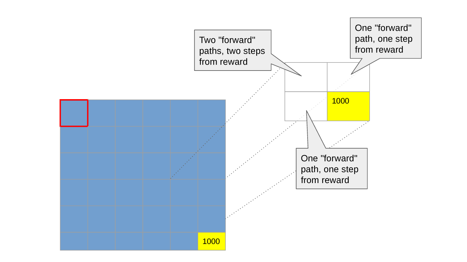
In the start state we have two action to choose from: right or down.

All paths lead eventually to the reward (that's where they stop), but some faster than others.

Moving right takes us to state 1, moving down takes us to state 10.

How should we compare them? Which one is better? What should our policy be in state 0?

Both are the "first steps of the rest of your life."

Both are the first step on an infinity of possible paths.

If we imagine each step takes a little bit of energy, we would expect that the net reward will be less for shorter paths.

So, maybe we can compare state 1 and state 10 by taking the average of the net reward earned by all of the paths that start with one or the other?

START

IMPENETRABLE BARRIER

GridWorld

100
GOAL

To make the math easy, let's assume that reward at the goal is 100.

And so on.

And let's formalize that each step takes energy by saying that each step costs 10% of the reward you get in the next state. We say that we have a 90% discount rate, "gamma."

So we can imagine an algorithm that begins: start from the goal state and identify any state that leads to it in one step.

Assign a value to those states that is the discount rate times the reward of the goal state.

So, one step away that 100 is worth 0.9x100=90.

Now, repeat this process for any state that leads to one of these states in one step.

This is not quite exactly right though because we want to base this on what the agent would actually do in each state.

And two steps away it is 0.9²x100=81.

\text{Discount rate } \gamma = 0.9

Life can only be understood backwards; but it must be lived forwards.
― Søren Kierkegaard (1813-1855)

Kierkegaard was right...

...but the math of that is challenging

START

IMPENETRABLE BARRIER

GridWorld

100
GOAL

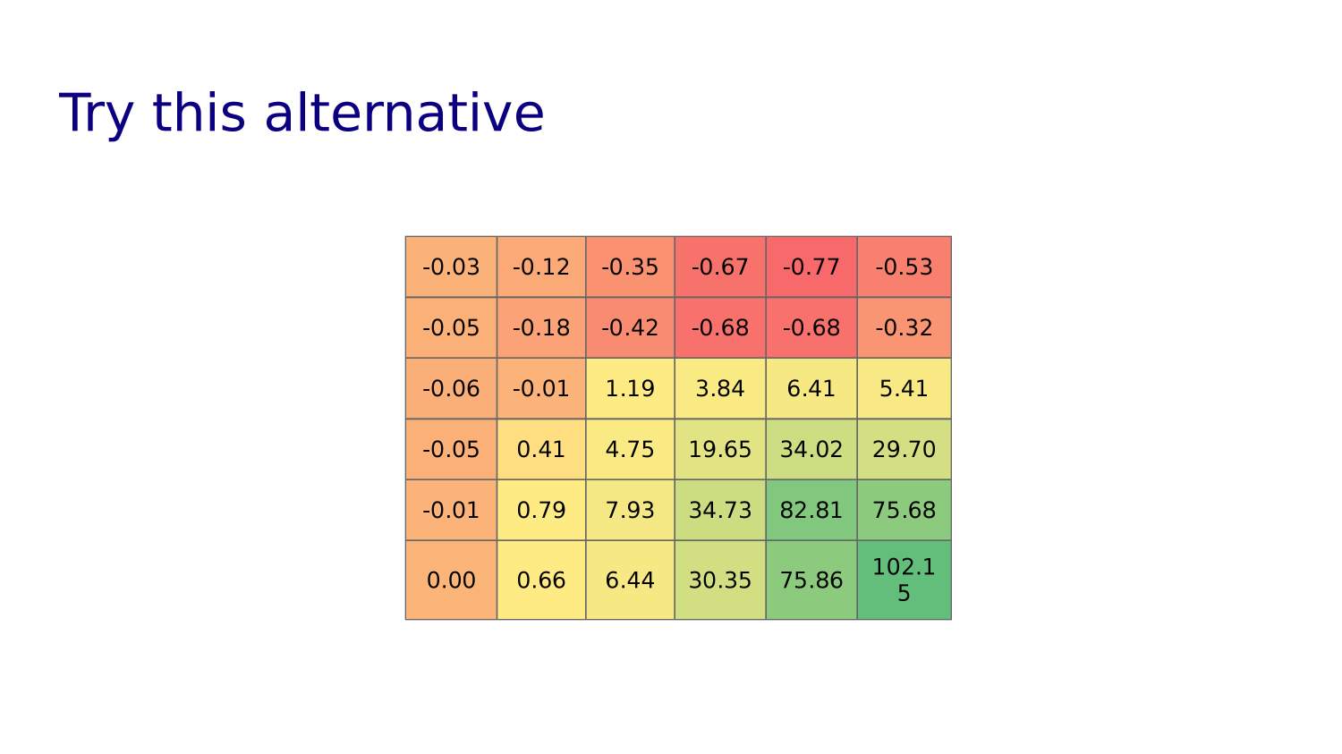
If we were to continue that process we can imagine arriving at a "heat map" picture of the "value" of each state that looked like this.

Again, it's not quite right because we haven't taken into account how the agent would move (that is, what its POLICY is).

If we represent the relative probability of each direction we can choose by the size of an arrow, then equally likely in four directions would look like this

Before it has learned anything about its environment, we can assume the policy is to randomly choose from among the valid moves in any given state.

And equally likely in three directions would look like this

START

IMPENETRABLE BARRIER

GridWorld

100
GOAL

So here's what our initial random policy might look like.

	9	8	7	6	5
15					4
14					3
13					2
12	11				1
	10
	9	8			1
		7			2
		6	5	4	3

+100
GOAL

Each state can be characterized by how close it is to the reward. Here we have worked backward from the goal (in state 55 - row 6 column 6) applying a discount factor of 0.9.*

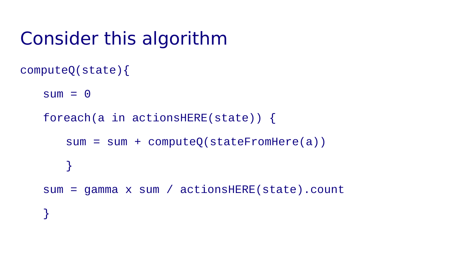
By "close" we mean something like "what is the average reward associated with all the paths that start here (conditioned by the likelihood that I choose them according to my policy)?".

Does that sound a little recursive? It is!

*truth in advertising: these numbers are a little fudgy but the spirit is right. Take a look at the upper left hand corner.

STOP+THINK: Why might these two states have different values?


	-1
	-1
-1

	+1	-1
			-1
-1

START

IMPENETRABLE BARRIER

GridWorld Summary

GOAL

In a grid world, the cells in the grids are states.

An agent can move left, up, right, and down.

Sometimes an action is blocked by a wall or the edge of the world.

A "transition function" maps state action pairs to the next state. For example:

T(0,L)=0, T(0,U)=0,
T(0,R)=1, T(0,D)=10

A trained agent has a "policy" - what action it will take in any given state.

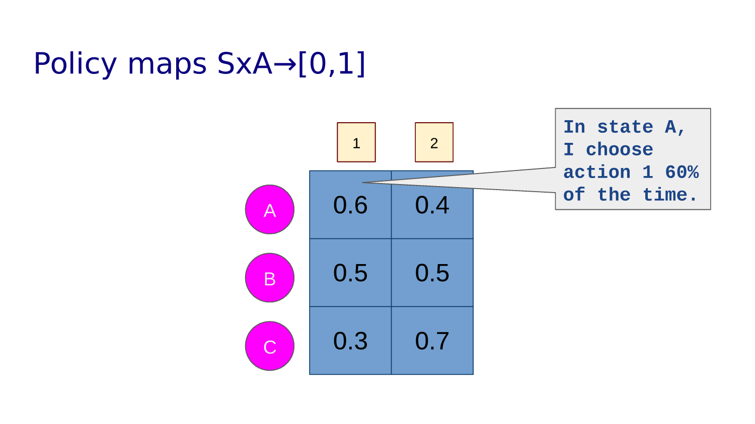
A policy maps state, action pairs to a probability. For example:

P(0,L)=0.3, P(0,U)=0.2, P(0,R)=0.1, P(0,D)=0.4

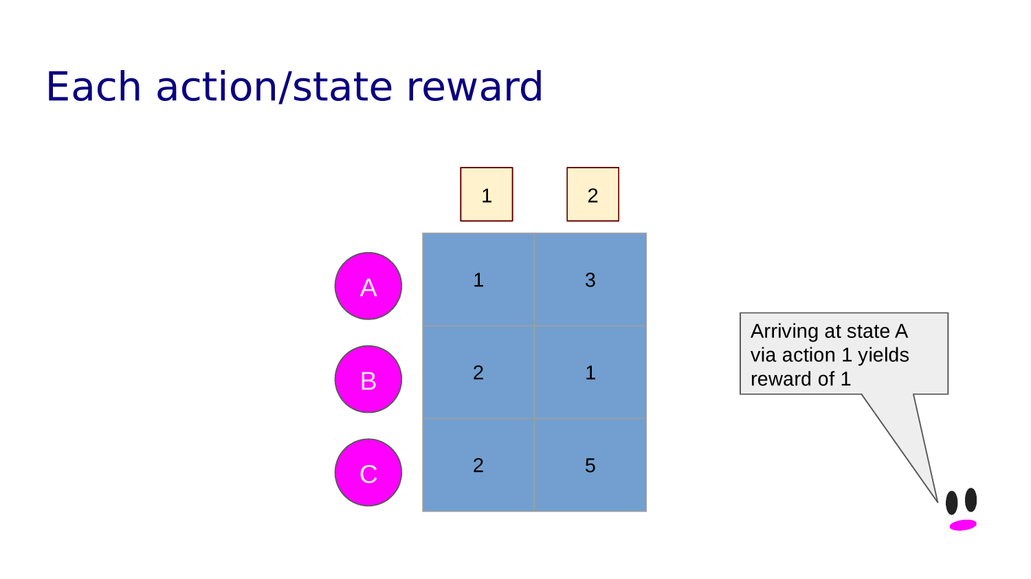
Some states yield rewards or punishments.

Awards are discounted over time. An agent wants a policy that maximize its total reward.

state 0

https://cs.stanford.edu/people/karpathy/reinforcejs/gridworld_dp.html

\begin{align*} V^\pi(s) & = E_\pi \{ r_t + \gamma r_{t+1} + \gamma^2 r_{t+2} + \ldots \mid s_t = s \} \\ & = E_\pi \{ r_t + \gamma V^\pi(s_{t+1}) \mid s_t = s \} \\ & = \sum_a \pi(s,a) \sum_{s'} \mathcal{P}_{ss'}^a \left[ \mathcal{R}_{ss'}^a + \gamma V(s') \right] \end{align*}

https://tinyurl.com/5n8n2crd

10x10 GridWorld

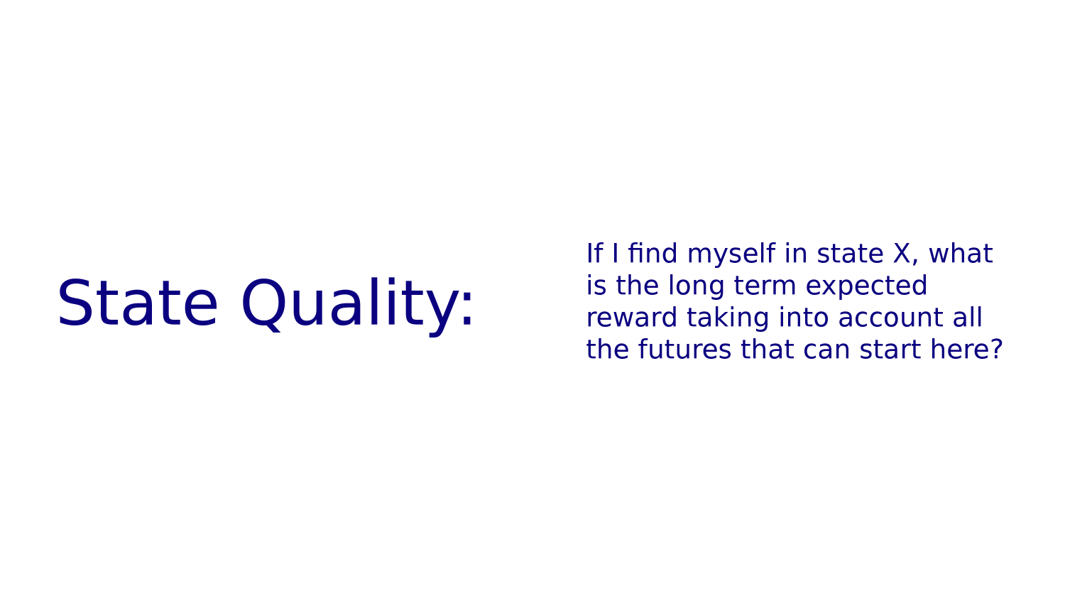
state "Quality" estimate

policy in this state

reward in this state

walls

goal state

+100
GOAL

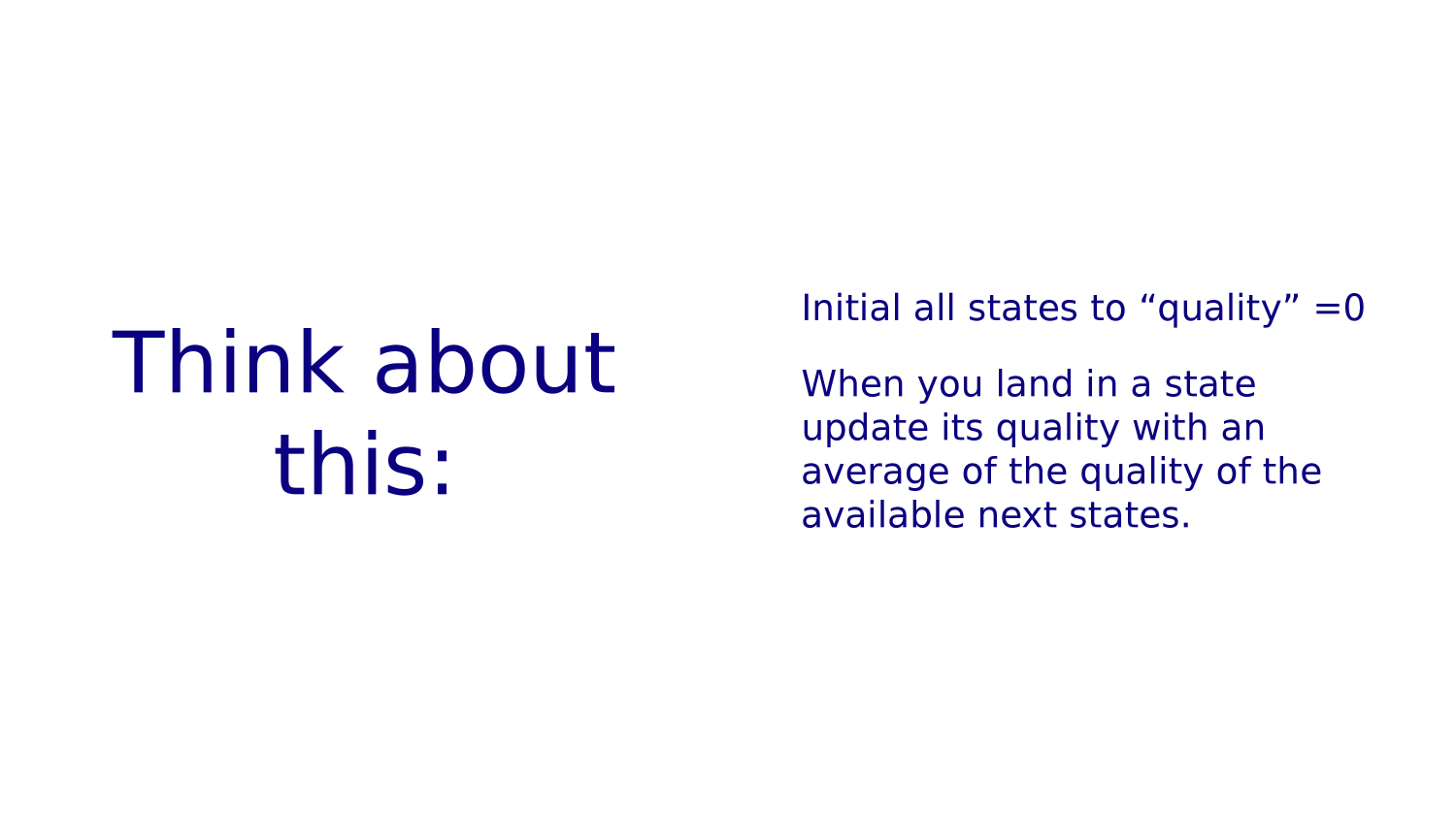
Each action is the first step in an "infinite" number of futures.

The "quality" (Q) of the cell into which that first step takes us is the average of the rewards of all the futures that begin with that step.

0	1	2	3	4	5	6	7	8	9
10	11	12	13	14	15	16

r,c

START

+100
GOAL

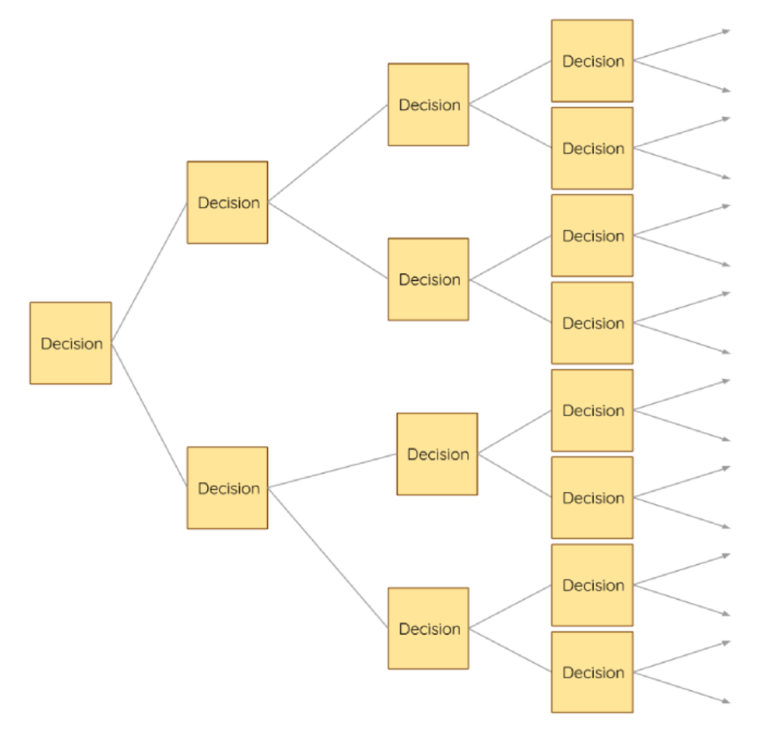
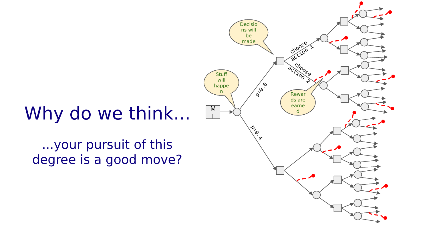
Another way to look at it is like a big decision tree (only selected nodes are shown). The policy gives the

START

	9	8	7	6	5
15					4
14					3
13					2
12	11				1
	10
	9	8			1
		7			2
		6	5	4	3

+100
GOAL

r,c

START

Some "lives" take longer to get to the goal. If all of the reward comes upon reaching the goal, shorter paths are more valuable because deferred rewards are "discounted."

Helpful Requisites

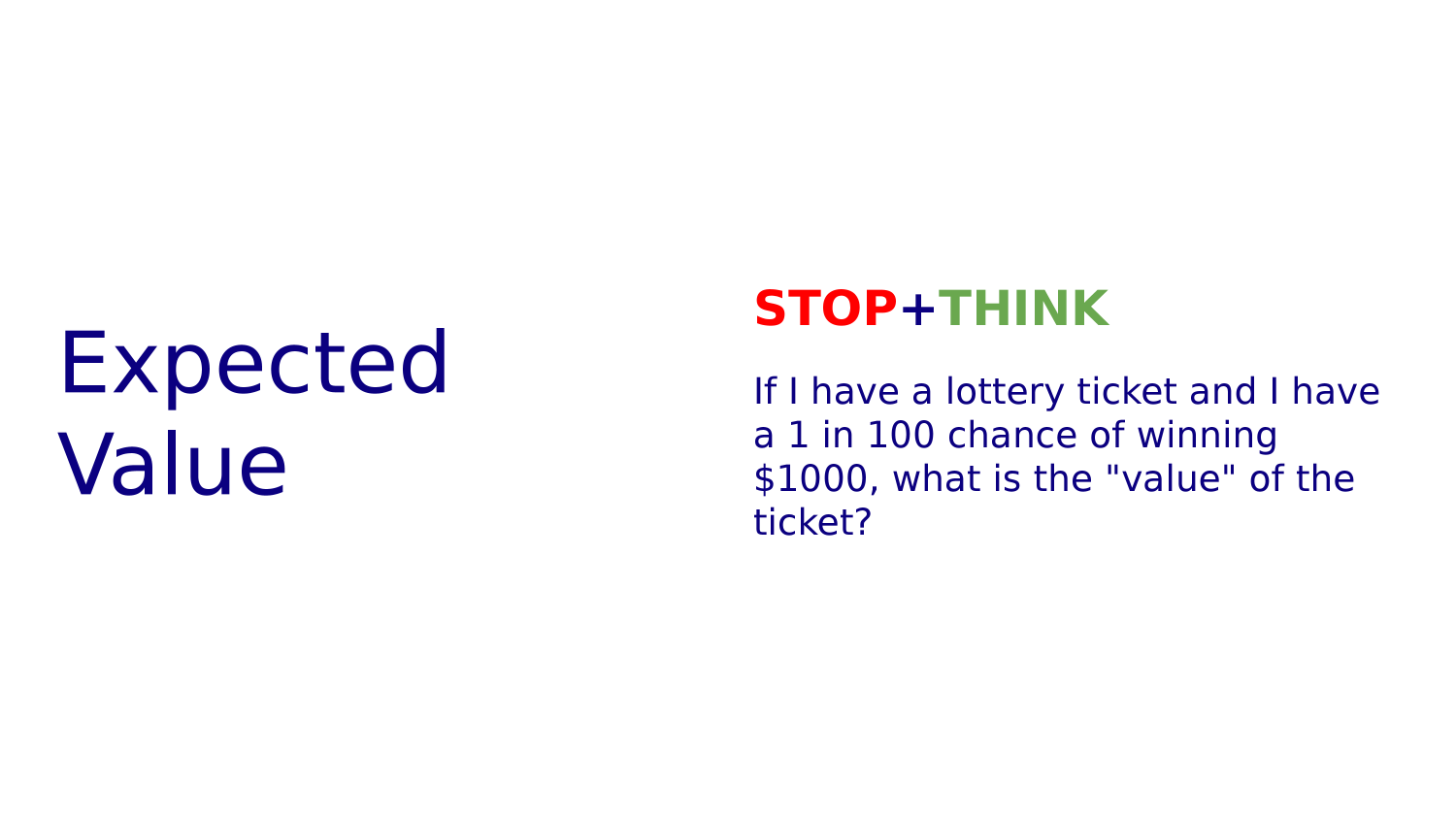
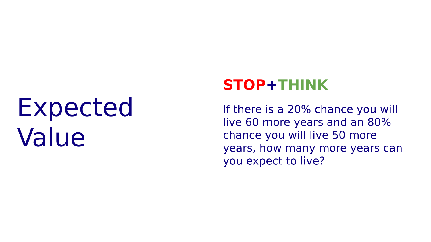
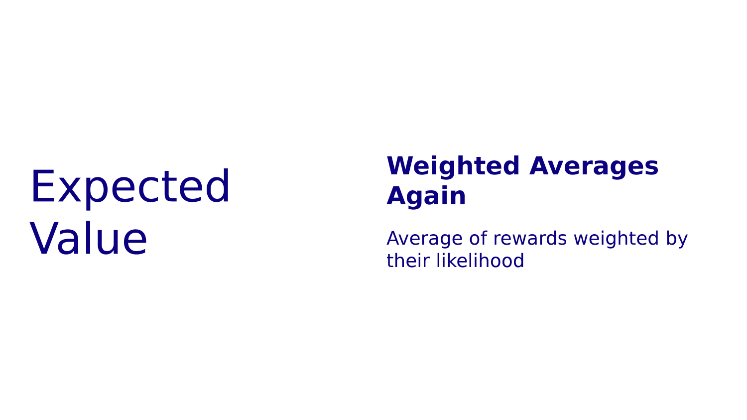
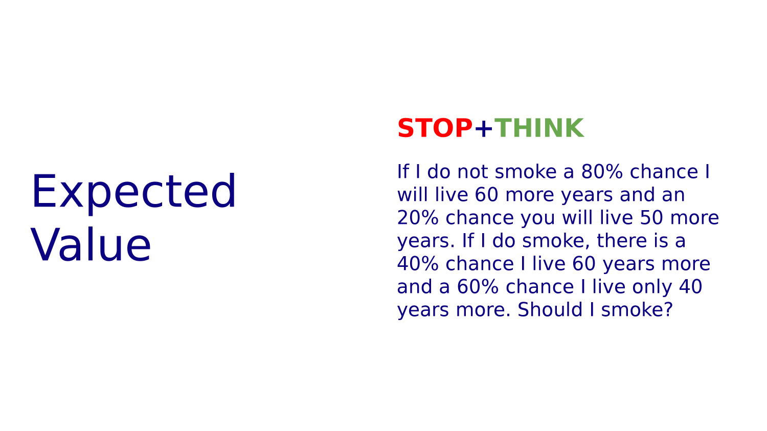
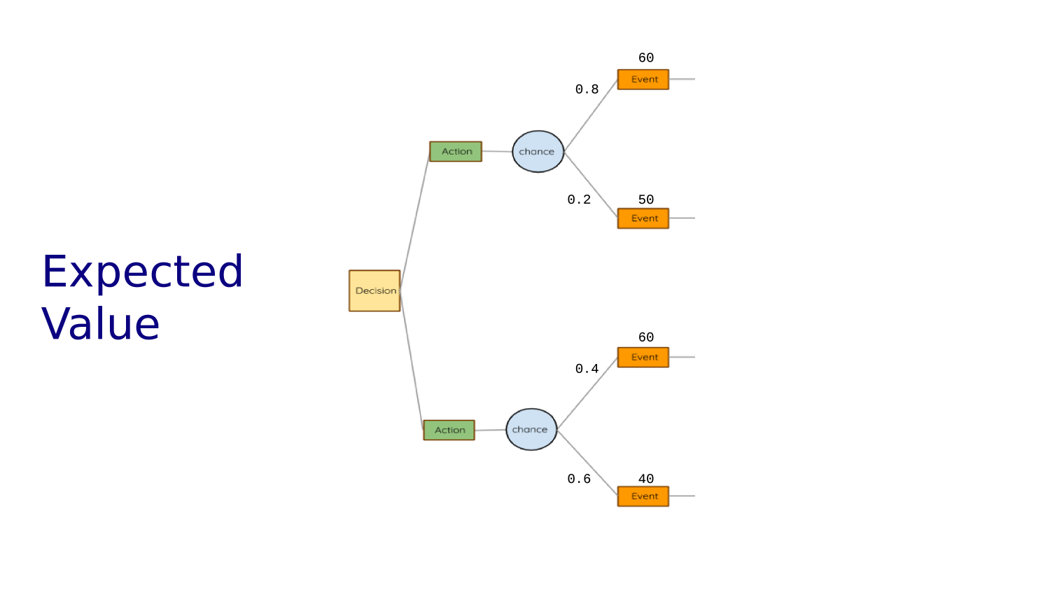
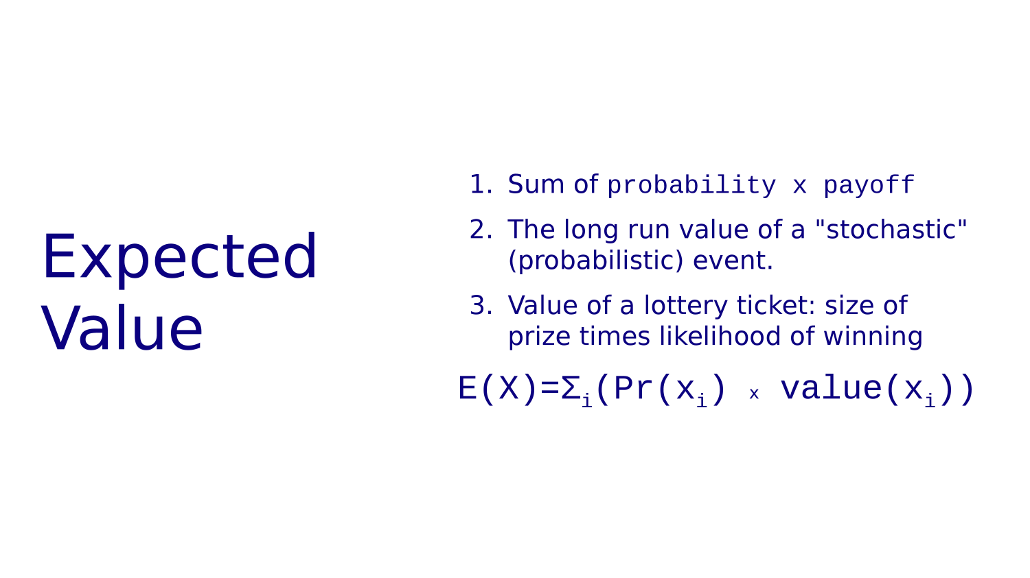
Expected Value

Discounting

RL Primer Worksheet

\text{Expected Value }=\sum_i X_i P(X_i)

If a coin toss game features a fair coin and $2 for heads and -$1 for tails what is the expected value of a single toss?

Suppose the coin is not fair; it comes up tails 69% of the time?

If a dice toss game features tossing a single fair die and the payoffs are plus face value for even numbers and minus face value for odd numbers, what is the expected value of a single toss?

Same scenario but with two dice?

RL Primer Worksheet: Discount Rates

FV = PV \times (1 + R)^T

What is the present value of fifteen dollars three years from now if discount rate is 10%?

Compound interest formula

How much is the future value of ten dollars invested for three years at 10%?

\text{Call } \gamma = \frac {1}{(1+R)} \text{ then } PV = \gamma^T FV

Discounted present value formula

PV = \frac {FV} {(1 + R)^T}

RL Primer Worksheet: Discount Rates

Compound interest formula

PV = \gamma^T FV

Assume

REWARD 100

TODAY

Value of reward today if we take red path is

\gamma = 0.9 \text{ per step}

\begin{align*} PV &= 0.9^8 100\\ &= 43 \end{align*}

Value of reward today if we take red path is

\begin{align*} PV &= 0.9^4 100\\ &= 66 \end{align*}

RL Primer Worksheet: Discount Rates

Suppose you embark on a career path from which you can expect bonuses equal to you age each time you hit another round number birthday. If the discount rate is 0.9 per decade, what are the rewards you'll get by the time you are fifty worth today?

PV = \gamma^T FV

PV(\text{Rewards}_{Total}) = PV(\text{Reward}_{30}) + PV(\text{Reward}_{40}) + PV(\text{Reward}_{50})

PV(\text{Rewards}_{Total}) = 0.9^1 \times 30 + 0.9^2 \times 40 + 0.9^3 \times 50 = 27+32.4+35.45 = 94.85

What if, each decade, there were a 20% chance that you fall off the bonus track?

RL Primer Worksheet: Discount Rates

Now assume there are decisions you can make along the way.

For each "life lived" we can record the sequence of decisions and the total (discounted) rewards.

Then we could learn what life trajectories worked out best and we could recommend these.

BUT?

"but time and chance happen to them all"
You don't get to choose trajectories, you just get to choose the next decision.

What we really want to know, is given that we are in a given situation, what should we do?

What we really want to do is make the decision now that, assuming we make good decisions from here on out, we can live the best possible life?

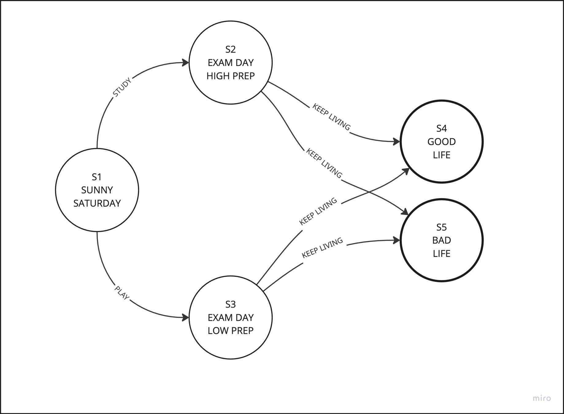
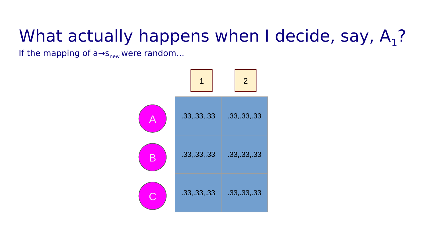
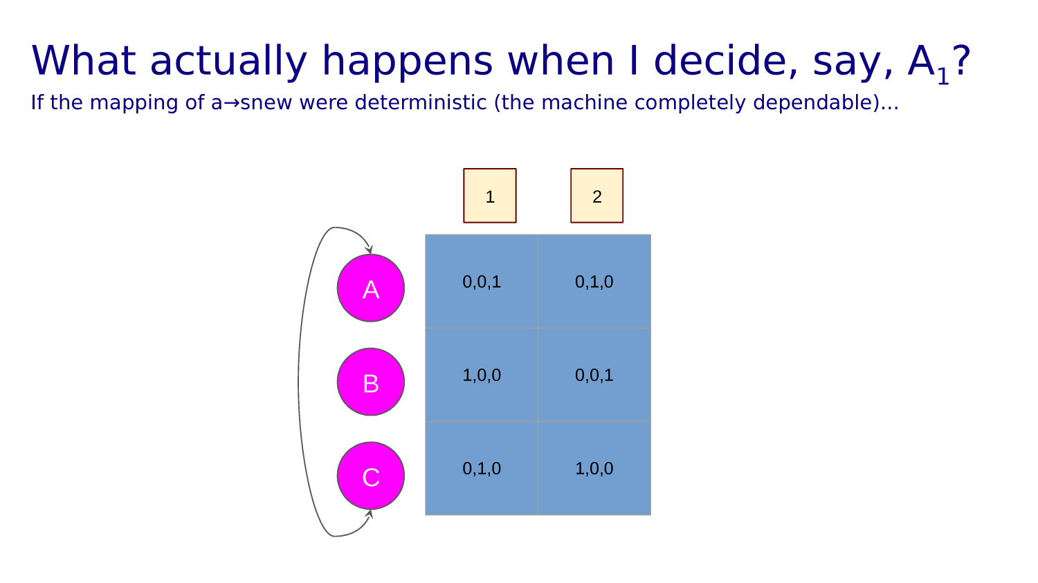
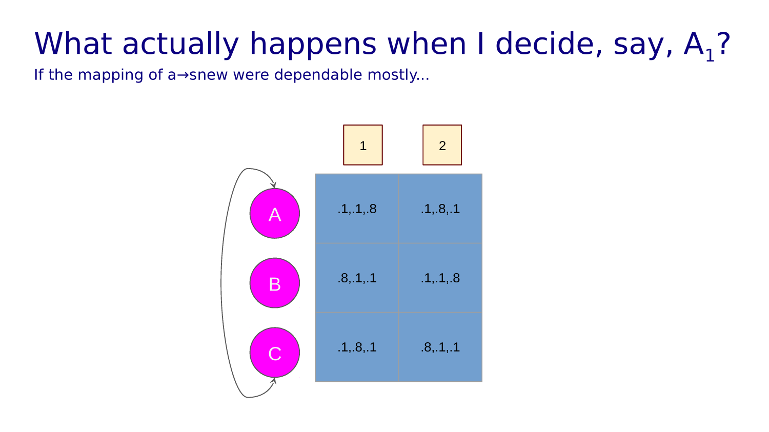
CHOOSE

ACTION A

CHOOSE

ACTION B

Stuff Happens

Make Decisions

Stuff Happens

You choose an action.

And stuff happens.

You choose another action.

And more stuff happens.

Current policy in this state

"Quality" of this state

R=+1.0

R=-1.0

-1.0

+1.0

-1.0

R=+1.0

R=-1.0

-1.0

+1.0

-1.0

0.0 -0.9

+0.9

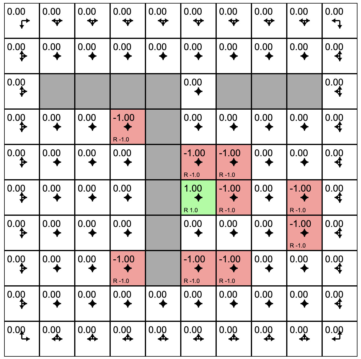
10x10 GridWorld

Policy Evaluation (one sweep)

P(a,s) = [0.25, 0.25, 0.25, 0.25, 0.25, 0.25, 0.25, 0.25, 0.25,
          0.25, 0.25, 0.25, 0.25, 0.25, 0.25, 0.25, 0.25, 0.25,
          0.25, 0.25, 0.25, 0.25, 0.25, 0.25, 0.25, 0.25, 0.25,
          0.25, 0.25, 0.25, 0.25, 0.25, 0.25, 0.25, 0.25, 0.25]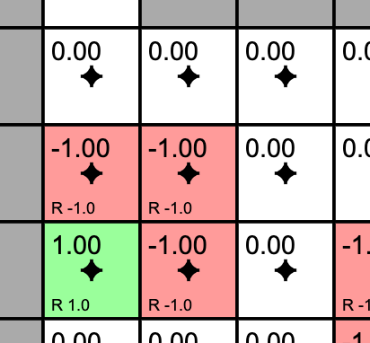

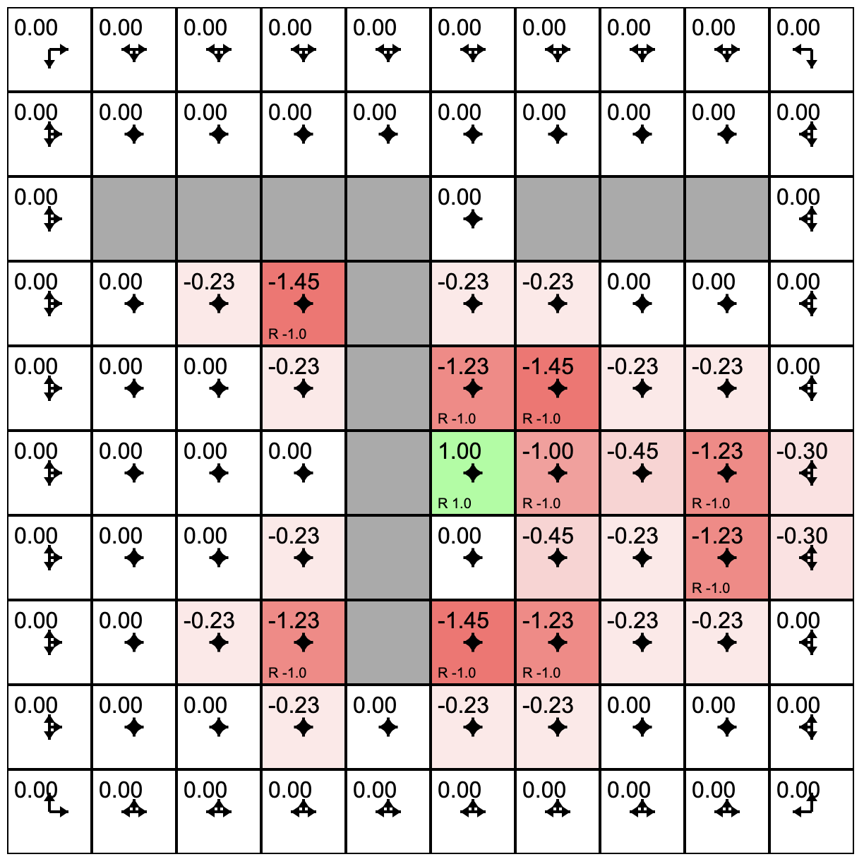
\text{Initial Policy, }\pi(s,a), \text{ is random - each action equally likely.}

Q of each state is just equal to the reward of that state

so, the actions yield 0, -.23, +.23, and -.23 so new Q is -1.23

Initial Condition

1 policy evaluation

R=-1.0

R=1.0

0 1 2

3 4 5

6 7 8

actions = [0, 1, 2, 3]     // L, U, R, D

s'(a,s) = [[0, 0, 1, 3],

           [0, 1, 2, 4],
           [1, 2, 2, 5],

           [3, 0, 4, 6],

           [3, 1, 5, 7],

           [6, 3, 7, 6],

           [6, 4, 8, 7],

           [7, 5, 8, 8]]

r(s) = [0, 0, 0, -1, -1, 0, 1, -1, 0]

V(s) = [0, 0, 0, 0, 0, 0, 0, 0, 0]

P(a,s) = [0.25, 0.25, 0.25, 0.25, 0.25, 0.25, 0.25, 0.25, 0.25,
          0.25, 0.25, 0.25, 0.25, 0.25, 0.25, 0.25, 0.25, 0.25,
          0.25, 0.25, 0.25, 0.25, 0.25, 0.25, 0.25, 0.25, 0.25,
          0.25, 0.25, 0.25, 0.25, 0.25, 0.25, 0.25, 0.25, 0.25]

evaluatePolicy: function() {
  var Vnew = zeros(numStates);                    // initialize new value array: 0 for each state
  
  for(var s=0;s < numStates;s++) {                //loop over all states
    var val = 0.0;
    var possA = allowedActions(s);                // fetch all possible actions
    
    for(var i=0,n=possActions.length;i < n;i++) { //loop over all possible actions
      var a = possActions[i];
      var prob = P[a*this.numStates +s ];         // get probability of this action from flattened policy array
      var nextS = nextStateDistribution(s,a);     // look up the next state
      var rs = reward(s,a,ns);                    // get reward for s->a->ns transition
      v += prob * (rs + gamma * V[nextS]);        //expected discounted reward from this action
    }
    
    Vnew[s] = v;                                  // record new value in value array
  }
  V = Vnew;                                       // swap old value array for new
},

Q of each state is just equal to the reward of that state

policy in this state is .25 in every direction

left is blocked so we stay in this state, up has no reward, right has R=-1, D has R=1.

0.25x1x0.9=.225= ~.23

so, the actions yield 0, -.23, +.23, and -.23 so new Q is -1.23

Initial Condition

1 policy evaluation

2 policy evaluations

R=-1.0

R=1.0

0 1 2

3 4 5

6 7 8

actions = [0, 1, 2, 3]     // L, U, R, D

s'(a,s) = [[0, 0, 1, 3],

           [0, 1, 2, 4],
           [1, 2, 2, 5],

           [3, 0, 4, 6],

           [3, 1, 5, 7],

           [6, 3, 7, 6],

           [6, 4, 8, 7],

           [7, 5, 8, 8]]

r(s) = [0, 0, 0, -1, -1, 0, 1, -1, 0]

V(s) = [0, 0, 0, 0, 0, 0, 0, 0, 0]

P(a,s) = [0.25, 0.25, 0.25, 0.25, 0.25, 0.25, 0.25, 0.25, 0.25,
          0.25, 0.25, 0.25, 0.25, 0.25, 0.25, 0.25, 0.25, 0.25,
          0.25, 0.25, 0.25, 0.25, 0.25, 0.25, 0.25, 0.25, 0.25,
          0.25, 0.25, 0.25, 0.25, 0.25, 0.25, 0.25, 0.25, 0.25]

evaluatePolicy: function() {
  var Vnew = zeros(this.ns); // initialize new value function array: 0 for each state
  
  for(var s=0;s < numStates;s++) { //loop over all states
    var val = 0.0;
    var possA = this.env.allowedActions(s); // fetch all possible actions
    
    for(var i=0,n=possA.length;i < n;i++) { //loop over all possible actions
      var a = possA[i];
      var prob = P[a*this.ns+s]; // get probability of this action from flattened policy array
      var nextS = nextStateDistribution(s,a); // look up the next state
      var rs = reward(s,a,ns); // get reward for s->a->ns transition
      v += prob * (rs + gamma * V[nextS]); //expected discounted reward from this action
    }
    
    Vnew[s] = v; // record new value in value array
  }
  this.V = Vnew; // swap old value array for new
},

Q of each state is just equal to the reward of that state

Initial Condition

1 policy evaluation

1 policy update

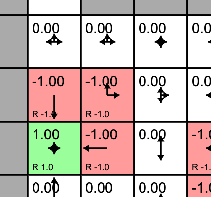
Policy here is updated from random

L and D options have Q=-1.0, U and R have 0.0

New policy here is U=0.5, R=0.5

Iterative Learning

Evaluate

Recalculate expected reward from this state based on current policy here and current quality of next states

Upate

Reset policy based on best alternative next states

One Policy Evaluation

One Policy Update

Three Policy Evaluations

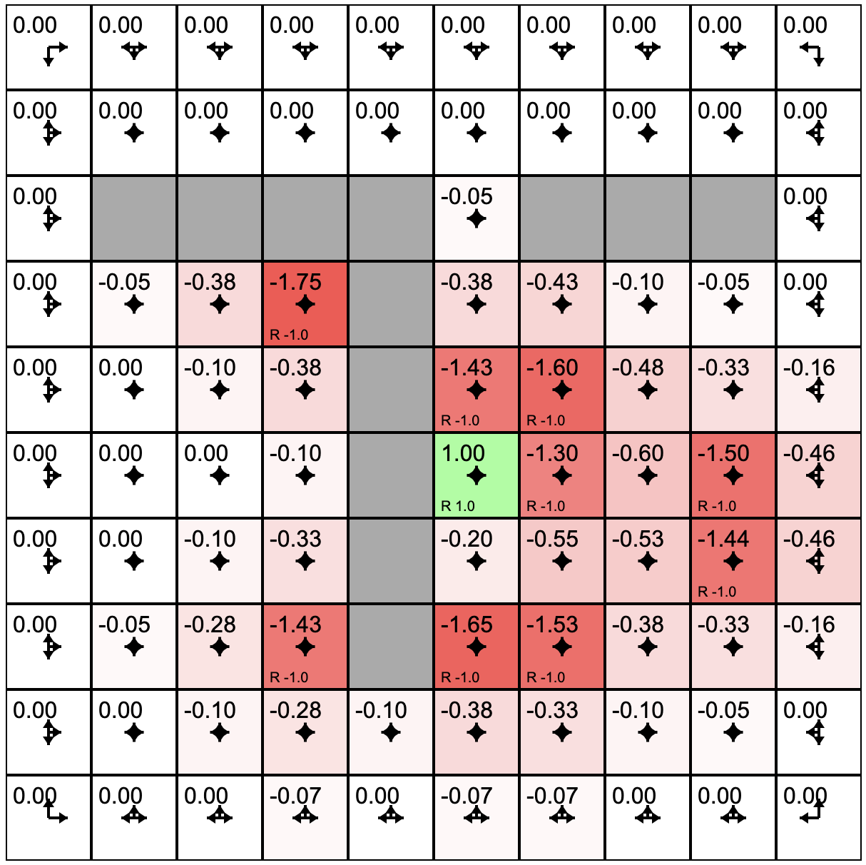
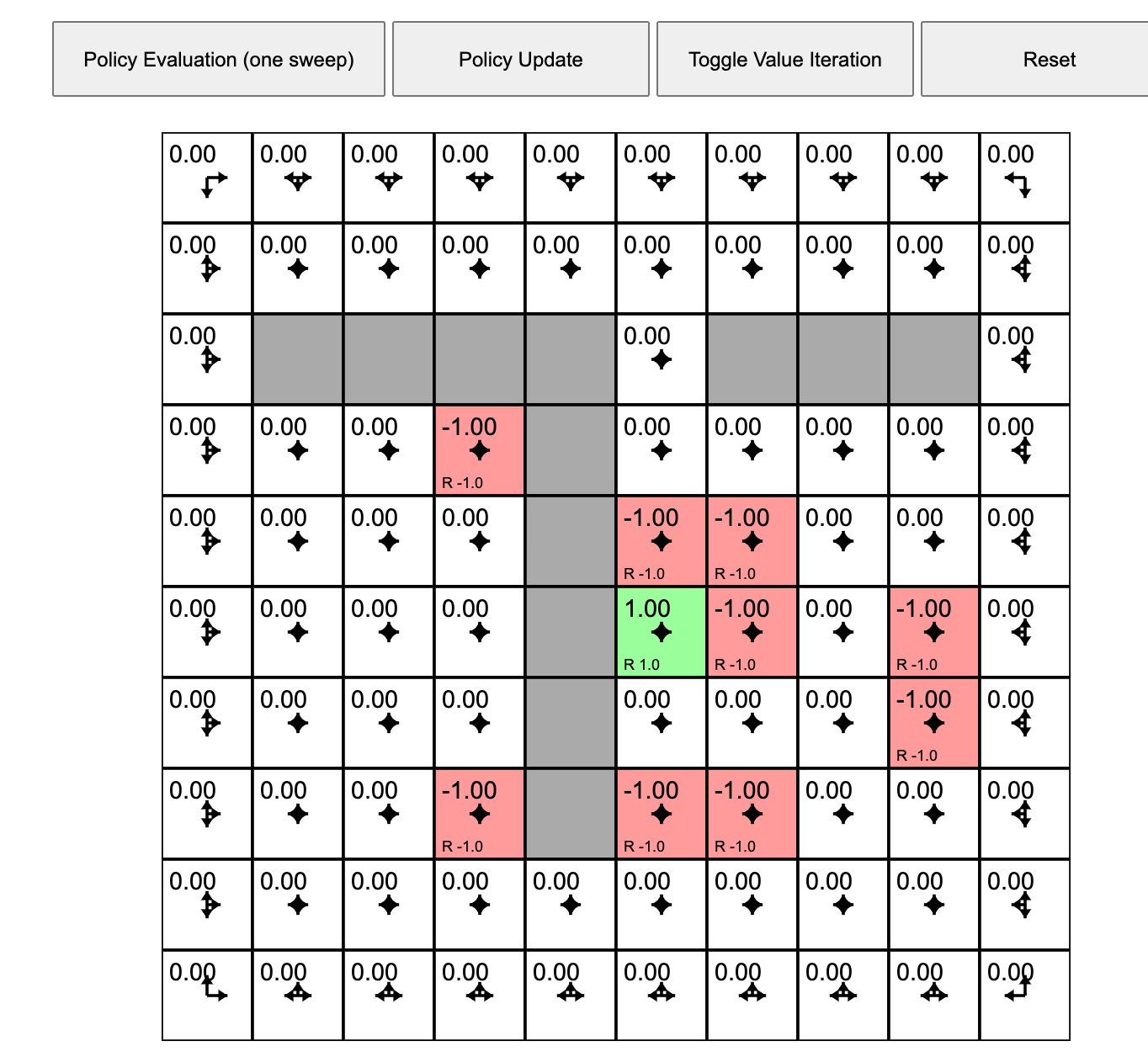
How It Works

Initial agent with a policy that treats all possible actions as equally likely.
Click "Policy Evaluation." This causes the agent to estimate the quality or value of each grid square under the current policy.
Click "Policy Update." This causes the agent to adjust its policy in the direction of better rewards based on its experience of the environment.
Clicking "Toggle Value Iteration" to turn on a continues sequence of policy evaluation followed by policy update.
1. As this runs you will see the arrows in each cell adjust. The length of the arrow shows the likelihood of choosing to move in that direction under the current policy.
The slider at the bottom allows you to tweak the rewards/punishments associated with each state. To do this, click on the state and then adjust the slider.
You can experiment with the model by training it (toggle the value iteration on until it settles) and then sprinkle positive and negative rewards in the state space. If value iteration is still on it will immediately find a policy that takes these into account. If value iteration was off, you can switch it on to watch the model adjust. Try putting up barriers by making blocks of highly negative rewards.

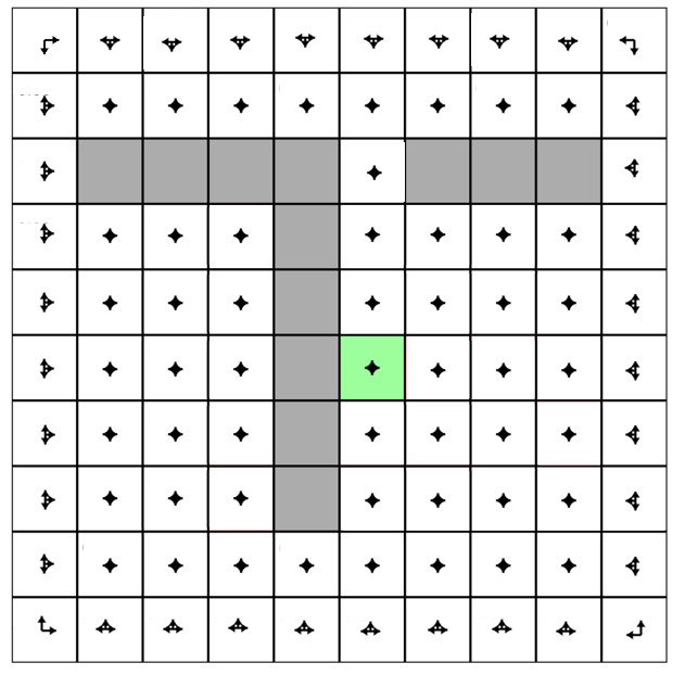
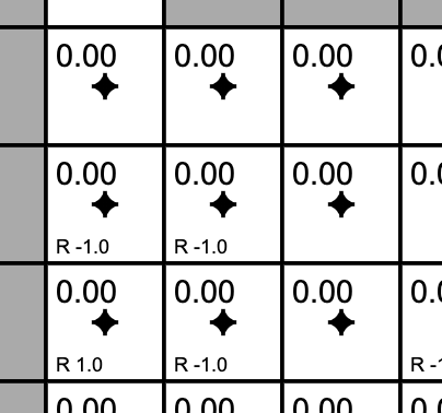
one more thing...

https://cs.stanford.edu/people/karpathy/reinforcejs/gridworld_dp.html

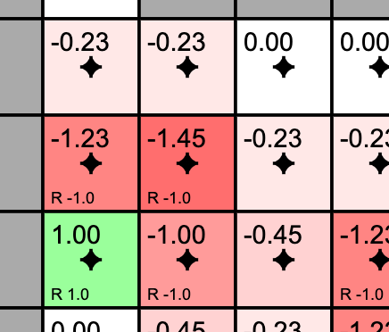
STOP+THINK

One policy evaluation step has assigned values to the states that have rewards in them. And then the agent's policy was updated.

Consider the state outlined in purple. What will its value be if we evaluate the current policy?

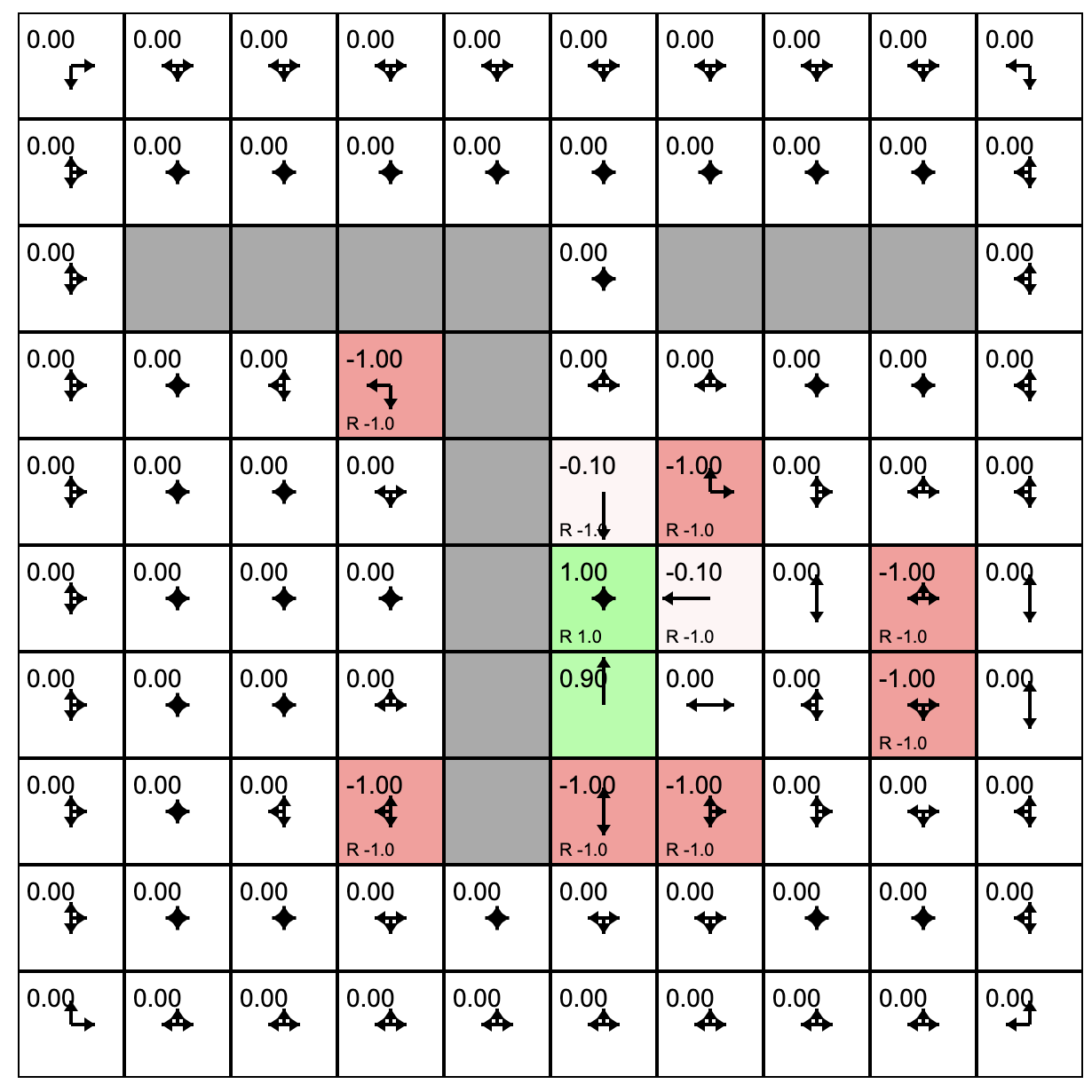
The state's previous value was -1.0. The policy for this state has only one option: down. Following this policy lands us in a state with reward 1.0. But this state is one step away so we discount the reward with gamma=0.9. The result is -1.0 + 0.9 = 0.1.

NOTES

singularity

ASI

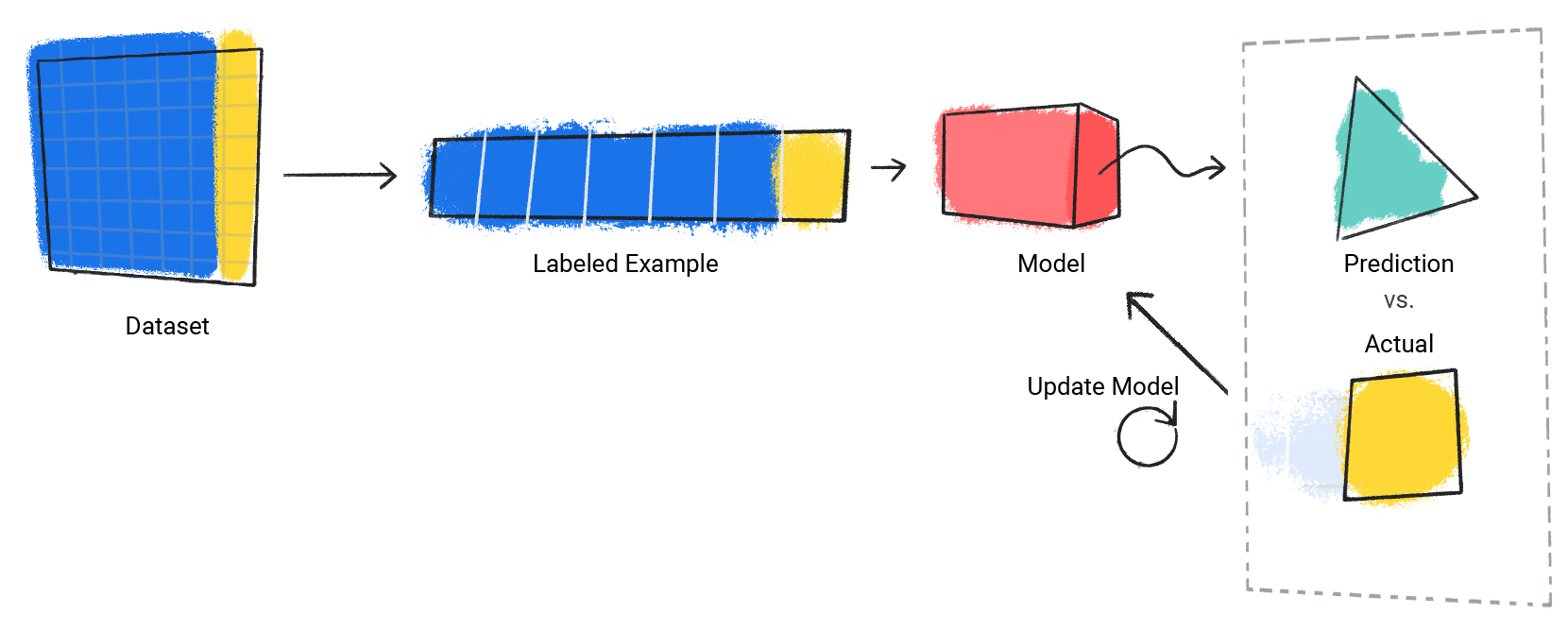
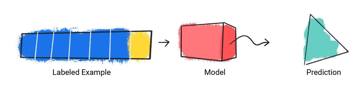
training

labels

prediction

training data

training set

model parameters

loss, cost, error

over-, underfitting

bias

variance

Bias-Variance Tradeoff

overfitting - more training data

overfitting regularization

hyper-parameter

cross-validation

Text

singularity

ASI

training

labels

prediction

training data

training set

model parameters

loss, cost, error

over-, underfitting

bias

variance

Bias-Variance Tradeoff

overfitting - more training data

overfitting regularization

hyper-parameter

cross-validation

Text

REFERENCES

IMAGES

#FromLastWeek

Learn more about Learning

Teaser: Cooperative Learning Agents

Driving Marshmallows Grad School

WHAT'S
GOING
ON?

WHAT IS HAPPENING WHEN WE
DEFER
GRATI
FICA
TION?

WHY ARE YOU
DOING
THIS?

	A
D	NOW	B
	C

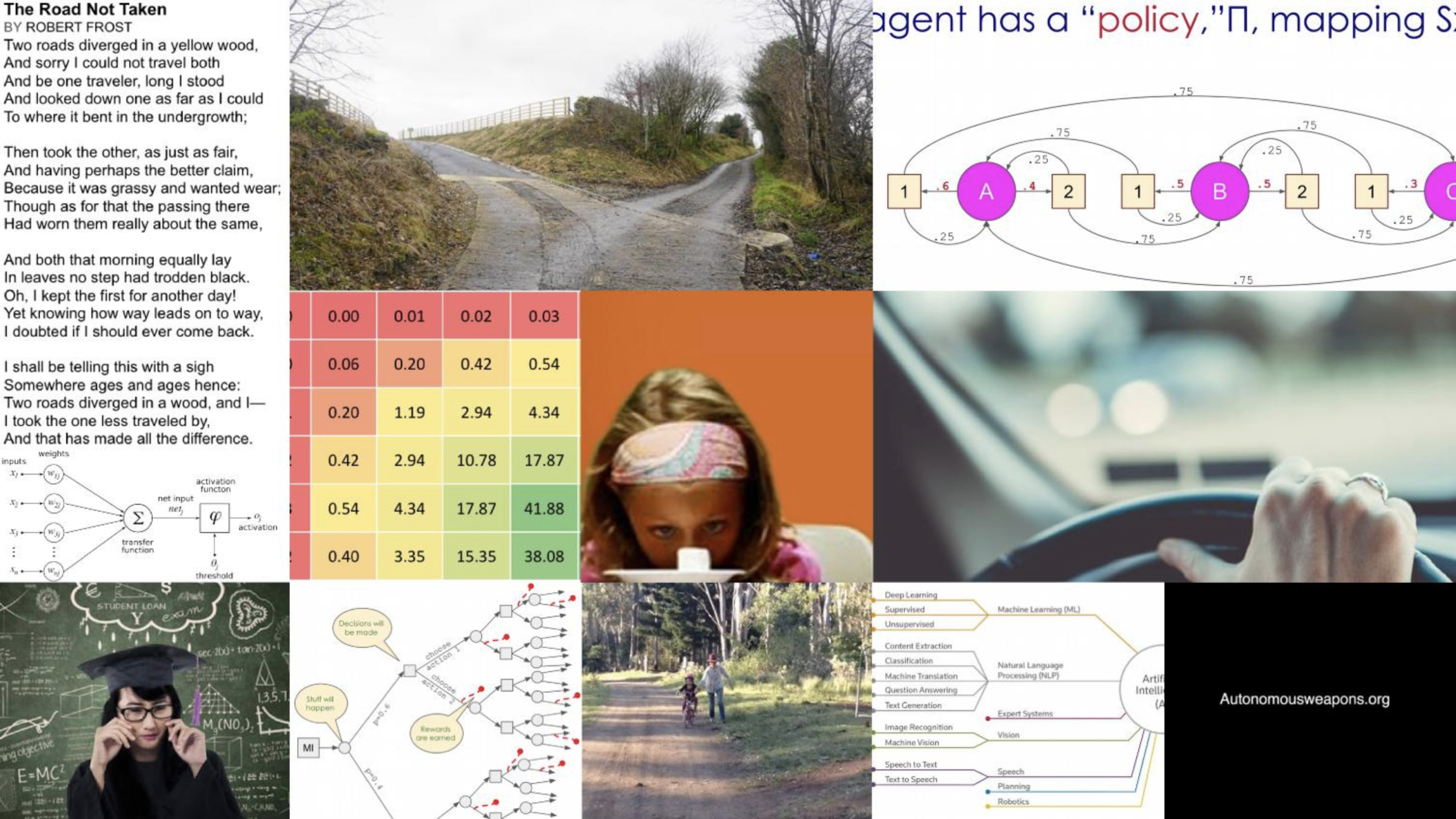
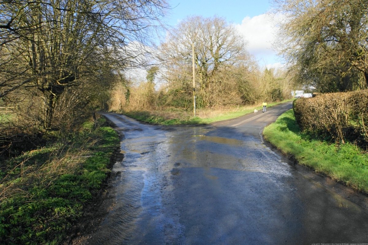
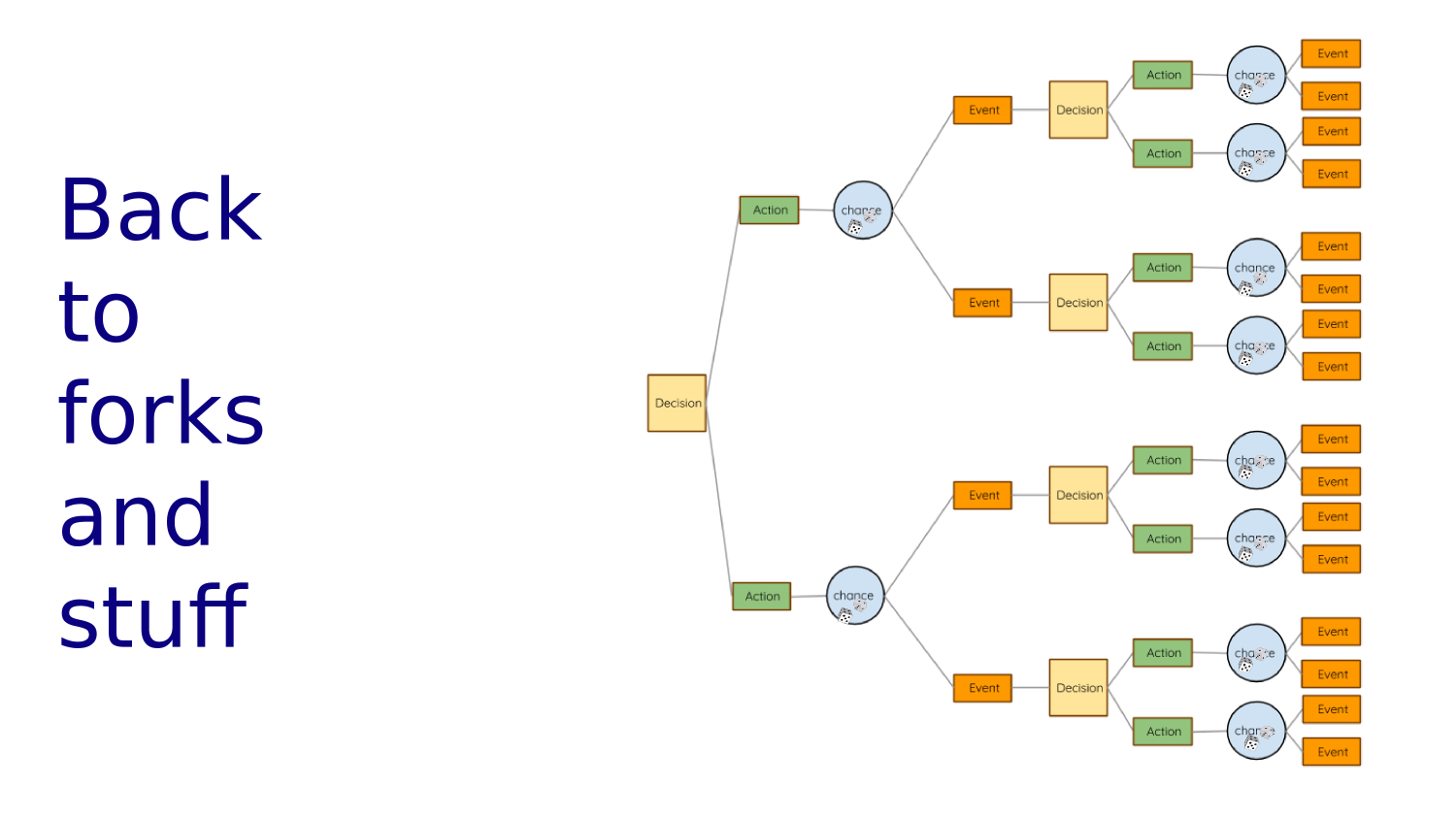
Forks in the Road

Choosing at Forks in the Road

The Road Not Taken
BY ROBERT FROST
Two roads diverged in a yellow wood,
And sorry I could not travel both
And be one traveler, long I stood
And looked down one as far as I could
To where it bent in the undergrowth;

Then took the other, as just as fair,
And having perhaps the better claim,
Because it was grassy and wanted wear;
Though as for that the passing there
Had worn them really about the same,

And both that morning equally lay
In leaves no step had trodden black.
Oh, I kept the first for another day!
Yet knowing how way leads on to way,
I doubted if I should ever come back.

I shall be telling this with a sigh
Somewhere ages and ages hence:
Two roads diverged in a wood, and I—
I took the one less traveled by,
And that has made all the difference.

Road junction in Bury Green Millfield Lane is left while Cradle End is to the right. Both lead to the A120. Bill Boaden CC BY-SA 2.0

https://www.nytimes.com/2021/05/14/books/visualizing-robert-frosts-seminal-poem.html

STOP+THINK

Did it make ALL the difference?

Living is One Fork in the Road After Another

https://devblogs.nvidia.com/deep-learning-nutshell-reinforcement-learning/ (Video courtesy of Mark Harris, who says he is “learning reinforcement” as a parent.)

Tim Dettmers 2016 "Deep Learning in a Nutshell: Reinforcement Learning"

STOP+THINK

What else about learning to ride a bike strikes you as interesting? Do you think it's important that it's fun? Is it important that mom is there?

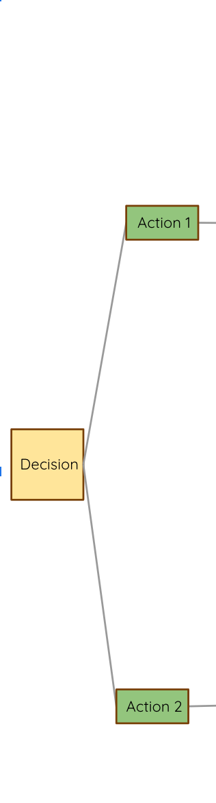
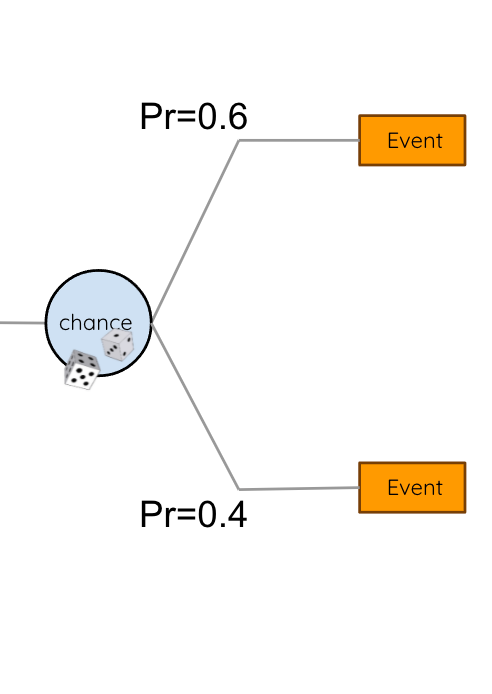
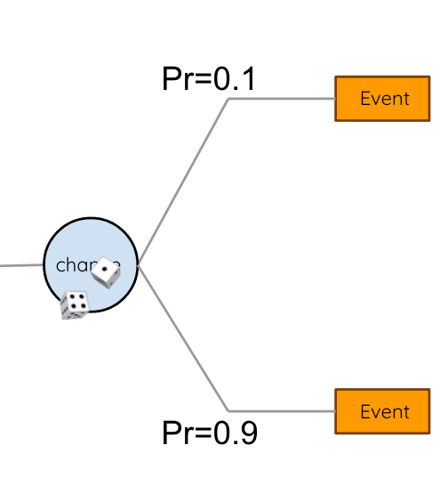
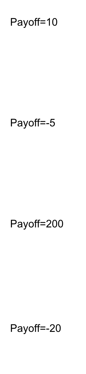
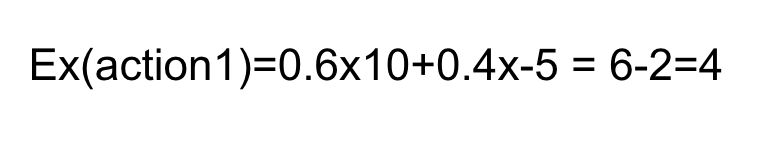
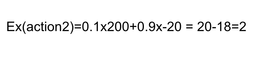
The EXPECTED VALUE of a decision/action is the sum of the possible outcomes weighted by their likelihood

We can choose between actions based on their expected value. Here we choose action 1.

WHAT IS HAPPENING WHEN WE
DEFER
GRATI
FICA
TION?

Time is Money.

"Advice to a Young Tradesman", Benjamin Franklin

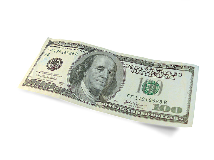
https://www.pickpik.com/

Would you rather have 100 dollars today or two years from now?

How about 80 dollars today or 100 dollars two years from now?

How about 90?

Discounting

How to Decide?

It's just compound interest in reverse

Discounting

B_{n}\ =(1+r)^n B_{0}

B_{0}=B_n\frac{1}{(1+r)^n}

"The future balance in year n of starting balance B₀ is ..."

"The discounted value future balance Bn is that value times gamma to the n"

It's just compound interest in reverse

1 plus interest rate raised to the nth power times the initial balance

Rearrange to express current balance in terms of future balance

B_{0}=B_n\frac{1}{(1+r)^n}=B_n\gamma^n

Reward_now = 0.9¹⁰ x 1000 = 349

Assume gamma = 0.9

Discounting Example

Reward_now = 0.9¹⁴ x 1000 = 227

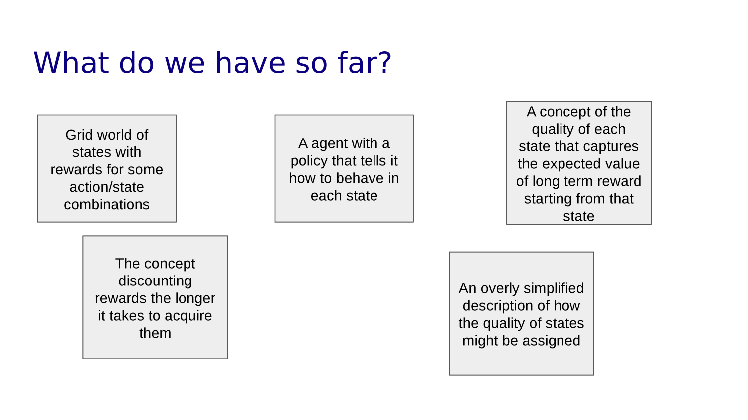
So far

the probabilities of downstream rewards

AND

is related to

in gridworld

of an action

The expected value

the length of the paths to those rewards.

Life is one decision after another

Decisions
have
consequences

But, some consequences are more likely than others.

"I returned, and saw under the sun, that the race is not to the swift, not the battle to the strong, neither yet bread to the wise, nor yet riches to men of understanding, nor yet favour to men of skill; but time and chance happeneth to them all."

Ecclesiastes 9:11, King James Version

In other words...
SHIT HAPPENS.

Simplify Things

GRIDWORLD

Imagine life as movement in a chess board world. Each square is a "state" and we choose one of four actions: move, one square at time, UP, DOWN, LEFT, or RIGHT.

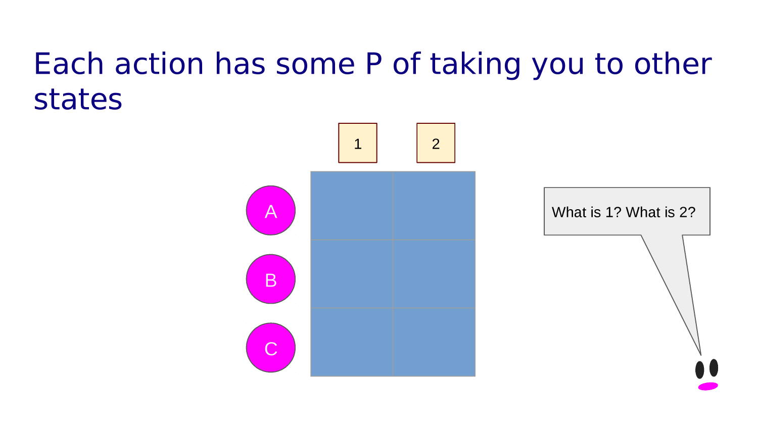
Actions take
us from state to state

0.5

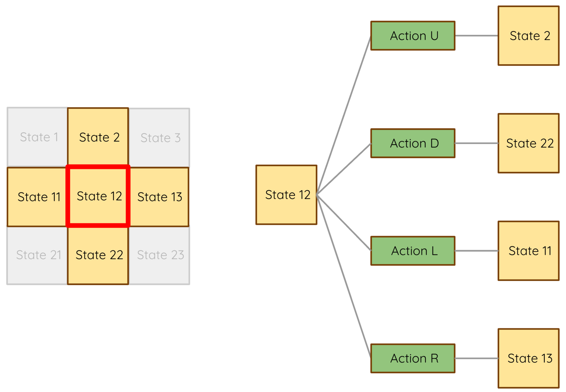
Choosing Among Options: Policy

0.25

0.00

Read: 50% of the time I go UP, 25% of the time I go DOWN, 25% of the time I go RIGHT. I never go LEFT.

Policy(state 12) = {0.5,0.25, 0, 0.25)

0.5

Choosing Among Options: Policy

0.25

0.0

Policy(state 12) = {0.5,0.25, 0, 0.25)

reward=10

reward=0

reward=-4

Ex(Policy(state 12)) = 0.5x10+0.25x(-4)=4

Takeaways So Far

The "value" of a choice at a fork in the road is its expected value - the weighted average of the things life paths that start with heading down that fork.

We can simplify life and think of it as moving around on a chess board.

A policy is a list of how likely we choose which actions in a given state.

We can compute the value of a policy in a given state.

One More New Concept...

Gridworld

1	2	3	4	5	6	7
8	9	10			13	14
15	16	17	18	19	20	21
22	23	24	25	26	27	28
29		31		33	34	35
36		38		40	41	42
43	44	45	46	47	48	49

start here

end here

walls/obstacles - can't go here

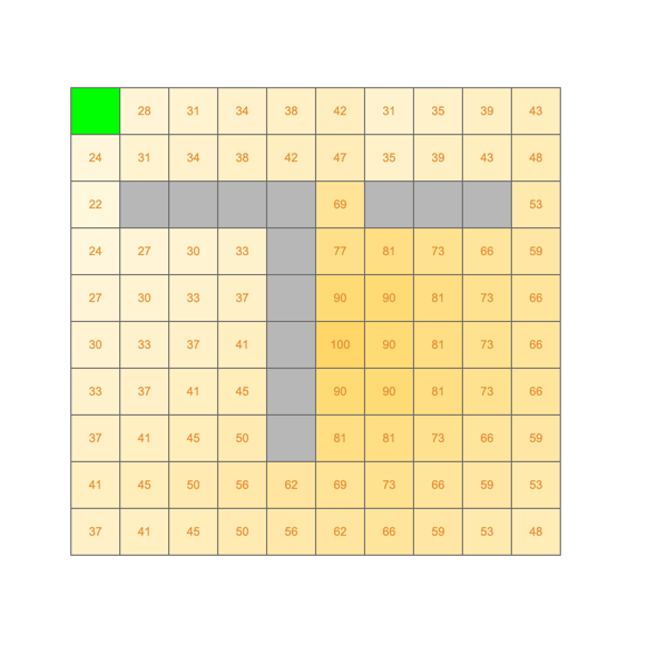
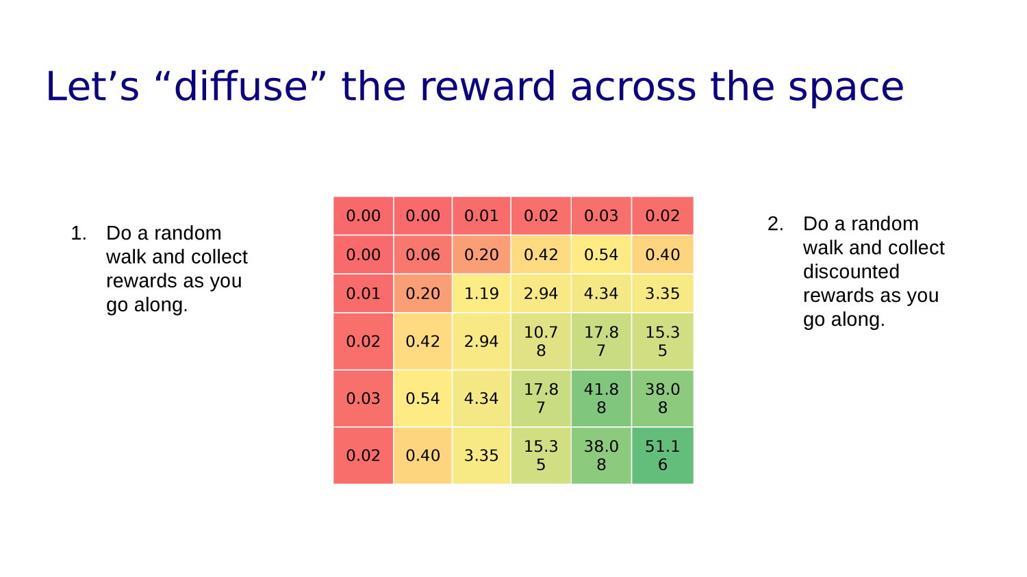
"Diffuse" the Reward

Assume reward at goal







						100

100x0.9=90

53x0.9=48

48x0.9=43

35x0.9=31

90x0.9=81

81x0.9=73

73x0.9=66

66x0.9=59

59x0.9=53

43=0.9=39

39x0.9=35

31x0.9=28

This sort of^* says "the expected reward averaged over all the paths that start out in the upper left state is 28.

* not quite, though, because we haven't taken into account all the wandering paths we could take

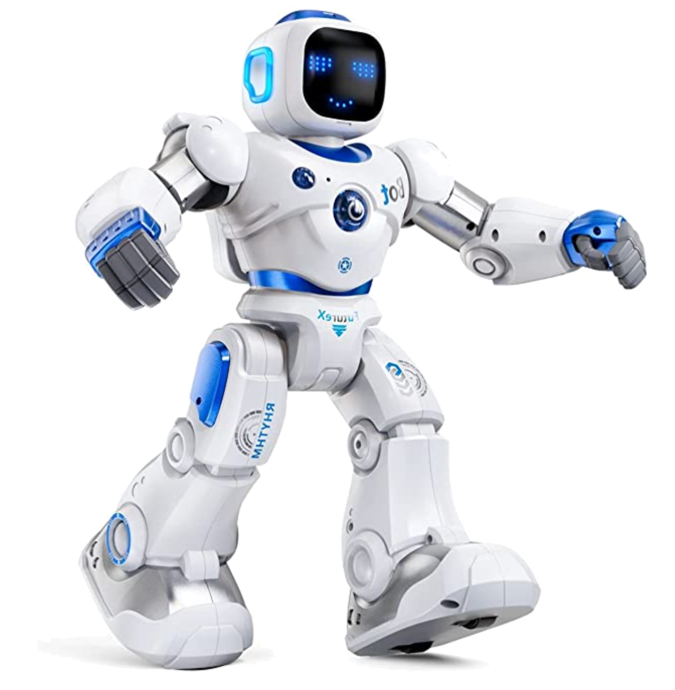
Could a robot learn the best path?







						100

Questions?

How can we automate making good decisions at repeated forks in the road?

Rewards

Groundhog Day

Try out everything over and over and over again and keep track of how everything works out each time.

The Plan

Putting it all together

A grid of STATES

a set of actions

S = {s₁, s₂, ..., s_n}

A = {a₁, a₂, a₃, a₄}

19	13	25	20	X
20	14	26	21	19
21	15	27	22	20
22	16	28	23	21
23	17	9	24	22
24	18	30	X	23
25	19	31	26	X
26	20	32	27	25
27	21	33	28	26
28	22	34	29	27
29	23	35	30	28
30	24	36	X	29
31	25	X	32	X
32	26	X	33	32
33	27	X	34	33
34	28	X	35	34
35	29	X	36	35
36	30	X	X	35

1	X	7	2	X
2	X	8	3	1
3	X	9	4	2
4	X	10	5	3
5	X	11	6	4
6	X	12	X	5
7	1	13	8	X
8	2	14	9	7
9	3	15	10	8
10	4	16	11	9
11	5	17	12	10
12	6	18	X	11
13	7	19	14	X
14	8	20	15	13
15	9	21	16	14
16	10	22	17	15
17	11	23	18	16
18	12	24	X	17

STATE	U	D	R	L

STATE	U	D	R	L

ACTION

States
and
Actions
and
Policies

In each state an action takes me to another state.

The rule I use for choosing actions in each state is my policy.

For example: mostly I go down, sometimes right or up, rarely left.

Start Simple: Random Policy

STATE	UP	DOWN	LEFT	RIGHT
1	0	.5	0	.5
2	0	.33	.33	.33
3	0	.33	.33	.33
4	0	.33	.33	.33
5	0	.33	.33	.33
6	0	.5	.5	0
...	...	...	...	...

1	2	3	4	5	6

Data Jig for Policy - array of arrays?

policy = [ [0, 0.5, 0.5, 0],

           [0, 0.33, 0.33, 0.33],

           [0, 0.33, 0.33, 0.33],

           [0, 0.33, 0.33, 0.33],

           [0, 0.33, 0.33, 0.33],

           [0, 0.5, 0.5, 0]

...

]

Looks a bit like "weights" from last week, eh?

Can We Do Better Than Random Policy?

Reinforcement
Learning

Repeat a task many times to determine a policy that will maximize the expected reward.

Recall

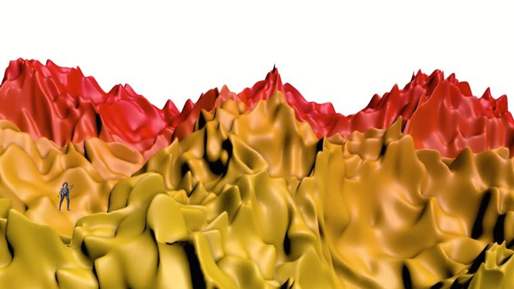
Our discussion of "points" in a solution space.

What combination of, say, Kp, Ki, Kd yield the minimal error?

What combination of weights in a neural network yield best predictions?

What combination of actions in states (policy) yields the highest reward?

Reinforcement
Learning

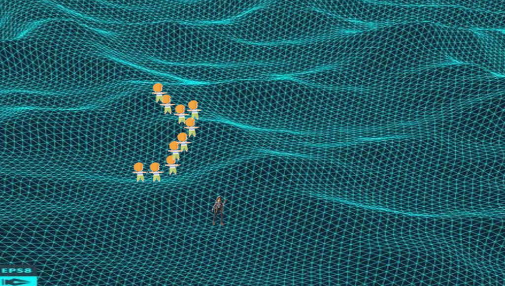
For computer vision some of the readings introduced the idea of "gradient descent" - learning by moving in "weight landscape" toward weight combinations that reduced the cost/loss.

HERE, the learning proceeds by moving in the direction of increasing reward on the policy landscape.

Finis

https://innoeduvation.org/313/learn/RL-Karpathy/reinforcejs-master/gridworld_td.html

Out Takes

The Grid of My Life

URHERE

Each state has a "quality" Q based on expected value of rest-of-your-life paths that start there

What's your policy? How has it evolved? Remember not to play it too safely!

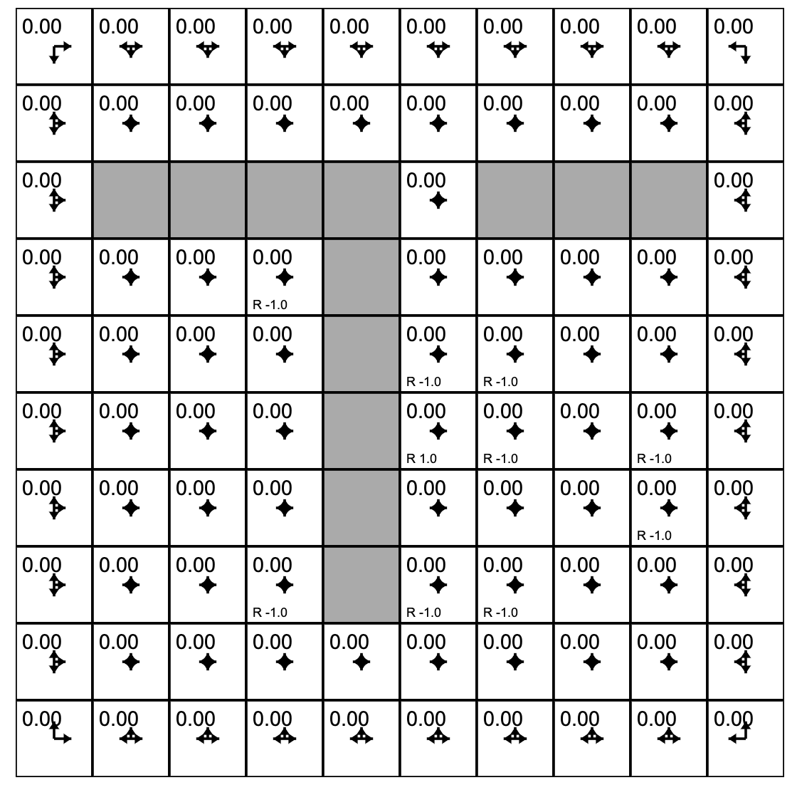
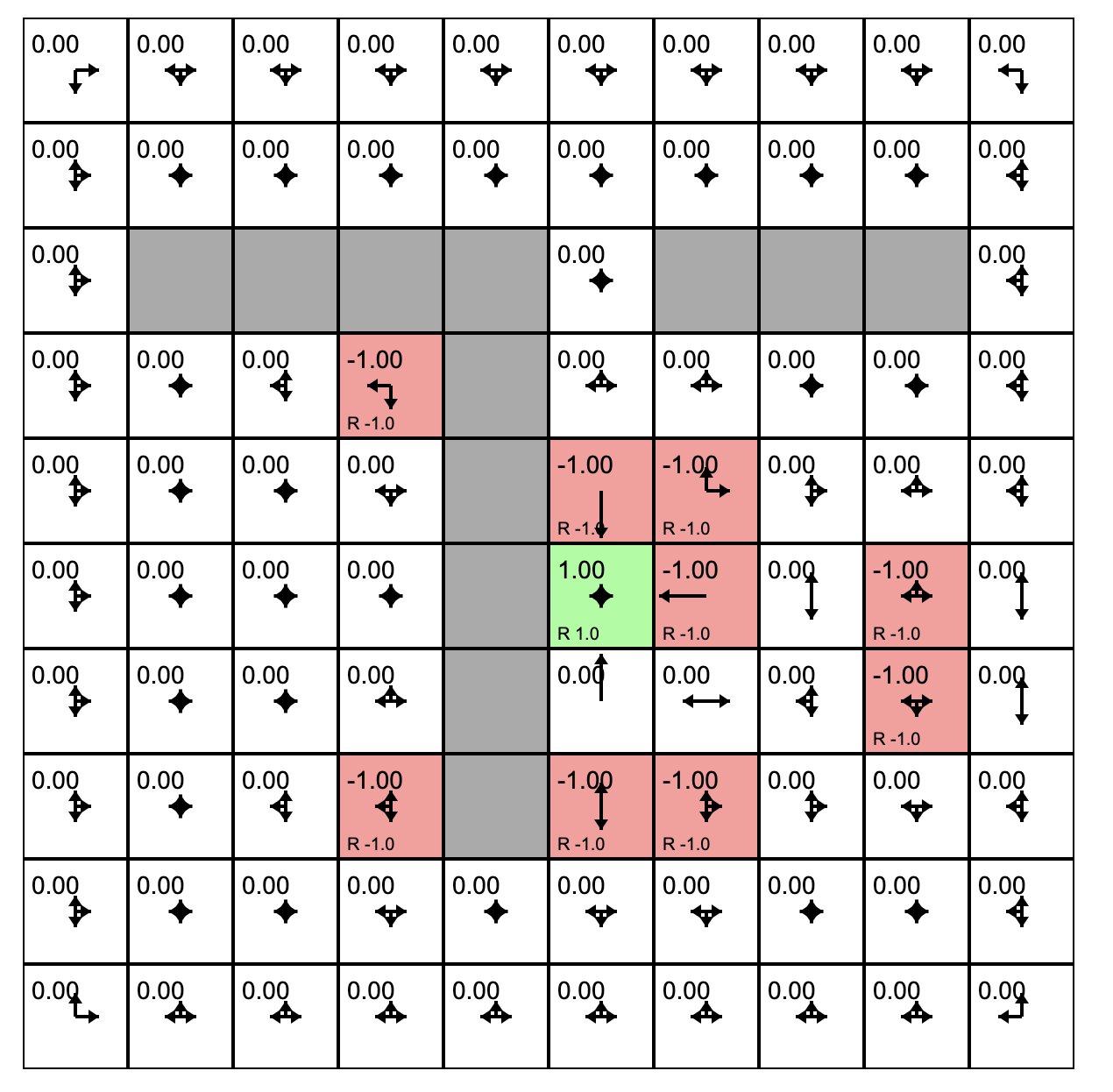
Reinforcement Learning in Gridworld

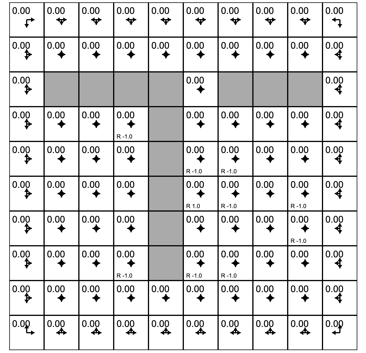
Let's play with Andrej Karpathy (Links to an external site.)'s Gridworld RL simulation written using the ReinforceJS library. The next few paragraphs paraphrase his text. The simulation takes place in what we call a "toy environment" called Gridworld - a rectangle of squares on which an "agent" can move. Each square represents a state. One square (upper left) is the start square. Another square is the goal square. In this particular simulation:

The world has 10x10 = 100 distinct states. Gray cells are walls that block the agent.
The agent can choose from 4 actions up, down, right, left. The probability of each action under the current policy is shown by the size of an arrow emanating from the center of each square.
This world is deterministic - if an agent chooses the action "move right" it will transition to the state to the right.
The agent receives +1 reward when it reaches the center square (rewards are indicated at the bottom of each square as, for example, R 1.0), and -1 reward in a few states. The state with +1.0 reward is the goal state and resets the agent back to start.
A slider below the grid allows the user to set the reward for each state: click on the state and then adjust the slider.

In other words, this is a deterministic, finite Markov Decision Process (MDP) and as always the goal is to find an agent policy (shown here by arrows) that maximizes the future discounted reward. My favorite part is letting Value iteration converge, then change the cell rewards and watch the policy adjust.

Interface. The color of the cells (initially all white) shows the current estimate of the Value (discounted reward) of that state, with the current policy. Note that you can select any cell and change its reward with the Cell reward slider.

Text

Next Time

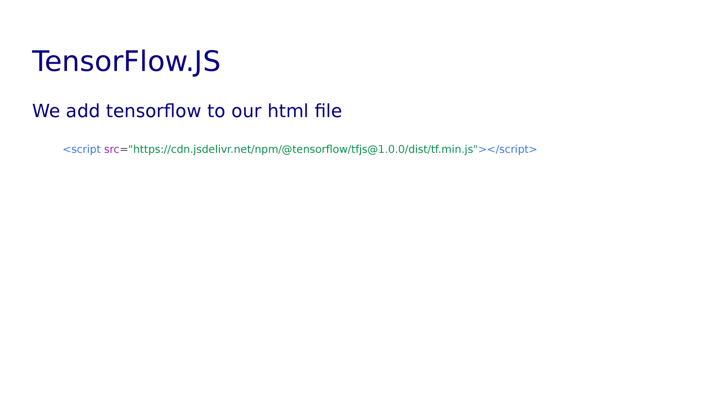
Tensorflow

Google's AI/ML platform

"Competitors": OpenCV, Caffe2, pyTorch, Keras, and many more

What is a Tensor?

scalar

vector

matrix

\begin{bmatrix} w_{1,1} & w_{1,2} & w_{1,3} \\ w_{2,1} & w_{2,21} &w_{2,3} \end{bmatrix}

\begin{bmatrix} k_{p} \\ k_{i} \\ k_{d} \end{bmatrix}

\begin{bmatrix} m \end{bmatrix}

\begin{bmatrix} \begin{bmatrix} w_{1,1} \\ w_{2,1} \end{bmatrix} & \begin{bmatrix} w_{1,1} \\ w_{2,1} \end{bmatrix} & \begin{bmatrix} w_{1,1} \\ w_{2,1} \end{bmatrix} \\ \\ \begin{bmatrix} w_{1,1} \\ w_{2,1} \end{bmatrix} & \begin{bmatrix} w_{1,1} \\ w_{2,1} \end{bmatrix} & \begin{bmatrix} w_{1,1} \\ w_{2,1} \end{bmatrix} \end{bmatrix}

What is a Tensor?

References, etc.

What is a Tensor?

tensor

What is a Tensor?

Nodes have a weight for each input.

Layers have multiple nodes.

Models have multiple layers.

You get the picture.

What is a Tensor?

Resources

tensorflow.js

image classification

object detection

body segmentation

pose estimation

language embedding

speech recognition

tensorflow.js

Load data.
Define model "architecture"
Train model
Evaluate model

model architecture

```
model = tf.sequential();
```
```
model.add(tf.layers.conv2d...
```
```
model.add(tf.layers.maxPooling2d
```
```
model.add(tf.layers.conv2d...
```
```
model.add(tf.layers.maxPooling2d
```
```
model.add(tf.layers.flatten());
```
```
model.add(tf.layers.dense({
```

model architecture

https://www.jessicayung.com/explaining-tensorflow-code-for-a-convolutional-neural-network/

convolution

https://towardsdatascience.com/conv2d-to-finally-understand-what-happens-in-the-forward-pass-1bbaafb0b148

kernel

stride

Repetitions

https://www2.slideshare.net/samchoi7/tensorflow-tutorial-part1/8

flattening

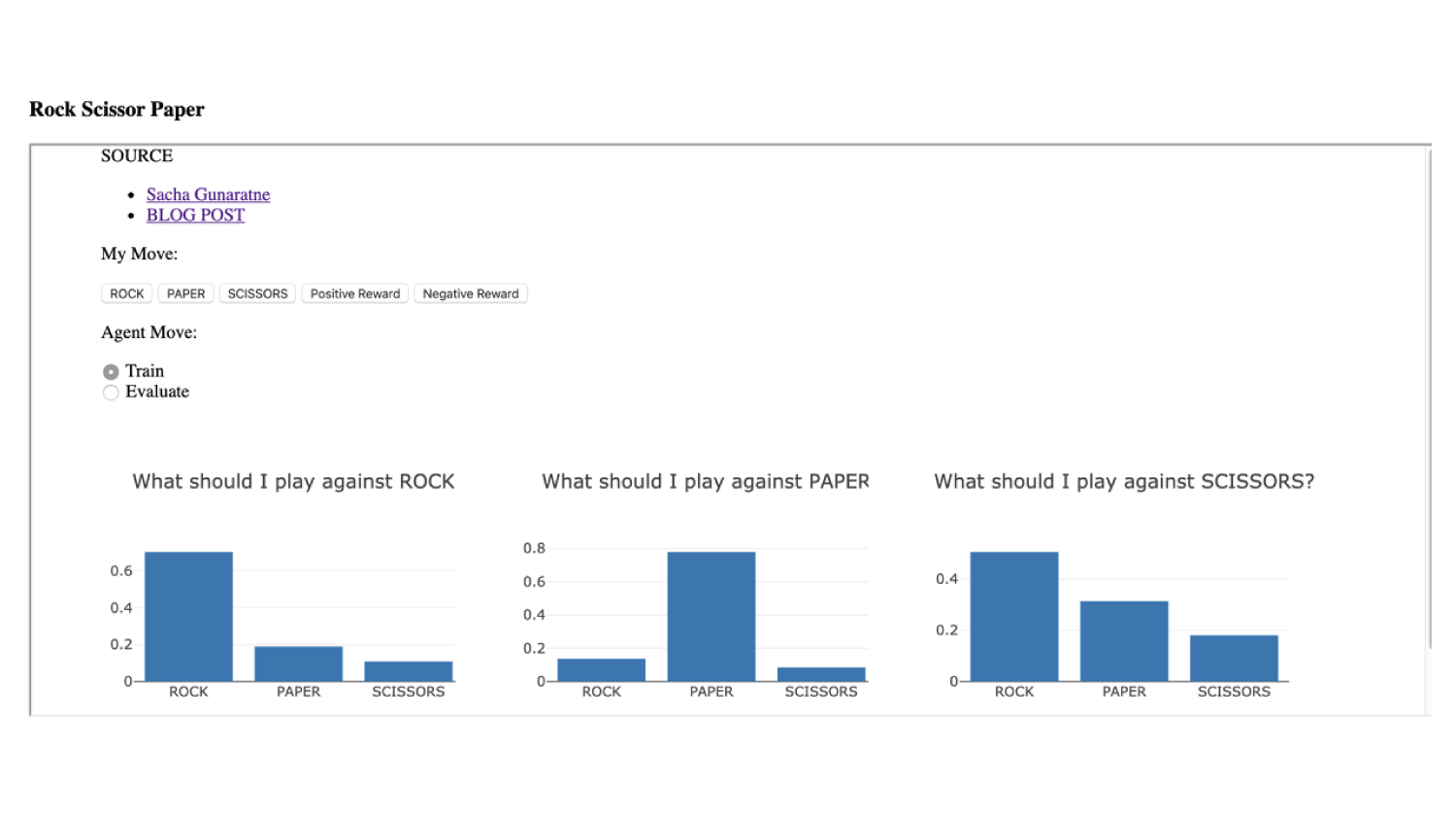
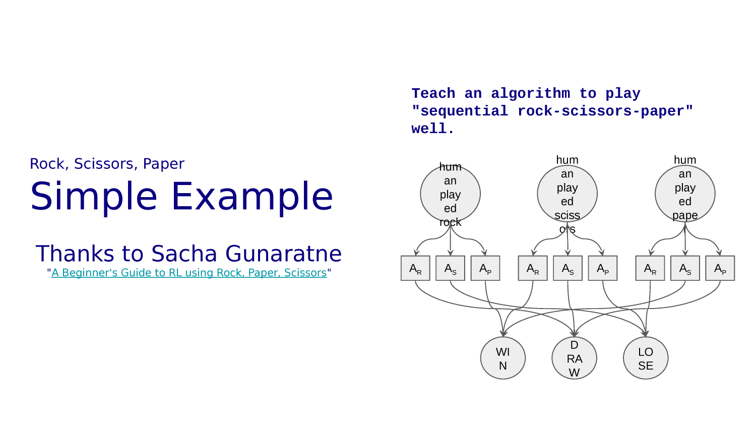
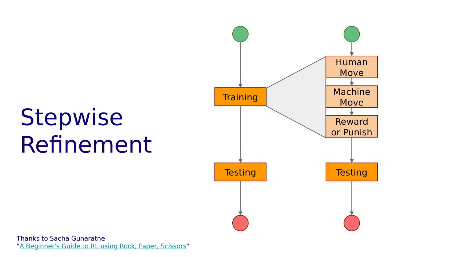
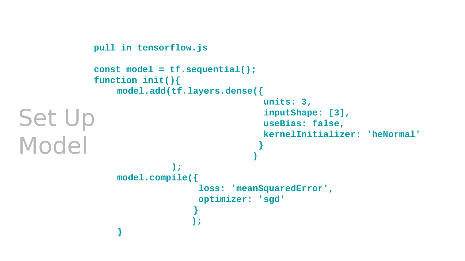
Multi-agent Reinforcement Learning
(MARL)

INF1339 W11 Lobby

0	1	2	3	4	5	6	7	8	9
10	11	12	13	14	15	16	17	18	19
20	21	22	23	24	25	26	27	28	29
30	31	32	33	34	35	36	37	38	39
40	41	42	43	44	45	46	47	48	49
50	51	52	53	54	55	56	57	58	59
60	61	62	63	64	65	66	67	68	69
70	71	72	73	74	75	76	77	78	79
80	81	82	83	84	85	86	87	88	89
90	91	92	93	94	95	96	97	98	99

1	2	3	4	5	6	7
8	9	10			13	14
15	16	17	18	19	20	21
22	23	24	25	26	27	28
29		31		33	34	35
36		38		40	41	42
43	44	45	46	47	48	49

19	13	25	20	X
20	14	26	21	19
21	15	27	22	20
22	16	28	23	21
23	17	9	24	22
24	18	30	X	23
25	19	31	26	X
26	20	32	27	25
27	21	33	28	26
28	22	34	29	27
29	23	35	30	28
30	24	36	X	29
31	25	X	32	X
32	26	X	33	32
33	27	X	34	33
34	28	X	35	34
35	29	X	36	35
36	30	X	X	35

1	X	7	2	X
2	X	8	3	1
3	X	9	4	2
4	X	10	5	3
5	X	11	6	4
6	X	12	X	5
7	1	13	8	X
8	2	14	9	7
9	3	15	10	8
10	4	16	11	9
11	5	17	12	10
12	6	18	X	11
13	7	19	14	X
14	8	20	15	13
15	9	21	16	14
16	10	22	17	15
17	11	23	18	16
18	12	24	X	17

STATE	UP	DOWN	LEFT	RIGHT
1	0	.5	0	.5
2	0	.33	.33	.33
3	0	.33	.33	.33
4	0	.33	.33	.33
5	0	.33	.33	.33
6	0	.5	.5	0
...	...	...	...	...

0	1	2	3	4	5	6	7	8	9
10	11	12	13	14	15	16	17	18	19
20	21	22	23	24	25	26	27	28	29
30	31	32	33	34	35	36	37	38	39
40	41	42	43	44	45	46	47	48	49
50	51	52	53	54	55	56	57	58	59
60	61	62	63	64	65	66	67	68	69
70	71	72	73	74	75	76	77	78	79
80	81	82	83	84	85	86	87	88	89
90	91	92	93	94	95	96	97	98	99

1	2	3	4	5	6	7
8	9	10			13	14
15	16	17	18	19	20	21
22	23	24	25	26	27	28
29		31		33	34	35
36		38		40	41	42
43	44	45	46	47	48	49

19	13	25	20	X
20	14	26	21	19
21	15	27	22	20
22	16	28	23	21
23	17	9	24	22
24	18	30	X	23
25	19	31	26	X
26	20	32	27	25
27	21	33	28	26
28	22	34	29	27
29	23	35	30	28
30	24	36	X	29
31	25	X	32	X
32	26	X	33	32
33	27	X	34	33
34	28	X	35	34
35	29	X	36	35
36	30	X	X	35

1	X	7	2	X
2	X	8	3	1
3	X	9	4	2
4	X	10	5	3
5	X	11	6	4
6	X	12	X	5
7	1	13	8	X
8	2	14	9	7
9	3	15	10	8
10	4	16	11	9
11	5	17	12	10
12	6	18	X	11
13	7	19	14	X
14	8	20	15	13
15	9	21	16	14
16	10	22	17	15
17	11	23	18	16
18	12	24	X	17

STATE	UP	DOWN	LEFT	RIGHT
1	0	.5	0	.5
2	0	.33	.33	.33
3	0	.33	.33	.33
4	0	.33	.33	.33
5	0	.33	.33	.33
6	0	.5	.5	0
...	...	...	...	...

HOW DO MACHINES LEARN I

OUTTAKES

mea culpa

ISCHOOL VISUAL IDENTITY

INTRO

max pooling

Pooling and Convolutions are two families of filters. There are others...

Supervised Learning

Great Quick Course

Classification

Binary Classification

(Unsupervised Learning)

HOW DO MACHINES LEARN II (DL)

Deep Learning (DL)

Other Model Architectures

HOW DO MACHINES LEARN III (RL)

Reinforcement Learning (RL)

How does a machine learn to play a video game?

$$

$$

Life can only be understood backwards; but it must be lived forwards. ― Søren Kierkegaard (1813-1855)

Kierkegaard was right...

...but the math of that is challenging

10x10 GridWorld

Helpful Requisites

RL Primer Worksheet

RL Primer Worksheet: Discount Rates

RL Primer Worksheet: Discount Rates

RL Primer Worksheet: Discount Rates

RL Primer Worksheet: Discount Rates

-1.0

+1.0

-1.0

-1.0

+1.0

-1.0

0.0

-0.9

-0.9

-0.9

-0.9

+0.9

10x10 GridWorld

Iterative Learning

One Policy Evaluation

One Policy Update

Three Policy Evaluations

How It Works

one more thing...

STOP+THINK

NOTES

REFERENCES

IMAGES

#FromLastWeek

Learn more about Learning

Teaser: Cooperative Learning Agents

Driving Marshmallows Grad School

WHAT'S GOING ON?

WHAT IS HAPPENING WHEN WE DEFER GRATI FICA TION?

WHY ARE YOU DOING THIS?

Forks in the Road

Choosing at Forks in the Road

STOP+THINK

Living is One Fork in the Road After Another

STOP+THINK

What else about learning to ride a bike strikes you as interesting? Do you think it's important that it's fun? Is it important that mom is there?

The EXPECTED VALUE of a decision/action is the sum of the possible outcomes weighted by their likelihood

WHAT IS HAPPENING WHEN WE DEFER GRATI FICA TION?

Time is Money.

Would you rather have 100 dollars today or two years from now?

How about 80 dollars today or 100 dollars two years from now?

How about 90?

Discounting

How to Decide?

It's just compound interest in reverse

Discounting

It's just compound interest in reverse

So far

Life is one decision after another

Decisions have consequences

HOW DO
MACHINES
LEARN I

HOW DO
MACHINES
LEARN II (DL)

Deep Learning
(DL)

HOW DO
MACHINES
LEARN III (RL)

Life can only be understood backwards; but it must be lived forwards.
― Søren Kierkegaard (1813-1855)

WHAT'S
GOING
ON?

WHAT IS HAPPENING WHEN WE
DEFER
GRATI
FICA
TION?

WHY ARE YOU
DOING
THIS?

WHAT IS HAPPENING WHEN WE
DEFER
GRATI
FICA
TION?

Decisions
have
consequences

In other words...
SHIT HAPPENS.

States
and
Actions
and
Policies

Reinforcement
Learning

Reinforcement
Learning

Multi-agent Reinforcement Learning
(MARL)

Fit
Loss
Accuracy

0	1	2	3	4	5	6	7	8	9
10	11	12	13	14	15	16	17	18	19
20	21	22	23	24	25	26	27	28	29
30	31	32	33	34	35	36	37	38	39
40	41	42	43	44	45	46	47	48	49
50	51	52	53	54	55	56	57	58	59
60	61	62	63	64	65	66	67	68	69
70	71	72	73	74	75	76	77	78	79
80	81	82	83	84	85	86	87	88	89
90	91	92	93	94	95	96	97	98	99

1	2	3	4	5	6	7
8	9	10			13	14
15	16	17	18	19	20	21
22	23	24	25	26	27	28
29		31		33	34	35
36		38		40	41	42
43	44	45	46	47	48	49

19	13	25	20	X
20	14	26	21	19
21	15	27	22	20
22	16	28	23	21
23	17	9	24	22
24	18	30	X	23
25	19	31	26	X
26	20	32	27	25
27	21	33	28	26
28	22	34	29	27
29	23	35	30	28
30	24	36	X	29
31	25	X	32	X
32	26	X	33	32
33	27	X	34	33
34	28	X	35	34
35	29	X	36	35
36	30	X	X	35

1	X	7	2	X
2	X	8	3	1
3	X	9	4	2
4	X	10	5	3
5	X	11	6	4
6	X	12	X	5
7	1	13	8	X
8	2	14	9	7
9	3	15	10	8
10	4	16	11	9
11	5	17	12	10
12	6	18	X	11
13	7	19	14	X
14	8	20	15	13
15	9	21	16	14
16	10	22	17	15
17	11	23	18	16
18	12	24	X	17

STATE	UP	DOWN	LEFT	RIGHT
1	0	.5	0	.5
2	0	.33	.33	.33
3	0	.33	.33	.33
4	0	.33	.33	.33
5	0	.33	.33	.33
6	0	.5	.5	0
...	...	...	...	...