Overview

• Wind Simulation
  • Summary of field - briefly describe who uses what and how
  • SpWind - CFSR driven gridded model for disaggregation of GB scenarios
  • SpDEAM - CFSR drive electricity demand model for GB
  • PhD outputs
  • ESTIMO_wind - MERRA driven, wind farm specific, Global Capacity factor timeseries derivation
    • Current state
    • Evaluating wind simulation models pre and post simulation
    • Using in scenario models
• Solar Simulation
  • GSEE
  • Adapting GSEE to derive global cf timeseries
• Demand and meteorology
• Case studies ....

Wind Simulation - Past and Present Research

Simulating generation from wind turbines has evolved from station data to reanalysis data 

• Generation from wind turbines has been simulated from weather data for many decades
• The most recent crop of simulation studies can find roots in work from Graham Sinden, who used onshore MIDAS station data
• Teams at Reading, Imperial and Edinburgh Universities (as well of UCL of course) have adapted these methods for reanalysis data,
  • making significant improvements in accuracy, scope and resolution
  • mostly focussed on wind turbine performance and demand supply matching
    • Only UCL modelling demand
  • recently this field has expanded to include research in Germany
  • and incorporated into energy systems optimisations
• Hardware, software and data have all improved and continue to do so - the relationship between weather and power remain more or less the same ...

Wind Simulation Fundamentals

1. establish the wind speed at the location of simulation
   • Assume that nearby measurement represents the site
     • Mast data or grid point reanalysis
   • Or try to more closely represent conditions by altering wind speeds somehow
     • Statistical or dynamic downscaling
2. Estimate the wind speed at the height of turbine
   • Extrapolate upwards using law of choice
   • Or down if using pressure level wind speeds
3. Convert wind speed to powers
   • Using measured relationship
   • Or physical relationship
   • Choose whether to include swept area and wind density?

Simulating or estimating generation relies on a 3 step fundamental process, details will comein the following model examples

SpWind  -  PhD Spatiotemporal Wind model

GB only, CFSR drive, gridded model of wind generation for scenario disaggregation 

• Use only grid point centroid values, assuming that these represent the conditions within the grid square.
  • To establish that this was the case, points were evaluated against 10 m MIDAS data
  • Strong correlation and low error found (plots)
  • High sites less well represented, these aren't used for development however
  • Might not be suitable for areas with complex terrain
• Only 1 near surface height therefore extrapolate using the power law with a single assumed exponent for onshore and one for offshore
  • Simplification of surface roughness and atmospheric conditions (room for improvement) 

SpWind  -  PhD Spatiotemporal Wind model II

• Convert to power using one offshore and one onshore archetypal curve and uniform hub heights
  • A simplified method ...
• Not a very high degree of accuracy
• Method does, however, facilitate scenario analysis, particularly when paired with demand modelling, described later

SpWind  -  PhD Spatiotemporal Wind model III

1. Exclude land from development
2. Identify high value areas
3. Allocate annual capacity to available zones
4. Simulate

SpWind  -  PhD SpDEAM - Spatiotemporal demand model

SpWind  -  PhD SpDEAM

SpWind  -  PhD SpDEAM

SpWind  -  PhD SpDEAM

SpWind  -  PhD SpDEAM

SpWind  -  PhD outputs

ESTIMO_wind - RESTLESS wind simulation

MERRA driven, wind farm specific, Global Capacity factor timeseries derivation

• Closest four points bilinearly interpolated to farm location
• Curve fitted using wind speeds at 2, 10 and 50 m using a linearised version of the log law equation
  • friction velocity and roughnesss length estimated using least squares optimisation (scipy).
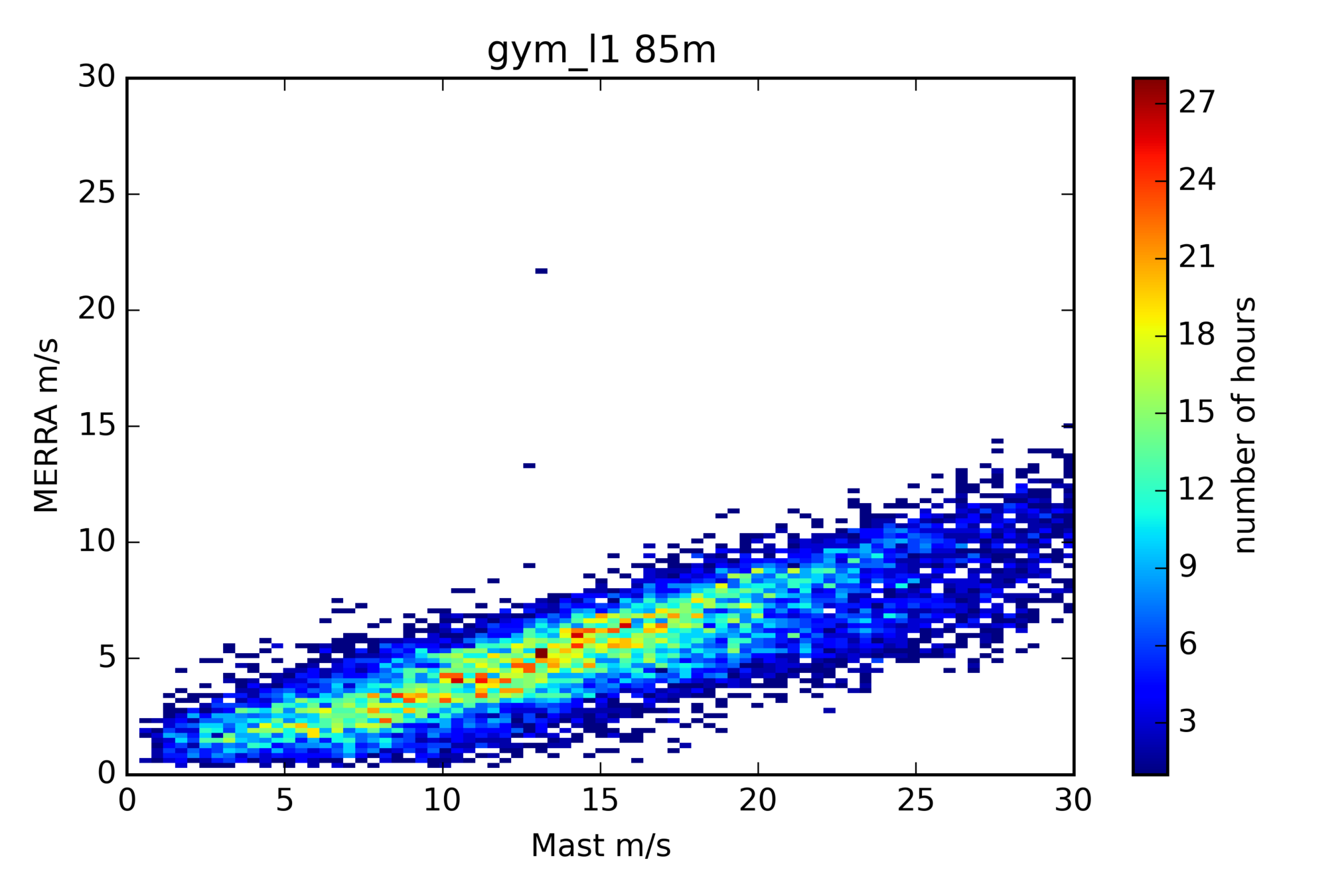
• This stage of the model can be evaluated by comparing timeseries to met masts
• Some sites better than other - higher degree of accuracy where all close points have similar surface conditions

ESTIMO_wind - RESTLESS wind simulation

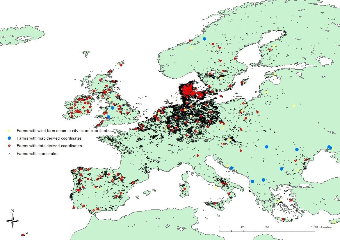
• All wind farms simulated separately using data from the windpower.net
• Site specific wind speed heights and farm curves
• Increased detail necessitates the use of Legion - great when it works ...

ESTIMO_wind - RESTLESS wind simulation

• The use of MERRA, including multiple wind speed heights, combined with site specific simulation and metadata significantly improves the accuracy of historic simulation
• Evaluating simulated wind generation is relatively straightforward due to good information on capacity and generation
• Countries with large diverse capacity are easier to simulate, as demonstrated by the plots of simualted vs measure German and UK wind 

ESTIMO_wind - RESTLESS wind simulation

• Location specific simualtion or countries wiht less spatial diversity are less easy to simulate and verfiy, as demonstrated by the plot of a single UK wind farm and Finland.

ESTIMO_wind - RESTLESS wind simulation

• Scenario modelling using European data can be more sophisticated than SpWIND due to more data
  • e.g. data on different classifications of wind farm as shown in the plots
• Scenarios first use operational, then under construction, approved and planned
  • Therefore representative of evolving capacity.
• Overall the RESTLESS method significantly improves accuracy and capability of Energy Space Time wind simulation
  • The maintained MERRA database also enables significant other work

Method improvements

Factors not incorporated in model

• Wake Effects
• Downtime
• Lag in turbine operation
• Energy Density over blades
• Air density
• Decline in performance with age
• Wind speed changes < 1 hour in frequency Location specific turbine curves
• Operating efficiency
• Atmospheric stability, surface roughness and orography in height correction

• Despite the considerable work and excellent data there is still a lot of room for improvement in the simulation, mainly down to the factors described to the right
• Some of this can be theoretically incorporated through statistcial alterations of the curves, as seen on the right
• Or better calibration, though this is not trivial
• Improved wind speed data can also be introduced in future studies
• Particularly in regional studies or those addressing climate change.

Solar generation

MERRA driven, gridded, global capacity factor timeseries derivation

• Like wind, methods for simulating solar generation are well established
• Even better, some of the are already coded in Python.
• For that reason Stefan Pfenningers GSEE model was used for PV generation estimation in RESTLESS, as described in the plot
• It was adapted slightly to run for all MERRA grid points for all hours
• Assuming a 1 MW fixed panel with optimum direction and tilt
• 207, 937 points  * 8760 hours * 37 years
  • > 67 billion generation values

*legion required again

• Evaluation and calibration of a solar simulation model is harder to carry out than wind, due to limited information on installed capacity and uncertain measured generation timeseries
• The meteorology is much simpler, however, therefore if some confidence can be gained in the simulation scenario modelling means simply multiplying capacity factors by assumed future capacities
• Climate change is unlikely to effect irradiance as much as wind speed over larger spatial scopes.

Methods for evaluating accuracy and variability

• Mean Absolute Deviation  (MAD)– using the in built pandas method .mad(), which does not totally agree with the manual method. A higher number describes larger deviation around the mean (or median) value.
• Un biased Variance (Var) - using the in built pandas method .cov(). See Covariance description below.
• Standard Deviation (StD) - using the in built pandas method .std(). A measure of dispersion around the mean. Low standard deviation indicates values are close to the mean.
• Mean -  using the in built pandas method .std(). Indicates average value of timeseries.    
• Pearson’s Correlation Coefficient (P) - using the in built pandas method .corr(). unbiased variance. 1 equals perfect positive correlation. Correlation is a normalised version of Covariance (therefore between 1 and -1) which allows comparison of different variables.
• Kendall’s Tau Correlation Coefficient (KTau) - using the in built pandas method .corr(). unbiased variance
• R2 correlation coefficient (R2) – using scipy.stats.linregress(x, y) - 1 equals perfect positive correlation
• Root Mean Squared Error (RMSE m/s) – using a formula. Average difference between timeseries.
• Covariance (COV) - using the in built pandas method .cov() the same measure as variance, but between timeseries. pairwise covariance. Covariance is a numerical measure that indicates the inter-dependency between two variables. A covariance of 0 indicates that the variables are totally independent. while a high and positive covariance value means that a variable is big when the other is big.

Case Study - Simulating wind and solar generation in South Korea

• Jupyter Notebook