Differentiable Programming
and its applications in Astro
20th Heidelberg Summer School
SEpt. 2025
François Lanusse
Université Paris-Saclay, Université Paris Cité, CEA, CNRS, AIM

The Pillars of Modern Deep Learning
The success of Deep Learning over the last ~10 years has relied on several factors:
- Availability of large amounts of data
-
Large amounts of compute
- Compute optimized for linear algebra
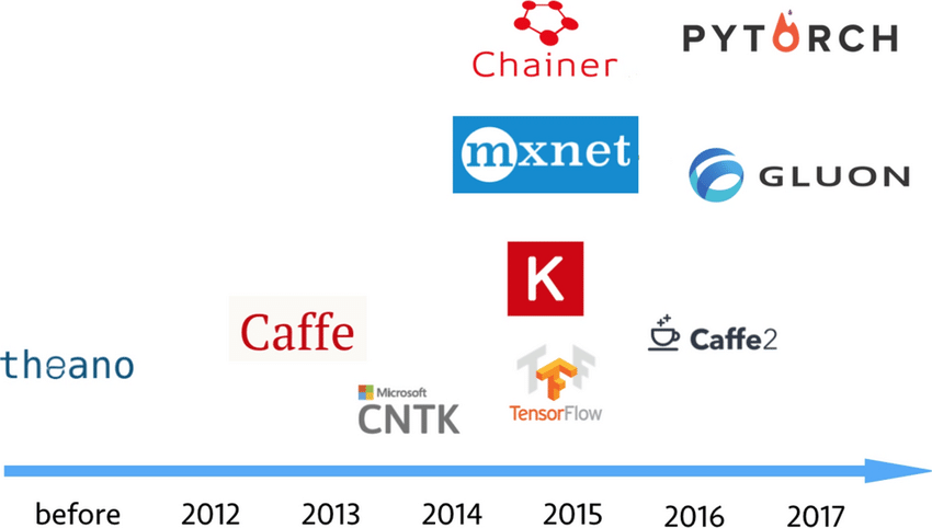
- Software frameworks that have enabled easy development and training of neural networks
The goal of this lecture is to steal reuse software and computational tools for Physics
Example of Differentiable Physics Models:
Jax-cosmo (Campagne et al. 2023)
Example of Differentiable Physics Model
FlowPM (Modi et al. 2021)


Initial conditions of
cosmological simulation
Reconstructed initial conditions
Reconstructed late-time density field
Data being fitted
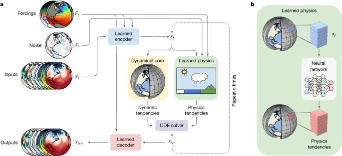
Examples of Differentiable Physics Models:
NeuralCGM (Kochkov et al. 2024)
What to expect from this lecture?
-
Learning objectives
- Understanding theoretical basis for automatic differentiation
- How to write differentiable programs in practice with JAX
- How to use differentiablity to enable optimization and Bayesian inference over physical models
-
Example use cases
- Solving pixel-level inverse problems in astronomical imaging
- Performing cosmological inference over a cosmological nbody simulation
A Short Primer on Automatic Differentiation
Mathematical definitions: Derivatives
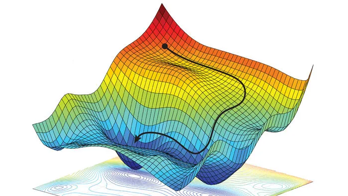
Gradient
- The gradient of a multivariate scalar function \( f : \mathbb{R}^n \rightarrow \mathbb{R}\) is:
- The gradient gives us the direction of
steepest ascent/descent
Typically, for a neural network defined by \( f(\mathbf{\theta}, \mathbf{x}) \) and a loss function \( \mathcal{L} \) we need to evaluate the gradient of the loss function with respect to parameters \( \mathbf{\theta} \): \( \nabla_{\mathbf{\theta}} \mathcal{L}(\theta, \mathbf{x}, \mathbf{y} ) \)
Jacobian
- The Jacobian of a function \( f : \mathbb{R}^n \rightarrow \mathbb{R}^m\) is:
How can we apply these mathematical notions to computer programs (i.e. your Python code)?

Finite differences (this is not AD)
- The simplest approach is
finite differences
for \( h \in \mathbb{R}^{+ *} \) sufficiently small
This approach induces 2 types of errors:
-
Truncation errors
The finite difference can be seen as truncating the Taylor expansion of \( f \)
$$ \frac{f(f + h) - f(x)}{h} = \frac{\partial f(x)}{\partial x} + o(h)$$ -
Round-off errors
Numerical error in computing \( f(x+h) - f(x) \) due to limited machine precision
- Central differences formula
Truncation error
Roundoff error
- A note on the computational cost of finite differences for a function \(f: \mathbb{R}^{n} \rightarrow \mathbb{R}^m \)
- Computational cost scale with the input dimension, insensitive to output dimension
- If we wanted to estimate the gradient for a 50M parameter resnet this way, we would need to compute the neural network function 50 million times!
- Computational cost scale with the input dimension, insensitive to output dimension
| Method | Error rate | Function calls for gradient |
|---|---|---|
| Forward/backward difference | o(h) | n + 1 |
| Central difference | o(h^2) | 2 n |
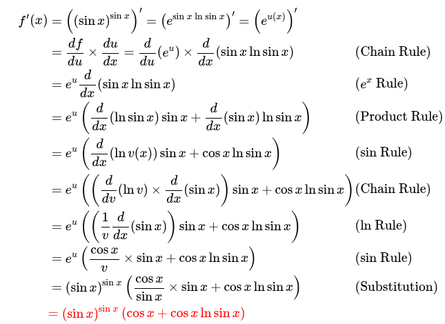
Symbolic Differentiation (still not AD)
- Programs like Mathematica or sympy can allow you to manipulate a symbolic expression and take its derivative using mathematical rules (e.g. chain rule)
from sympy import Symbol, sin, diff

x = Symbol('x')
f = (sin(x))**(sin(x))
derivative_f = diff(f, x)

print(f"The function is: {f}")
print(f"The derivative is: {derivative_f}")
The function is: sin(x)**sin(x)
The derivative is: (log(sin(x))*cos(x) + cos(x))*sin(x)**sin(x)- Unfortunately symbolic differentiation is not the panacea
-
Expression swell
- Control flow
-
Expression swell
def func(x):
  for i in range(4):
    x = 2*x**2 + 3*x + 1
  return x

f = func(x)
df = diff(f, x)def func(x):
if x > 2:
return x**2
else:
return x**3
try:
func(x)
except TypeError as err:
print("Error:", err)Error: cannot determine truth value of RelationalAutomatic Differentiation (yes, finally!)
- Let's start by the chain rule for 2 simple scalar functions:
Let \( f, g : \mathbb{R} \rightarrow \mathbb{R} \) and \( h = f \circ g \), then:
We need to compute 2 primitive derivatives and one intermediate value \( u\)- If we want to compute \(h(x)\) and \(h^\prime(x)\) this can algorithmically be done as:
- If we want to compute \(h(x)\) and \(h^\prime(x)\) this can algorithmically be done as:
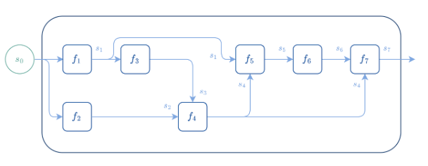
- Let us consider the more general case of \( k \) functions:
and define \( \mathbf{f} = \mathbf{f}_k \circ \ldots \circ \mathbf{f}_2 \circ \mathbf{f}_1: \mathbb{R}^n \rightarrow \mathbb{R}^m\)
- The chain rule can be applied to obtain the Jacobian of the entire computation
- Forming all the Jacobian matrices is impractical, but, it is easy to compute:
- columns: \( J_\mathbf{f} (\mathbf{x}) \mathbf{e}_i = \partial_i \mathbf{f} (\mathbf{x}) \), i.e. the i-th partial derivative of \( \mathbf{f} \)
- rows: \(\mathbf{e}_i^T J_\mathbf{f} (\mathbf{x}) = \nabla f_i (\mathbf{x})^T \), i.e. the gradient of the i-th dimension of \( \mathbf{f} \)
- Forming all the Jacobian matrices is impractical, but, it is easy to compute:
Reverse automatic differentiation (backprop)
- For wide matrices (m < n), it will be more efficient to build the rows of the Jacobian.
- This is typically the case for the loss function of a neural network (m = 1)
- This is typically the case for the loss function of a neural network (m = 1)
- This can be computed by recursively applying Vector Jacobian Products (VJP)
Forward pass
Backward pass
Forward pass
Backward pass
- Notes on reverse-mode automatic differentiation:
- It is necessary to store in memory all the intermediate steps of the forward pass (all \( \mathbf{x}_j \), typically called activations for neural networks).
- For a multivariate scalar function \( f: \mathbb{R}^n \rightarrow \mathbb{R} \), then \(e_i = [1] \) and the gradients with respect to all \( n \) parameters are obtained in one reverse pass, even for a network with billions of parameters.
Forward automatic differentiation
- For tall matrices (m > n), it will be more efficient to build the columns of the Jacobian.
- This can be computed by recursively applying Jacobian Vector Products (JVP)
Implementation of automatic differentiation
- To implement autodiff, we need the following:
- VJPs for primitive operations for reverse autodiff (and JVP for forward autodiff)
- A framework to keep track of the computational graph and intermediate activations
Luckily, we don't have to do it ourselves!


JAX: NumPy + Autograd + XLA
- JAX uses the NumPy API
=> You can copy/paste existing code, works pretty much out of the box
- JAX is a successor of autograd
=> You can transform any function to get forward or backward automatic derivatives (grad, jacobians, hessians, etc)
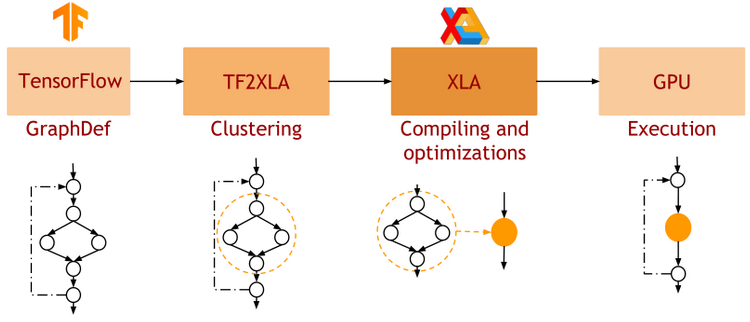
- JAX uses XLA as a backend
=> Same framework as used by TensorFlow (supports CPU, GPU, TPU execution)
import jax.numpy as np

m = np.eye(10) # Some matrix

def my_func(x):
  return m.dot(x).sum()

x = np.linspace(0,1,10)
y = my_func(x)
from jax import grad
df_dx = grad(my_func)
y = df_dx(x)
-
Pure functions
=> JAX is designed for functional programming: your code should be built around pure functions (no side effects)- Enables caching functions as XLA expressions
- Enables JAX's extremely powerful concept of composable function transformations
-
Just in Time (jit) Compilation
=> jax.jit() transformation will compile an entire function as XLA, which then runs in one go on GPU. -
Arbitrary order forward and backward autodiff
=> jax.grad() transformation will apply the d/dx operator to a function f -
Auto-vectorization
=> jax.vmap() transformation will add a batch dimension to the input/output of any function
def pure_fun(x):
  return 2 * x**2 + 3 * x + 2


def impure_fun_side_effect(x):
  print('I am a side effect')
  return 2 * x**2 + 3 * x + 2


C = 10. # A global variable
def impure_fun_uses_globals(x):
  return 2 * x**2 + 3 * x + C
# Decorator for jitting
@jax.jit
def my_fun(W, x):
return W.dot(x)
# or as an explicit transformation
my_fun_jitted = jax.jit(my_fun)def f(x):
return 2 * x**2 + 3 *x + 2
df_dx = jax.grad(f)
jac = jax.jacobian(f)
hess = jax.hessian(f)
# As decorator
@jax.vmap
def f(x):
  return 2 * x**2 + 3 *x + 2

# Can be composed
df_dx = jax.jit(jax.vmap(jax.grad(f)))
Let's try it out!
Practical Tutorial:
Solving Inverse Problems
With Explicit Physics Modeling
What are Linear Inverse Problems?


Deconvolution
Inpainting
Denoising
\( \mathbf{A} \) is known and encodes our physical understanding of the problem.
A motivating example: Image Deconvolution
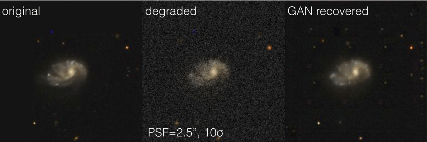
- The issue with black box deep learning inference
- No explicit control of noise, PSF, depth (needs to retrain if data changes)
- No guarantees physical properties will be preserved (e.g. flux)
- Robust uncertainty quantification is difficult

Some neural network \( f_{\theta} \)
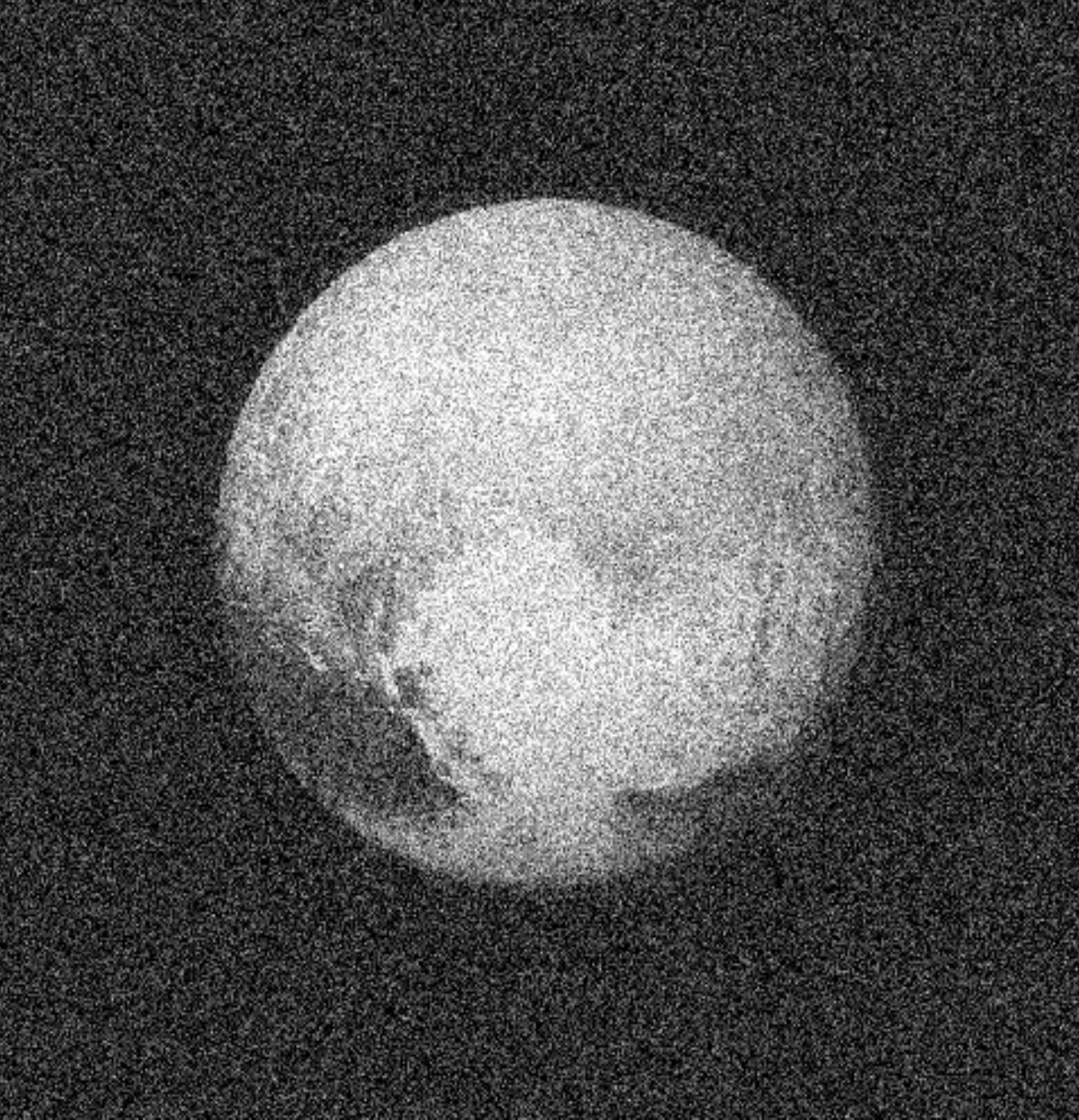
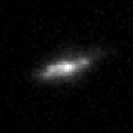
Hubble Space Telescope
Ground-Based Telescope
Example: GalaxyGAN (Schawinski et al. 2017)
A Bayesian view of the problem
- \( p(y|x) \) is the data likelihood, which contains the physics
- \( p(x) \) is our prior on the solution
With these concepts in hand, we can for instance estimate the Maximum A Posteriori solution:
Solving the MAP problem for deconvolution
Let's write down the difference pieces corresponding to our example deconvolution problem:
- Likelihood under a Gaussian noise model: $$ \log p(y | x) = -\frac{1}{2} \parallel y - \mathbf{P} \ast x \parallel_2^2 + cst $$ Where \( \mathbf{P} \) contains the instrumental response of the telescope, i.e. the PSF
- Prior under a very simple Gaussian model (spoiler alert: this will be too simple):
$$\log p(x) = - \lambda \parallel x \parallel_2^2 $$
=> Maximizing the log posterior requires differentiating through the instrument model! (PSF convolution)
We need a new tool to go probabilistic
import jax
import jax.numpy as jnp
from tensorflow_probability.substrates import jax as tfp
tfd = tfp.distributions

### Create a mixture of two scalar Gaussians:
gm = tfd.MixtureSameFamily(
  mixture_distribution=tfd.Categorical(
                 probs=[0.3, 0.7]),
  components_distribution=tfd.Normal(
                 loc=[-1., 1],
                 scale=[0.1, 0.5]))

# Evaluate probability
gm.log_prob(1.0)
Let's do it!
- Let's go to this notebook: https://tinyurl.com/diffprogtuto
Practical Tutorial:
Differentiable Particle-Mesh Simulation in JAX
Let's go to this notebook:
https://tinyurl.com/jaxpm
solution: https://tinyurl.com/jaxpm-solution
Practical Tutorial:
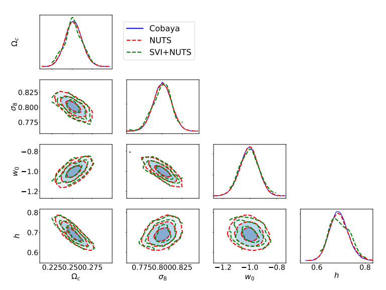
Probabilistic Inference with Differentiable Models
Let's build a Conditional Density Estimator with TFP
class MDN(nn.Module):
  num_components: int

  @nn.compact
  def __call__(self, x):
    x = nn.relu(nn.Dense(128)(x))
    x = nn.relu(nn.Dense(128)(x))
    x = nn.tanh(nn.Dense(64)(x))

    # Instead of regressing directly the value of the mass, the network
    # will now try to estimate the parameters of a mass distribution.
    categorical_logits = nn.Dense(self.num_components)(x)
    loc = nn.Dense(self.num_components)(x)
    scale = 1e-3 + nn.softplus(nn.Dense(self.num_components)(x))

    dist =tfd.MixtureSameFamily(
        mixture_distribution=tfd.Categorical(logits=categorical_logits),
        components_distribution=tfd.Normal(loc=loc, scale=scale))

    # To make it understand the batch dimension
    dist =  tfd.Independent(dist)

    # Returns a distribution !
    return dist
The core idea of Variational Inference is to assume a model distribution \( q_\phi \) and we fit it to the unknown posterior by minimizing the KL divergence:
$$ \mathbb{D}_{KL}\left( q_\phi(z) \parallel p(z | x) \right) = \mathbb{E}_{z \sim q_{\phi}} \left[ \log \frac{q_\phi(z)}{p(z | x)} \right] $$
$$ = \mathbb{E}_{z \sim q_{\phi}} \left[ \log q(z) \right] - \mathbb{E}_{z \sim q_{\phi}} \left[ \log p(z | x) \right] $$
$$ = \mathbb{E}_{z \sim q_{\phi}} \left[ \log q(z) \right] - \mathbb{E}_{z \sim q_{\phi}} \left[ \log p(x | z) + \log p(z) - \log p(x)\right] $$
$$ = \underbrace{\mathbb{D}_{KL}\left( q_\phi(z) \parallel p(z) \right) - \mathbb{E}_{z \sim q_{\phi}} \left[ \log p(x | z) \right]}_{{ELBO}} + \log p(x) $$
References
- Tutorials and Lectures
- Book