Cosmological Parameter Estimation Under Constrained Simulation Budget with
Optimal Transport-based Data Augmentation
Francois Lanusse on behalf of the Transatlantic Dream Team:
Noe Dia (Ciela), Sacha Guerrini (CosmoStat), Wassim Kabalan (CosmoStat/APC), Francois Lanusse (CosmoStat),
Julia Linhart (NYU), Laurence Perreault-Levasseur (Ciela), Benjamin Remy (SkAI), Sammy Sharief (Ciela),
Andreas Tersenov (CosmoStat), Justine Zeghal (Ciela)


Meet The Team!


Francois Lanusse
Sacha Guerrini
Benjamin Remy
Justine Zeghal
Julia Linhart
Sammy Sharief
Laurence
Perreault-Levasseur
Andreas Tersenov
Wassim Kabalan
Noé Dia
- Identifying the real challenge: very limited training data
- Not only do we only have 101 cosmologies, but we only have O(200) independent initial conditions.
- This is not an Uncertainty Quantification Challenge, it's a Data Efficient Deep Learning Challenge.
Guiding Principles for our Solution
3 different cosmologies,
at same systematics index
-
1st Principle: Choose a small convolutional architecture, don't spend a ton of time optimizing it.
-
2nd Principle: Don't do anything clever for the loss function, directly optimize the challenge metric.
-
3rd Principle: Think of the training set as finetuning/calibration data, pretrain the network on inexpensive emulated maps.
- This is a very relevant idea for actual cosmological inference where simulation data is expensive.
Identifying the real challenge: very limited training data
- Not only do we only have 101 cosmologies, but we only have O(200) independent initial conditions.
- This is not an Uncertainty Quantification Challenge, it's a Data Efficient Deep Learning Challenge.
Guiding Principles for our Solution
3 different cosmologies,
at same systematics index
1st Principle: Choose a small convolutional architecture, don't spend a ton of time optimizing it.
2nd Principle: Don't do anything clever for the loss function, directly optimize the challenge metric.
3rd Principle: Think of the training set as finetuning/calibration data, pretrain the network on inexpensive emulated maps.
- This is a very relevant idea for actual cosmological inference where simulating data is expensive.
Parameter Efficient Neural Architecture
EfficientNetV2 (Tan & Le 2021)
- Designed to optimize both training speed and accuracy
- 6.8x fewer parameters than ResNet → less overfitting risk
Early layers:
- Fused-MBConv blocks
- Regular 3x3 convolutions → get large feature maps quickly
Late layers:
- MBConv blocks
- Expands features → processes with lightweight depthwise convolutions → compressed featured
- Adds "squeeze-excitation" (SE) → learns which features are important
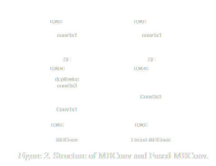
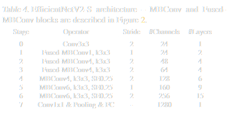
Tan & Le, EfficientNetV2: Smaller Models and Faster Training, ICML 2021
Training strategy
With only 20K samples, we overfit quickly. We therefore augmented the dataset with additional simulations.
Maximizing the challenge score:
Reshaping: remove most of the masked pixels
Data augmentation: rotations, flips, rollings


EfficientNetV2
Backbone
MLP
head
Embedding
Reshaping
Parameter Efficient Neural Architecture
Parameter Efficient Neural Architecture

Parameter Efficient Neural Architecture
EfficientNetV2
Backbone
MLP
head
Embedding
Parameter Efficient Neural Architecture
EfficientNetV2
Backbone
MLP
head
Embedding
EfficientNetV2 (Tan & Le 2021)
- designed to optimize both training speed and accuracy
- 6.8x fewer parameters than ResNet → less overfitting risk
Early layers:
- Fused-MBConv blocks
- regular 3x3 convolutions → get large feature maps quickly
Late layers:
- MBConv blocks
- Expands features → processes with lightweight depthwise convolutions → compressed featured
- Adds "squeeze-excitation" (SE) → learns which features are important
Parameter Efficient Neural Architecture
EfficientNetV2
Backbone
MLP
head
Embedding
Maximizing the score:
Parameter Efficient Neural Architecture
EfficientNetV2
Backbone
MLP
head
Embedding
Maximizing the score:
Reshaping: remove most of the masked pixels
Reshaping

Parameter Efficient Neural Architecture
EfficientNetV2
Backbone
MLP
head
Embedding
Maximizing the score:
Reshaping: remove most of the masked pixels
Reshaping
Augmentation
Data augmentation: rotations, flips, rollings
Parameter Efficient Neural Architecture
EfficientNetV2
Backbone
MLP
head
Embedding
Maximizing the score:
With only 20K samples, we overfit quickly. We therefore augmented the dataset with additional simulations.
Reshaping: remove most of the masked pixels
Data augmentation: rotations, flips, rollings
Augmentation
Reshaping
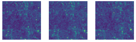
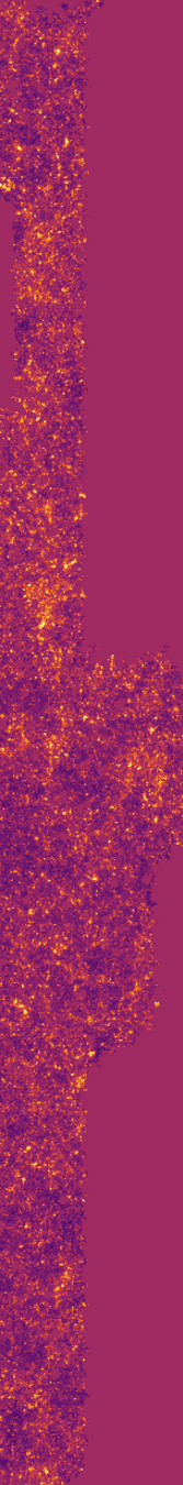
Fast LogNormal Simulations
Objective: Create cheap simulations close to the challenge's dataset.
Why model the matter field as LogNormal ?
- Positivity
- Enforce two-point statistics
- Easy to match the challenge simulation resolution
- Simple and fast to generate to create many LogNormal (~100 000) over a large range of cosmological parameters \( ( \Omega_m, S_8) \) and one nuisance parameter \( \Delta z \)
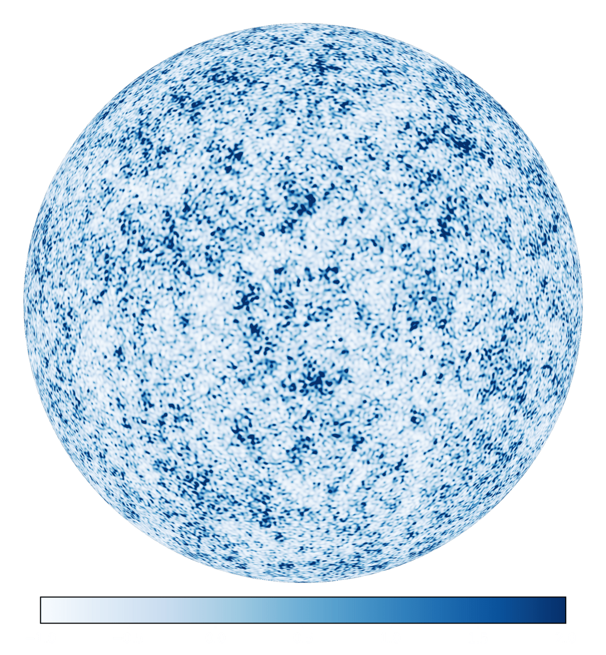
Kappa map obtained from the matter field using the GLASS package (Tessore et al., 2023).
→ Kappa map on the sphere
Fast LogNormal Simulations
LogNormal Convergence (patch)


Objective: Create cheap simulations close to the challenge's dataset.
Why model the matter field as LogNormal ?
- Positivity
- Enforce two-point statistics
- Easy to match the challenge simulation resolution
- Simple and fast to generate to create many LogNormal (~100 000) over a large range of cosmological parameters \( ( \Omega_m, S_8) \) and one nuisance parameter \( \Delta z \)
Kappa map obtained from the matter field using the GLASS package (Tessore et al., 2023).
→ Kappa map on the sphere
Fast LogNormal Simulations
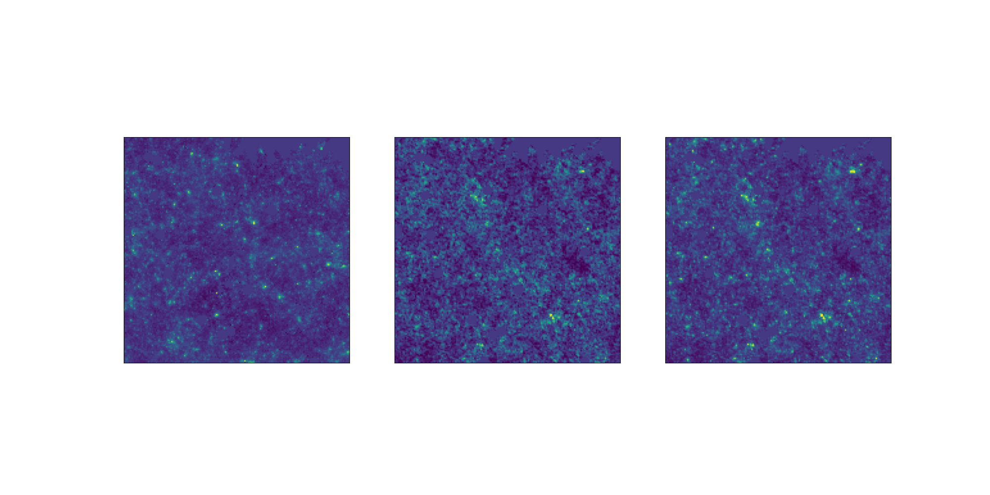
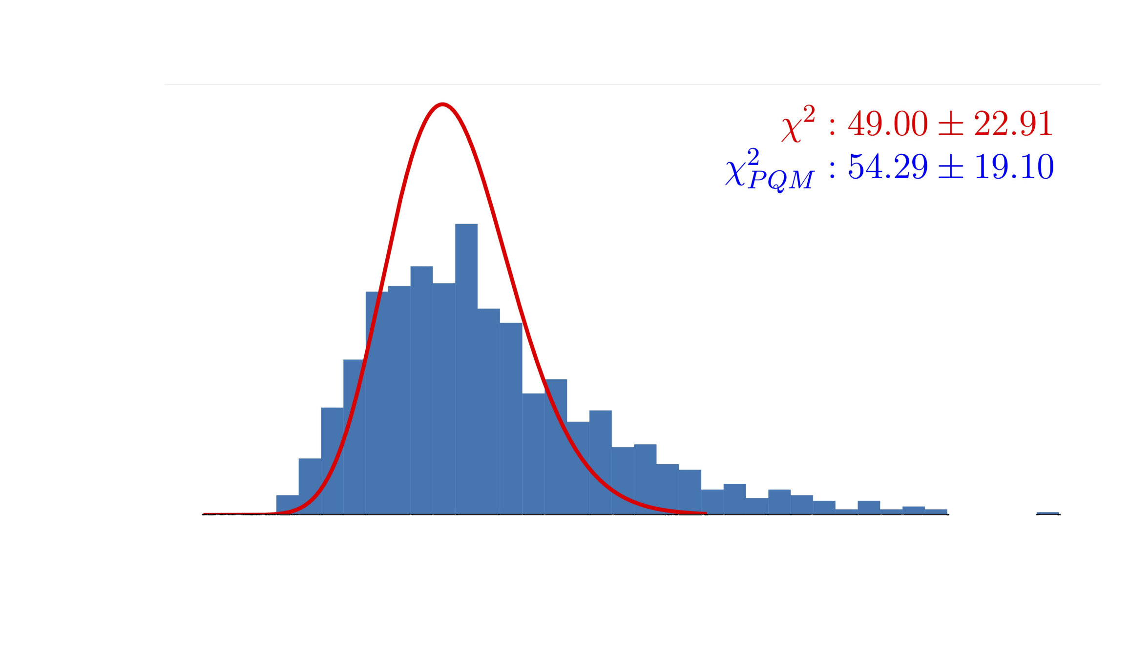
How good are the LogNormal simulations?
Comparison at same cosmology.
Challenge map
Power spectrum comparison
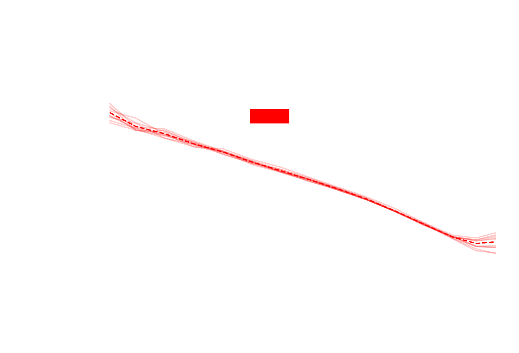
LogNormal map
Higher-order statistics
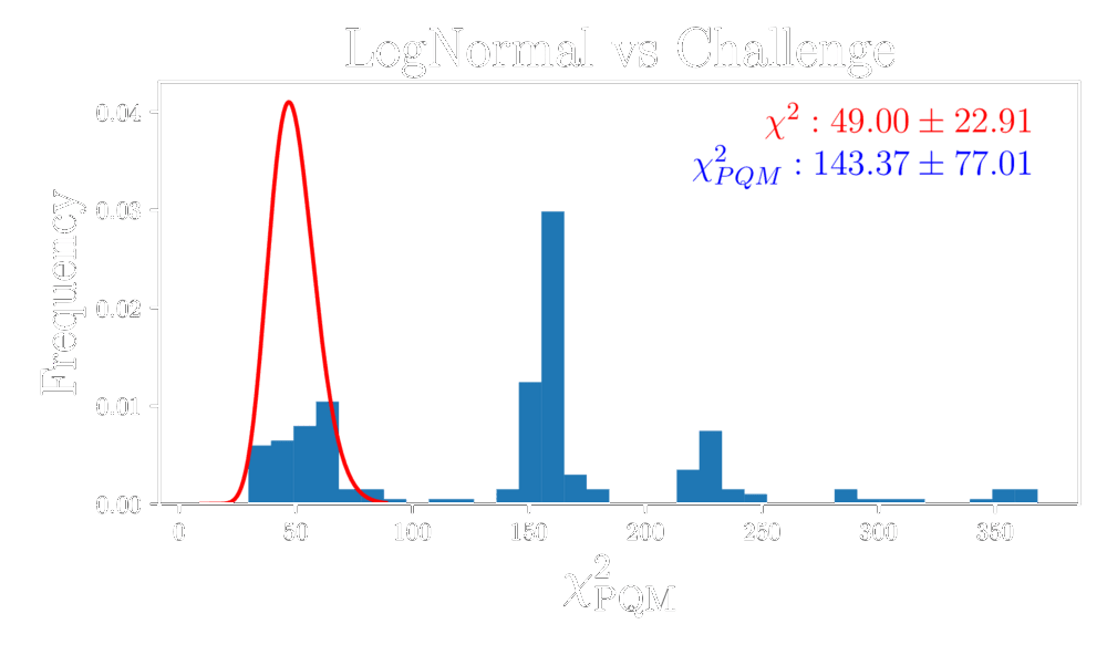
Data distribution comparison
Conditional Optimal Transport Adaptation
Conditional Optimal Transport Adaptation
LogNormal simulations are still very different.
Conditional Optimal Transport Adaptation
LogNormal simulations are still very different.
Objective: learning a pixel-level correction.
Conditional Optimal Transport Adaptation
LogNormal simulations are still very different.
Objective: learning a pixel-level correction.
Challenge like
LogNormal
Conditional Optimal Transport Adaptation
LogNormal simulations are still very different.
Objective: learning a pixel-level correction.
Problem: we do not have the initial conditions of the challenge simulations.
✅
❌
Challenge like
LogNormal
Challenge like
LogNormal
Conditional Optimal Transport Adaptation
LogNormal simulations are still very different.
Objective: learning a pixel-level correction.
Problem: we do not have the initial conditions of the challenge simulations.
Solution: Conditional Optimal Transport Flow-Matching (Kerrigan et al., 2024).
Where provides the pairs such that it minimizes the transport cost
Loss function:
Conditional Optimal Transport Adaptation
LogNormal simulations are still very different.
Objective: learning a pixel-level correction.
Problem: we do not have the initial conditions of the challenge simulations.
Solution: Conditional Optimal Transport Flow-Matching (Kerrigan et al., 2024).
- Transport any distributions
- Conditioned on Cosmology
- Unpaired datasets
Dataset 1
Dataset 2
Conditional Optimal Transport Adaptation
LogNormal simulations are still very different.
Objective: learning a pixel-level correction.
Problem: we do not have the initial conditions of the challenge simulations.
Solution: Conditional Optimal Transport Flow-Matching (Kerrigan et al., 2024).
- Transport any distributions
- Conditioned on Cosmology
- Unpaired datasets
Optimal
Transport Plan
Dataset 1
Dataset 2
Conditional Optimal Transport Adaptation
LogNormal simulations are still very different.
Objective: learning a pixel-level correction.
Problem: we do not have the initial conditions of the challenge simulations.
Solution: Conditional Optimal Transport Flow-Matching (Kerrigan et al., 2024).
- Transport any distributions
- Conditioned on Cosmology
- Unpaired datasets
- Learn the minimal transformation
- Zeghal et al., 2025 validated the kappa map emulation at the pixel level


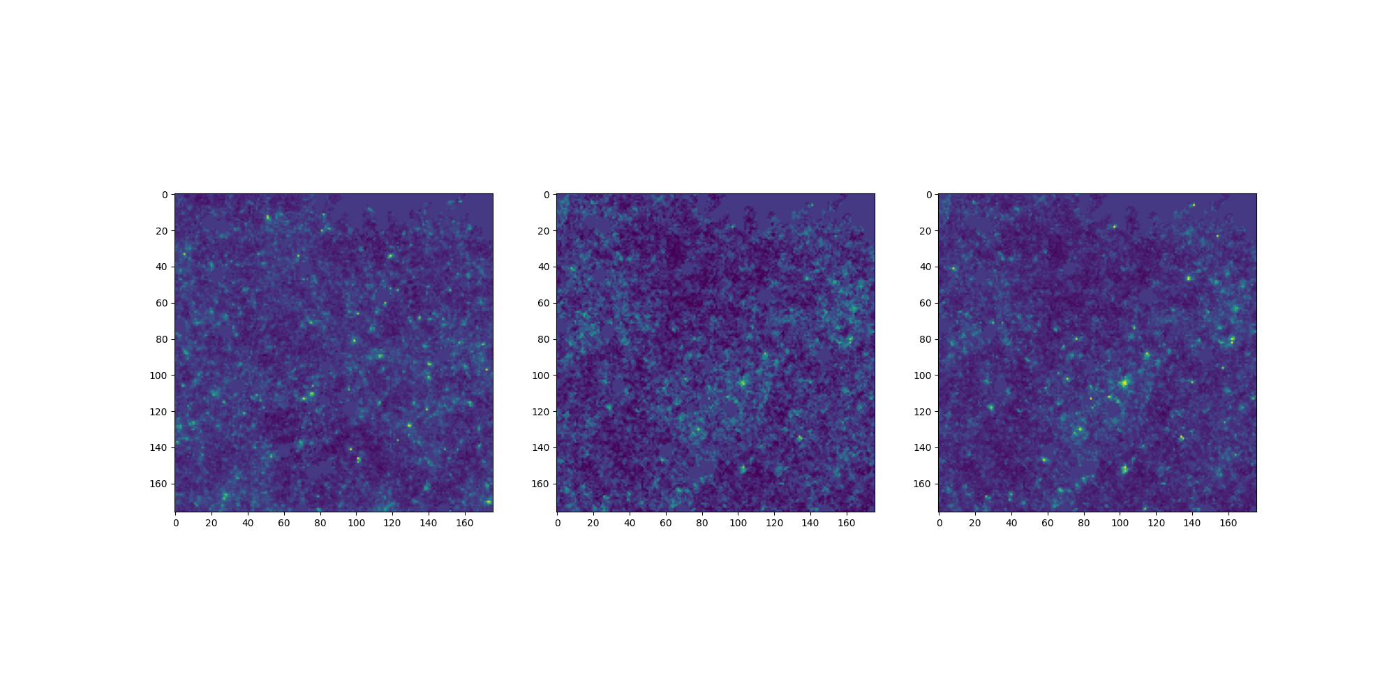
LogNormal
Emulated

Challenge simulation
VS
Conditional Optimal Transport Adaptation
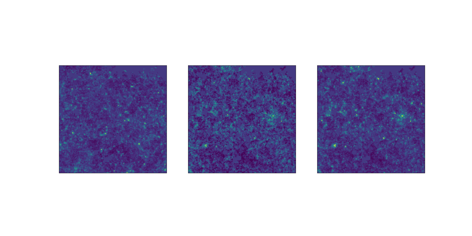
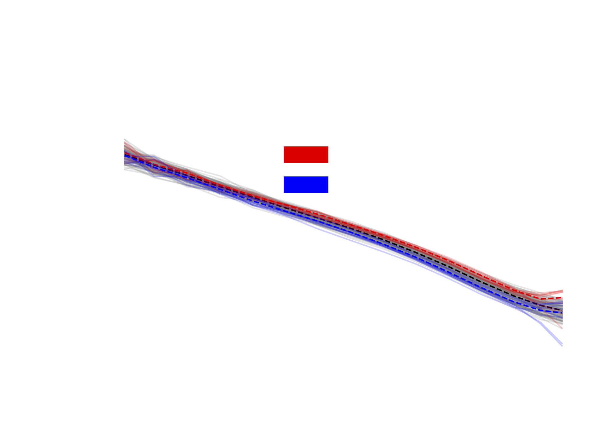
How good are the emulated simulations?
Comparison at same cosmology.
Challenge map
Power spectrum comparison
Emulated map
Higher-order statistics
Data distribution comparison
Progress and Results
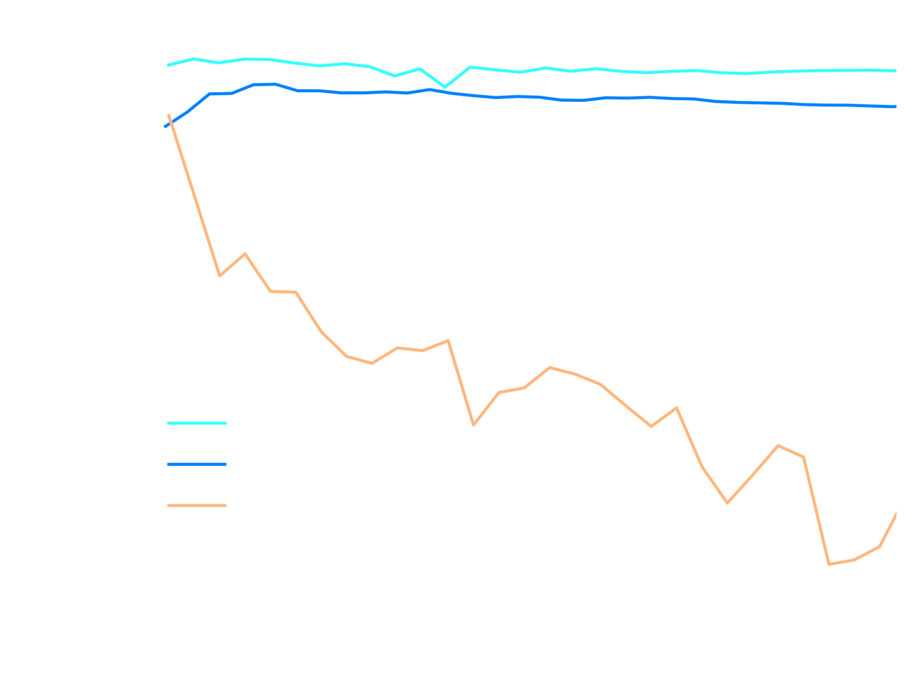
Validation score during pre-training
LR finetuning + early stopping
pre-training with OT maps
ensembling
pre-training with LogNormal maps
EfficientNetV2
| Score |
|---|
| 11.3856 |
| 11.5214 |
| 11.527 |
| 11.6468 |
| 11.6612 |
Summary of our progress
Takeaways
-
Data scarcity made UQ secondary to overfitting control.
With only 25k simulations over 101 cosmologies, the dominant practical problem was avoiding overfitting rather than exploring subtle properties of the posterior; most of the work went into regularization, augmentation, and careful validation splits.
-
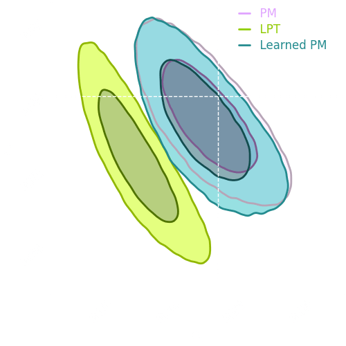
Lognormal + OT-based emulation is an effective way to augment training data.
Cheap LogNormal maps plus a pixel-level conditional optimal transport emulator gave a much better pretraining set than LogNormal alone and significantly improved generalization once you fine-tuned on the real challenge maps.
Conclusion: Even with a constrained simulation budget, you can get surprisingly strong end-to-end SBI performance by (i) exploiting cheap surrogate simulations for pretraining, and (ii) pushing “standard” supervised training (augmentations, regularization, careful design) much harder than is typical.
=> This suggests that practical SBI for real surveys may require fewer expensive simulations than one would naively assume.