|
|
Tutorial Neural Networks |
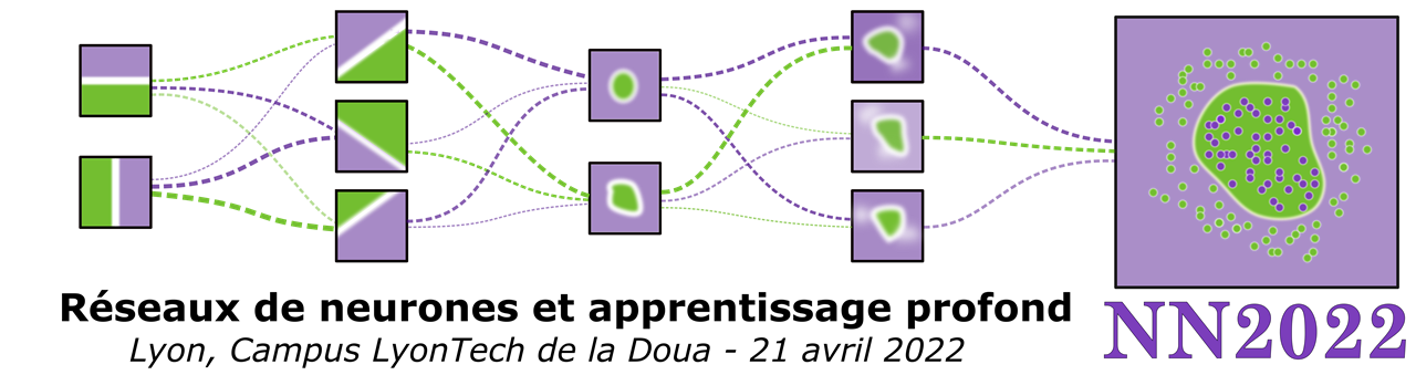

Emmanuel Roux, Rémi Emonet, Odyssée Merveille
CONTENT
- Introduction
- Data
- Model
- Method
- Conclusion
CONTENT
- Introduction
- Data
- Model
- Method
- Conclusion
- Examples of applications
- Historical background
- General pipeline
DALL-E-2
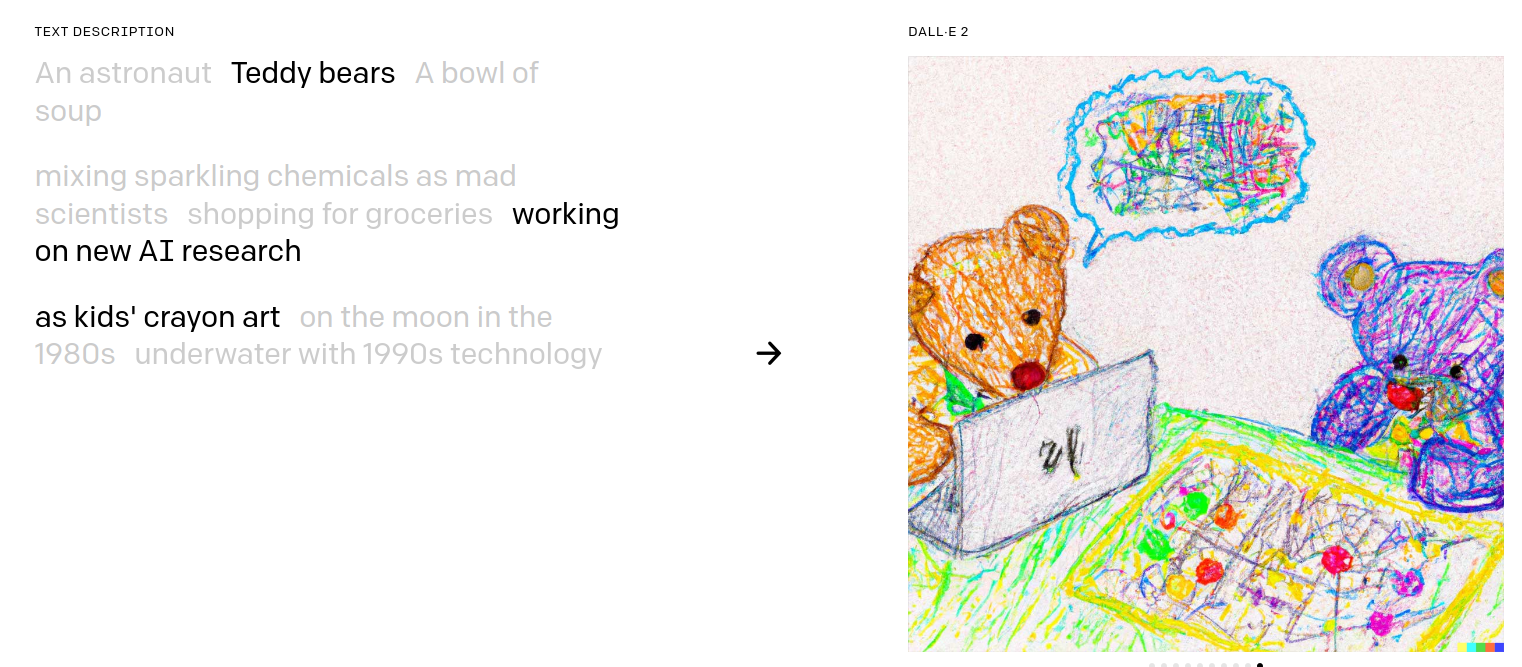
What do you think ?
- need of legal disclosure "AI generated synthetic media" ?
- metrics to evaluate possible harms and misuses ?
link to an article of the Stanford Institute for
Human-Centered Artificial Intelligence
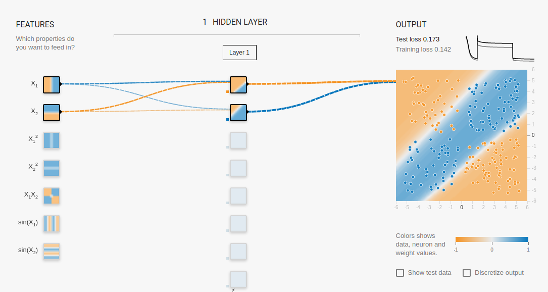
Natural Language Processing (NLP)
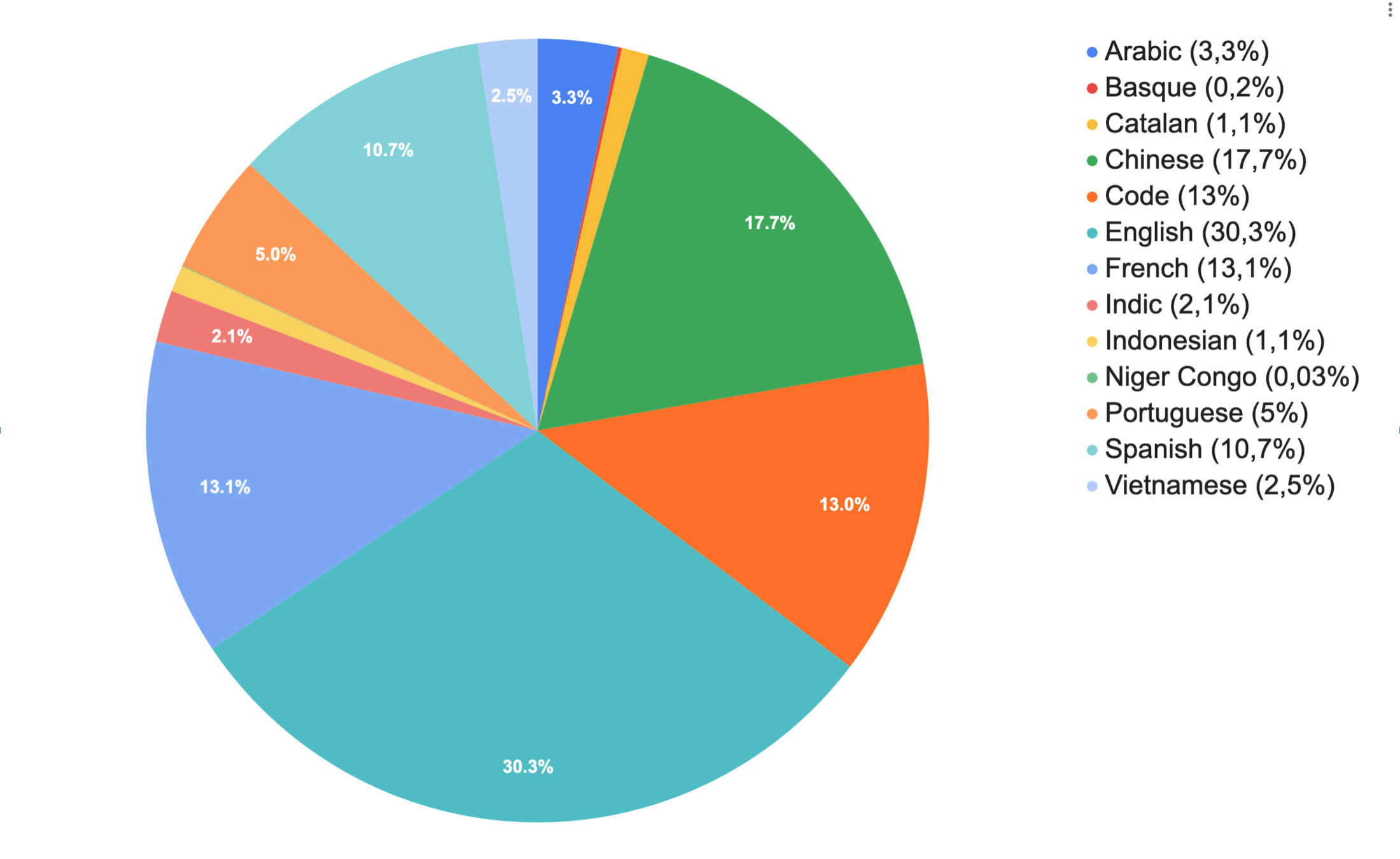
BigScience
46 different languages
176B parameters
training time: ~3-4 months
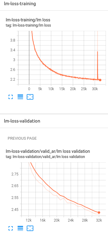

Link to Tensorboard
Ethical responsibility !
F. Urbina, F. Lentzos, C. Invernizzi, and S. Ekins, “Dual use of artificial-intelligence-powered drug discovery,” Nat Mach Intell, vol. 4, no. 3, Art. no. 3, Mar. 2022, doi: 10.1038/s42256-022-00465-9.
"We have spent decades using computers and AI to improve human health — not to degrade it. We were naive in thinking about the potential misuse of our trade, [...]."


Biochemical weapons design
On March, 4th 2022, the FTC, the U.S. agency in charge of consumer protection, ruled that an app developed by WW International (Kurbo app) did not respect data-collection laws :
collected data : age, gender, height, weight, and lifestyle choices.
children younger than 13 without permission from a parent
delete the data | destroy the models | $1.5 million fine

In 2021, the FTC made Everalbum destroy models that used images uploaded by users who hadn’t consented to face recognition
app vendors punished by the U.S. government for building algorithms based on illegally collected data
Better communication !

include cultural diversity in AI
sign langage recognition
link to the CVPR2021 challenge
Inclusive story teller
Better healthcare !
Personalized treatment (MRI)
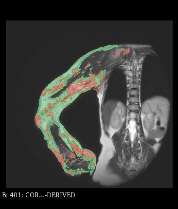
Stroke Prevention (TCD)
by Phd student Vindas Y.,
Medical Image Analysis, 2022, doi: 10.1016/j.media.2022.102437.
by PhD student Fraissenon A.
by PhD student Penarrubia L.
Medical physics, 2022,
doi: 10.1002/mp.15347.
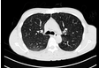
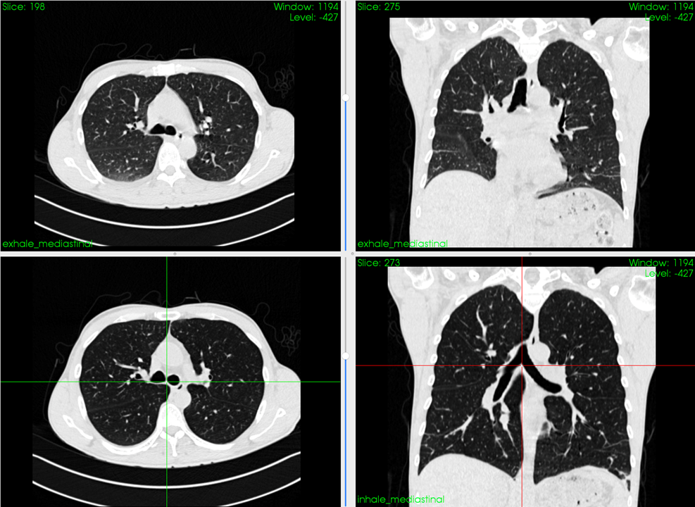
Ventilation imaging (CT)
classification tasks
Decision Boundary
regression tasks
binary
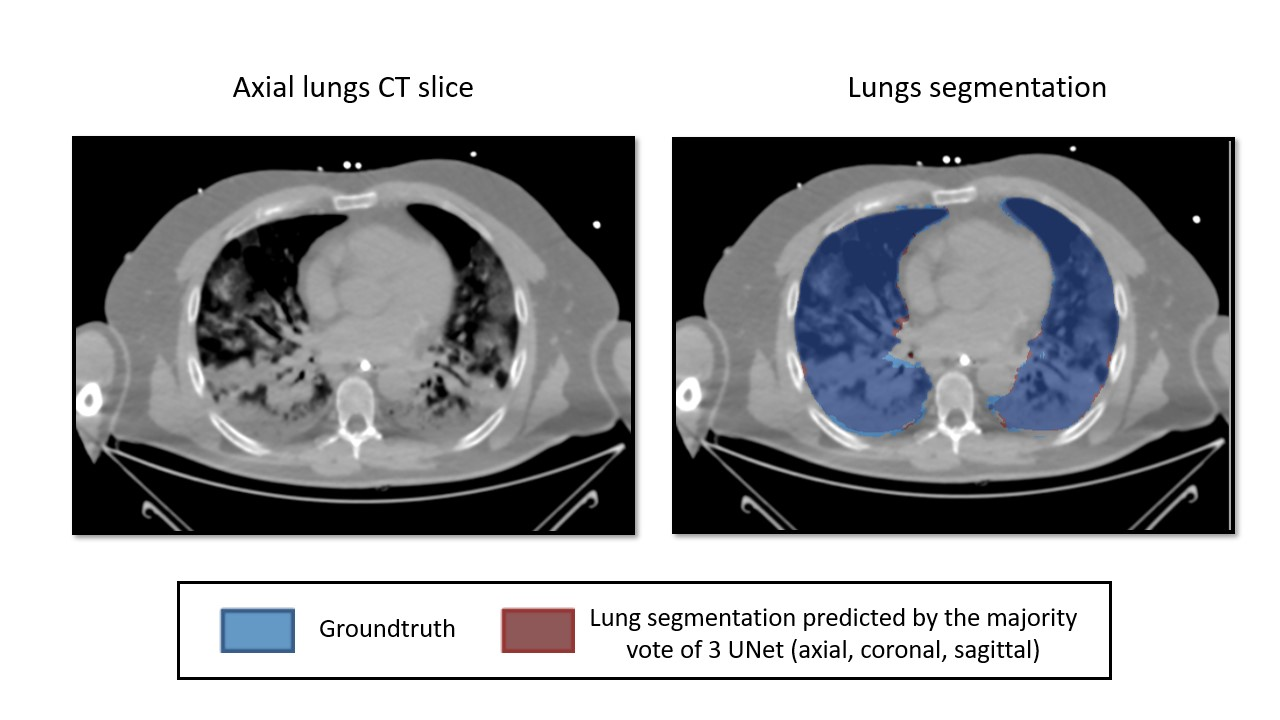
segmentation
multi-class
(multi-label)
predicted continuous value(s)
- Examples of applications
- Historical background
- General pipeline
- Introduction
- Data
- Model
- Method
- Conclusion
CONTENT
Machine Learning
Deep Learning
Artificial Intelligence
Inspired (and simplified) from the deeplearningbook.org
(I. Goodfellow and Y. Bengio, A. Courville, 2016)
historical background
Machine Learning
Deep Learning
Artificial Intelligence
Inspired from Sebastian Raschka's deep-learning course
historical background
Artificial Intelligence
Inspired from (Cardon D., Cointet J.-P., Mazieres A., 2018)
historical background
Artificial Intelligence
Inspired from (Cardon D., Cointet J.-P., Mazieres A., 2018)
DEDUCTIVE
rule-based
no need of examples
INDUCTIVE
example based
adaptation
Symbolic AI
connectionism
historical background
Cybernetics (40’s to 60’s)
Inspired from (Cardon D., Cointet J.-P., Mazieres A., 2018)
connexionism
Perceptron (Rosenblatt)
ADALINE (Widrow & Hoff)
(W. Ross Ashby)
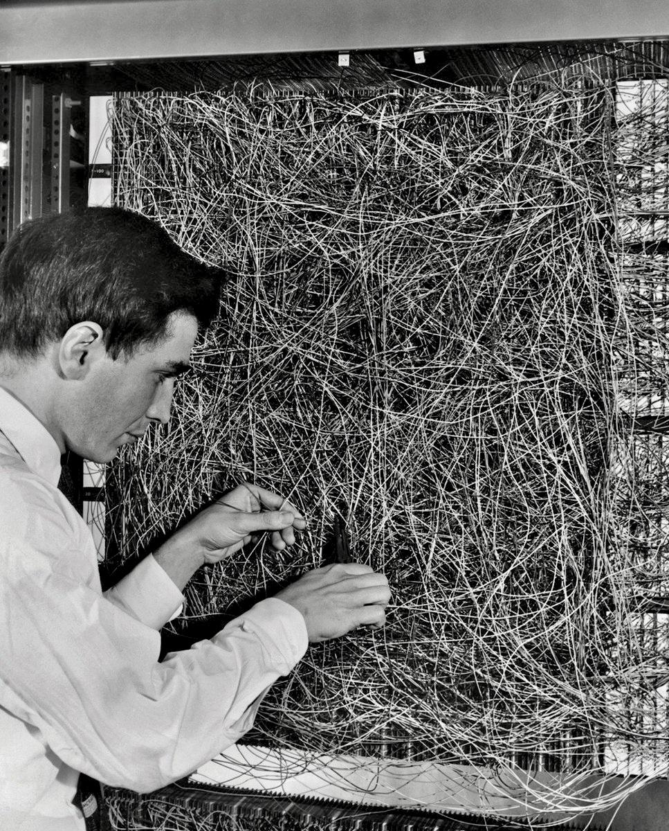
source wikipedia
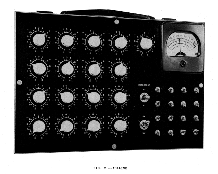
https://isl.stanford.edu/~widrow/papers/t1960anadaptive.pdf
historical background
Symbolic Artificial Intelligence (60’s to 80’s)
Inspired from (Cardon D., Cointet J.-P., Mazieres A., 2018)
Symbolic AI
MYCIN (Shortliffe): medical diagnoses (bacteria identification)
GUIDON (Clancey): teaching medical diagnostic strategy
CADUCEUS (Pople): internal medicine expert system
historical background
machine learning (00's to 10's)
deep learning (10's - now)
Image by Dake, Mysid
connexionism (80’s to 00’s)
historical background
- Examples of applications
- Historical background
- General pipeline
- Introduction
- Data
- Model
- Method
- Conclusion
CONTENT
data
General pipeline
sample
data
General pipeline
sample
data
General pipeline
sample
data
General pipeline
data
General pipeline
data
label
General pipeline
data
label
Dataset
General pipeline
data
Dataset
General pipeline
data
label
Dataset
General pipeline
neural network
data
label
Dataset
input
General pipeline
neural network
data
label
Dataset
output
General pipeline
neural network
data
label
Dataset
output
label
?
General pipeline
neural network
data
label
Dataset
loss function
General pipeline
neural network
data
label
General pipeline
Dataset
neural network
loss function
gradient
data
label
Dataset
loss function
update
General pipeline
neural network
gradient
data
label
Dataset
loss function
General pipeline
neural network
data
label
Dataset
loss function
General pipeline
neural network
data
label
Dataset
loss function
General pipeline
neural network
data
label
Dataset
loss function
General pipeline
neural network
data
label
Dataset
loss function
General pipeline
neural network
data
label
Dataset
loss function
General pipeline
neural network
data
label
Dataset
loss function
General pipeline
neural network
for data, label in dataloader:
    label_pred = model(data) # forward pass
    loss = (label - label_pred)**2 # loss
    loss.backward() # loss gradient
    optimizer.step() # model update
data
label
Dataset
loss function
General pipeline
neural network
for data, label in dataloader:
    label_pred = model(data) # forward pass
    loss = (label - label_pred)**2 # loss
    loss.backward() # loss gradient
    optimizer.step() # model update
data
label
Dataset
loss function
General pipeline
neural network
for data, label in dataloader:
    label_pred = model(data) # forward pass
    loss = (label - label_pred)**2 # loss
    loss.backward() # loss gradient
optimizer.step() # model updatedata
label
Dataset
loss function
General pipeline
neural network
for data, label in dataloader:
    label_pred = model(data) # forward pass
    loss = (label - label_pred)**2 # loss
    loss.backward() # loss gradient
optimizer.step() # model updategradient
data
label
Dataset
loss function
General pipeline
neural network
for data, label in dataloader:
    label_pred = model(data) # forward pass
    loss = (label - label_pred)**2 # loss
    loss.backward() # loss gradient
optimizer.step() # model updateupdate
gradient
loss function
General pipeline
neural network
for data, label in dataloader:
    label_pred = model(data) # forward pass
    loss = (label - label_pred)**2 # loss
    loss.backward() # loss gradient
    optimizer.step() # model update
data
label
Dataset
loss function
General pipeline
neural network
for data, label in dataloader:
    label_pred = model(data) # forward pass
    loss = (label - label_pred)**2 # loss
    loss.backward() # loss gradient
    optimizer.step() # model update
data
label
Dataset
loss function
General pipeline
neural network
for data, label in dataloader:
    label_pred = model(data) # forward pass
    loss = (label - label_pred)**2 # loss
    loss.backward() # loss gradient
    optimizer.step() # model update
data
label
Dataset
loss function
General pipeline
neural network
for data, label in dataloader:
    label_pred = model(data) # forward pass
    loss = (label - label_pred)**2 # loss
    loss.backward() # loss gradient
    optimizer.step() # model update
data
label
Dataset
loss function
General pipeline
neural network
for data, label in dataloader:
    label_pred = model(data) # forward pass
    loss = (label - label_pred)**2 # loss
    loss.backward() # loss gradient
    optimizer.step() # model update
data
label
Dataset
gradient
loss function
General pipeline
neural network
for data, label in dataloader:
    label_pred = model(data) # forward pass
    loss = (label - label_pred)**2 # loss
    loss.backward() # loss gradient
    optimizer.step() # model update
data
label
Dataset
update
gradient
loss function
General pipeline
neural network
for data, label in dataloader:
    label_pred = model(data) # forward pass
    loss = (label - label_pred)**2 # loss
    loss.backward() # loss gradient
    optimizer.step() # model update
data
label
Dataset
loss function
General pipeline
neural network
for data, label in dataloader:
    label_pred = model(data) # forward pass
    loss = (label - label_pred)**2 # loss
    loss.backward() # loss gradient
    optimizer.step() # model update
data
label
Dataset
loss function
General pipeline
neural network
for data, label in dataloader:
    label_pred = model(data) # forward pass
    loss = (label - label_pred)**2 # loss
    loss.backward() # loss gradient
    optimizer.step() # model update
data
label
Dataset
loss function
General pipeline
neural network
for data, label in dataloader:
    label_pred = model(data) # forward pass
    loss = (label - label_pred)**2 # loss
    loss.backward() # loss gradient
    optimizer.step() # model update
data
label
Dataset
loss function
General pipeline
neural network
for data, label in dataloader:
    label_pred = model(data) # forward pass
    loss = (label - label_pred)**2 # loss
    loss.backward() # loss gradient
    optimizer.step() # model update
data
label
Dataset
gradient
loss function
General pipeline
neural network
for data, label in dataloader:
    label_pred = model(data) # forward pass
    loss = (label - label_pred)**2 # loss
    loss.backward() # loss gradient
    optimizer.step() # model update
data
label
Dataset
gradient
update
General pipeline
neural network
data
label
Dataset
loss function
gradient
update
Model
Method
General pipeline
neural network
data
label
Dataset
loss function
gradient
update
Model
Method
- Introduction
- Data
- Model
- Method
- Conclusion
- Pre-processing
- Notations (2-D example)
CONTENT
data - pre-processing
- resampling
- feature scaling
- data augmentation
data - pre-processing
1. resampling
data - pre-processing
1. resampling
data - pre-processing
normalization
MinMax
2. feature scaling
standardisation
data - pre-processing
2. feature scaling
scale
crop (patches)
rotate
flip
perspectives ...
filtering/noise
data - pre-processing
3. data augmentation
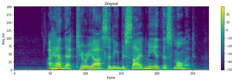
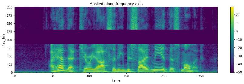
audio and time-frequency representations
data - pre-processing
3. data augmentation
audio and time-frequency representations
data - pre-processing
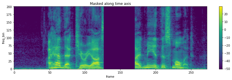
3. data augmentation
audio and time-frequency representations
data - pre-processing
time stretching
3. data augmentation
audio and time-frequency representations
data - pre-processing
time stretching
3. data augmentation
- Introduction
- Data
- Model
- Method
- Conclusion
- Pre-processing
- Notations (2-D example)
CONTENT
data
label
data - notations
data
label
sample
data - notations
data
label
sample
data - notations
2D points example
input space
data
label
and its label
sample
data - notations
2D points example
data
label
sample
data - notations
2D points example
data
label
sample
data - notations
2D points example
data
label
data - notations
2D points example
data
label
data - notations
2D points example
unknown distribution
data
label
data - notations
2D points example
new domain
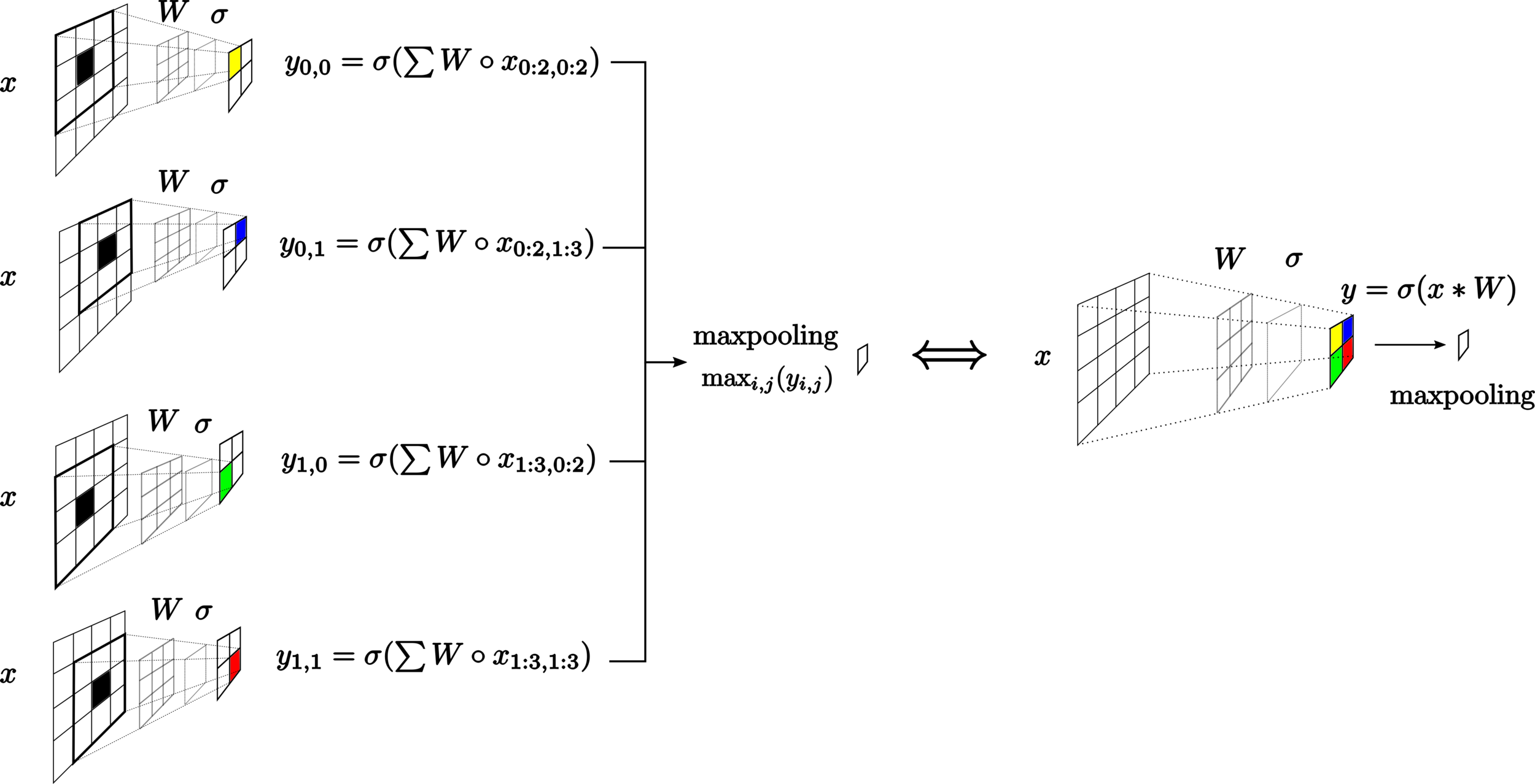
General pipeline
neural network
Dataset
loss function
gradient
update
Model
Method
data
label
- Introduction
- Data
- Model
- Method
- Conclusion
CONTENT
- Artificial Neuron
- Neural Network (NN)
- XOR (with CooLearning)
- Convolutions (CNN)
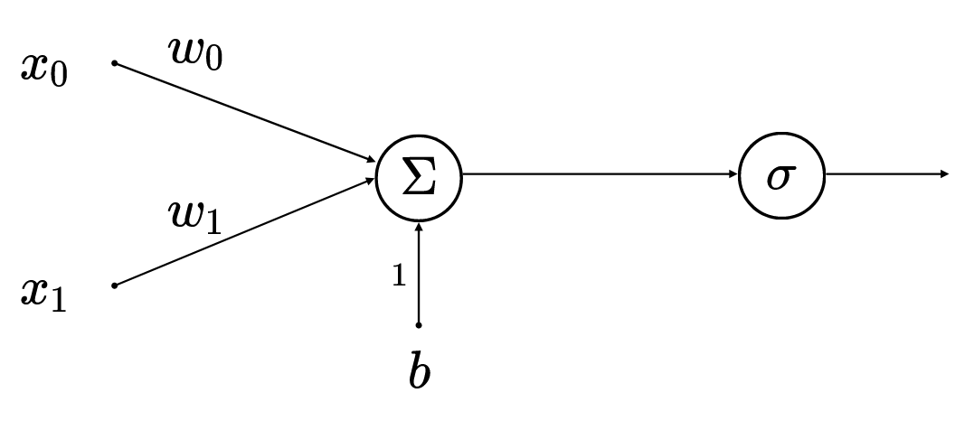
model - artifical neuron
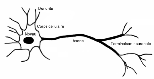
Input
Output
model - artifical neuron
model - artifical neuron
model - artifical neuron
model - artifical neuron
model - artifical neuron
model - artifical neuron
3 weights
1 biais
model - artifical neuron
model - artifical neuron
Activation function
Activation functions
model - artifical neuron
ReLU
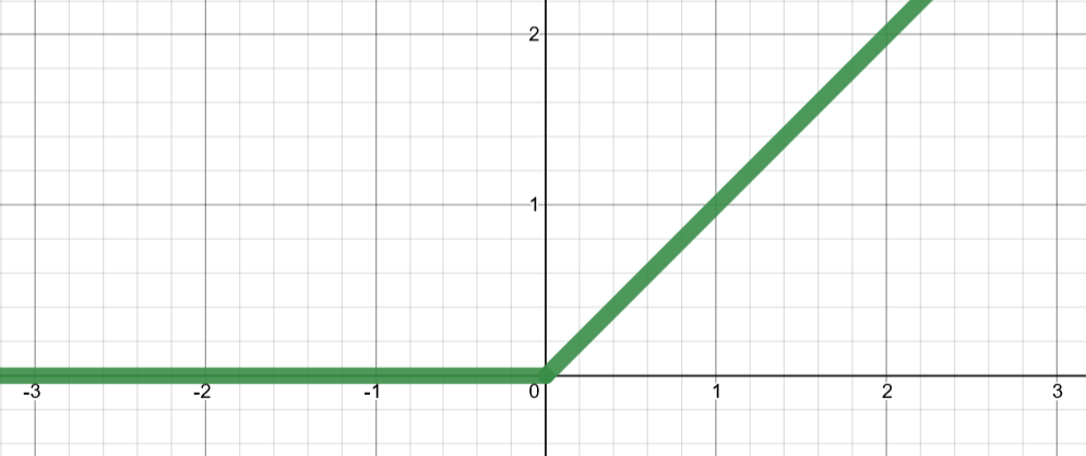
Activation functions
model - artifical neuron
tanh
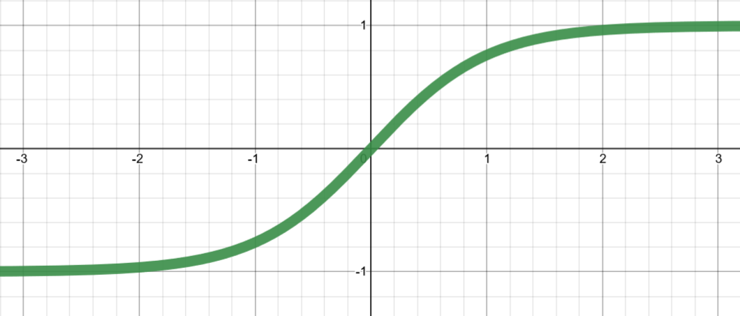
Activation functions
model - artifical neuron
Sigmoid (logistic)
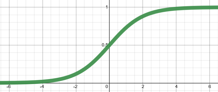
Activation functions
model - artifical neuron
Softmax
pseudo-probabilités
model - artifical neuron
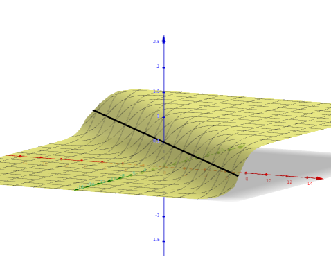
3-D interactive
visualization
Sigmoid (logistic)
2 inputs
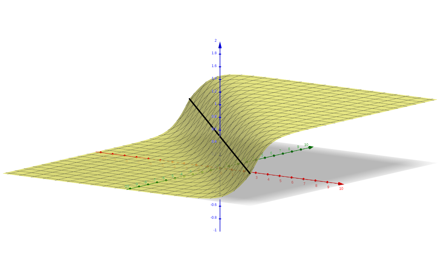
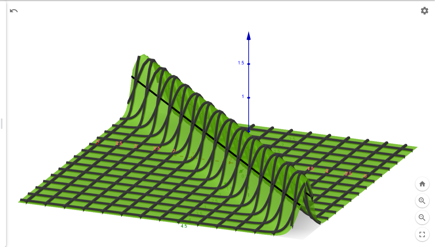
model - artifical neuron
2 inputs
model - artifical neuron
2 inputs
Sigmoid
2 inputs
model - artifical neuron
2 inputs
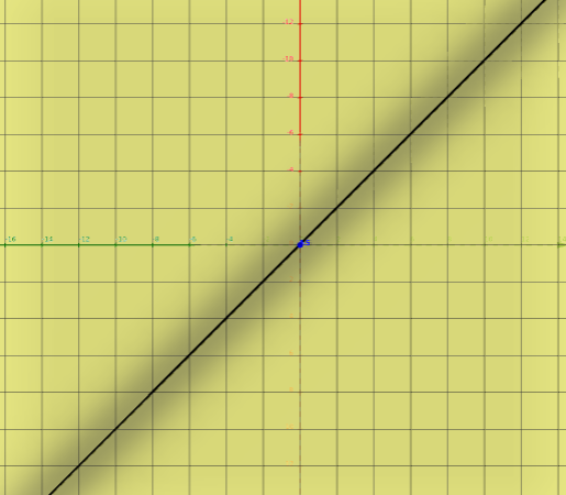
top view
2 inputs
model - artifical neuron
2 inputs
top view
- Introduction
- Data
- Model
- Method
- Conclusion
CONTENT
- Artificial Neuron
- Neural Network (NN)
- XOR (with CooLearning)
- Convolutions (CNN)
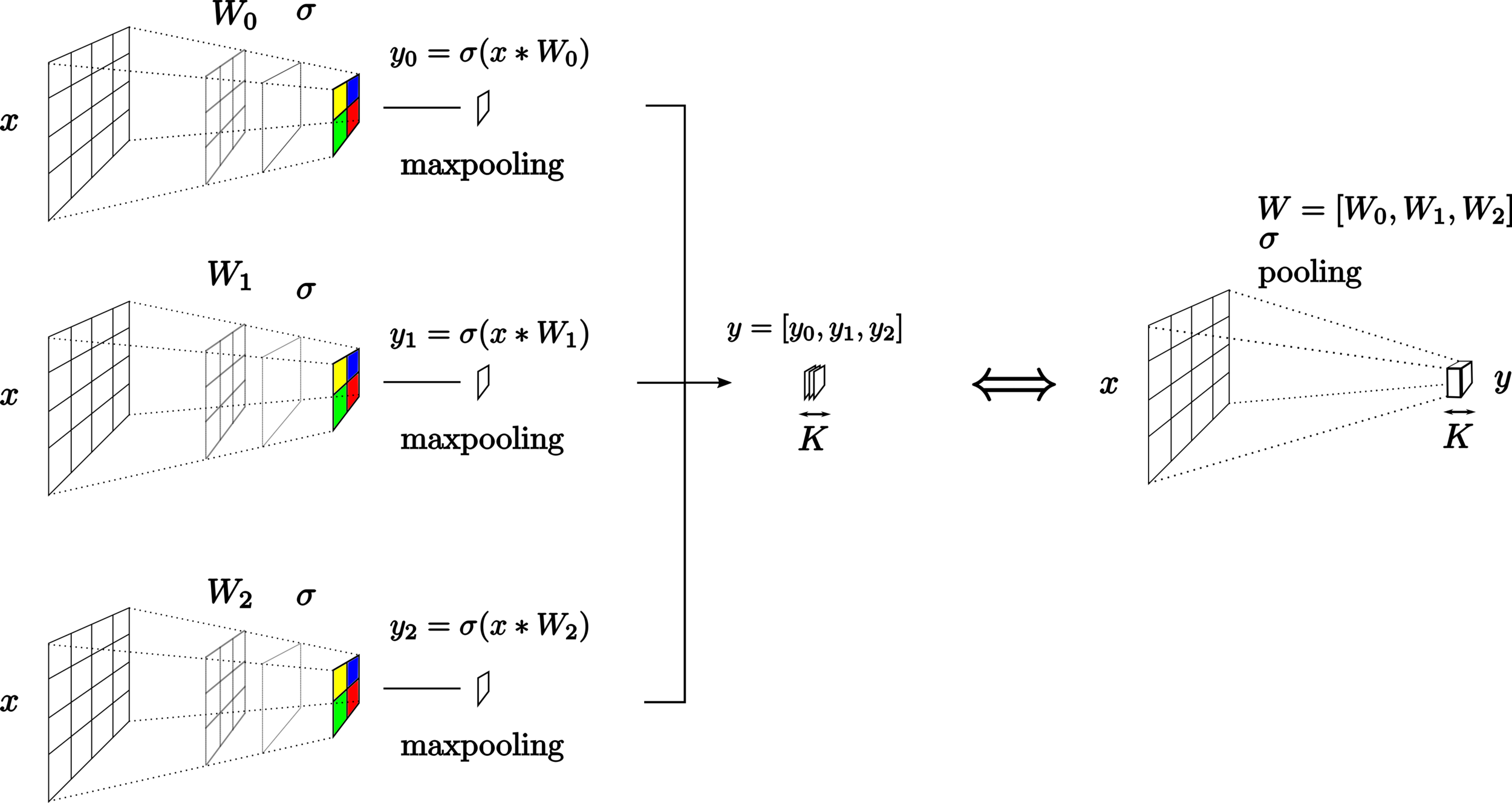
model - neural network
2-neurons input layer
model - neural network

2-neurons input layer
model - neural network
2-neurons input layer
1 neuron output layer
Perceptron
deep neural network
(MLP)
model - neural network
5-neurons input layer
1 neuron output layer
3-neurons hidden layer
model - neural network
deep neural network
(MLP)
5-neurons input layer
1 neuron output layer
3-neurons first
hidden layers
3-neurons second
hidden layers
model - neural network
deep neural network
(MLP)
12 neurons
BUT
64 parameters !
5x5 + 5 = 30
5x3 + 3 = 18
3x3 + 3 = 12
3x1 + 1 = 4
model - neural network
- Introduction
- Data
- Model
- Method
- Conclusion
CONTENT
- Artificial Neuron
- Neural Network (NN)
- XOR (with CooLearning)
- Convolutions (CNN)
model - neural network
model - neural network
- Introduction
- Data
- Model
- Method
- Conclusion
CONTENT
- Artificial Neuron
- Neural Network (NN)
- XOR (with CooLearning)
- Convolutions (CNN)
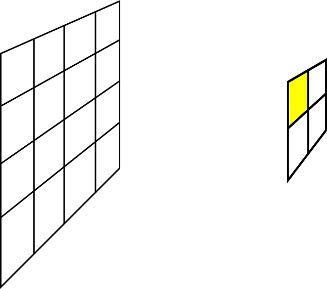
| 0 | 4 | 2 |
| 2 | 0 | 2 | 2 | 0 | 4 | 2 | 1 |
model - convolutions
| 0 | 4 | 2 |
| 2 | 0 | 2 | 2 | 0 | 4 | 2 | 1 |
model - convolutions
| 0 | 4 | 2 |
| 2 | 0 | 2 | 2 | 0 | 4 | 2 | 1 |
model - convolutions
| 0 | 4 | 2 |
| 2 | 0 | 2 | 2 | 0 | 4 | 2 | 1 |
model - convolutions
| 0 | 4 | 2 |
| 2 | 0 | 2 | 2 | 0 | 4 | 2 | 1 |
| 4 |
model - convolutions
| 0 | 4 | 2 |
| 2 | 0 | 2 | 2 | 0 | 4 | 2 | 1 |
| 4 |
model - convolutions
| 0 | 4 | 2 |
| 2 | 0 | 2 | 2 | 0 | 4 | 2 | 1 |
| 4 |
model - convolutions
| 0 | 4 | 2 |
| 2 | 0 | 2 | 2 | 0 | 4 | 2 | 1 |
| 4 | 12 |
model - convolutions
| 0 | 4 | 2 |
| 2 | 0 | 2 | 2 | 0 | 4 | 2 | 1 |
| 4 | 12 |
model - convolutions
| 0 | 4 | 2 |
| 2 | 0 | 2 | 2 | 0 | 4 | 2 | 1 |
| 4 | 12 |
model - convolutions
| 0 | 4 | 2 |
| 2 | 0 | 2 | 2 | 0 | 4 | 2 | 1 |
| 4 | 12 | 8 |
model - convolutions
| 0 | 4 | 2 |
| 2 | 0 | 2 | 2 | 0 | 4 | 2 | 1 |
| 4 | 12 | 8 |
model - convolutions
| 0 | 4 | 2 |
| 2 | 0 | 2 | 2 | 0 | 4 | 2 | 1 |
| 4 | 12 | 8 |
model - convolutions
| 0 | 4 | 2 |
| 2 | 0 | 2 | 2 | 0 | 4 | 2 | 1 |
| 4 | 12 | 8 | 8 |
model - convolutions
| 0 | 4 | 2 |
| 2 | 0 | 2 | 2 | 0 | 4 | 2 | 1 |
| 4 | 12 | 8 | 8 | 20 |
model - convolutions
| 0 | 4 | 2 |
| 2 | 0 | 2 | 2 | 0 | 4 | 2 | 1 |
| 4 | 12 | 8 | 8 | 20 | 10 |
model - convolutions
| 0 | 4 | 2 |
| 2 | 0 | 2 | 2 | 0 | 4 | 2 | 1 |
| 4 | 12 | 8 | 8 | 20 | 10 |
| 0 | 4 | 2 |
model - convolutions
| 0.2 | 0.5 | 0.3 | 0.3 | 0.9 | 0.4 |
| 0 | 4 | 2 |
| 2 | 0 | 2 | 2 | 0 | 4 | 2 | 1 |
| 4 | 12 | 8 | 8 | 20 | 10 |
| 0.2 | 0.5 | 0.3 | 0.3 | 0.9 | 0.4 |
| 0 | 4 | 2 |
| 0.5 | 0.3 | 0.9 |
model - convolutions
| 0 | 4 | 2 |
| 2 | 0 | 2 | 2 | 0 | 4 | 2 | 1 |
| 8 | 4 | 12 | 8 | 8 | 20 | 10 | 4 |
| 0 | 4 | 2 |
model - convolutions
(zero) padding
| 0 | 4 | 2 |
| 0 | 4 | 2 |
0
0
| 0 | 4 | 2 |
| 0 | 2 | 0 | 2 | 2 | 0 | 4 | 2 | 1 | 0 |
| 8 | 4 | 12 | 8 | 8 | 20 | 10 | 4 |
| 0 | 4 | 2 |
model - convolutions
STRIDE
| 0 | 4 | 2 |
| 0 | 2 | 0 | 2 | 2 | 0 | 4 | 2 | 1 | 0 |
| 8 | 4 | 12 | 8 | 8 | 20 | 10 | 4 |
| 0 | 4 | 2 |
model - convolutions
STRIDE
| 0 | 4 | 2 |
| 0 | 2 | 0 | 2 | 2 | 0 | 4 | 2 | 1 | 0 |
| 8 | 4 | 12 | 8 | 8 | 20 | 10 | 4 |
| 0 | 4 | 2 |
model - convolutions
STRIDE
| 0 | 4 | 2 |
| 0 | 2 | 0 | 2 | 2 | 0 | 4 | 2 | 1 | 0 |
| 8 | 4 | 12 | 8 | 8 | 20 | 10 | 4 |
| 0 | 4 | 2 |
model - convolutions
STRIDE
model - convolutions
2-D convolutions
model - convolutions

model - convolutions
model - convolutions
model - convolutions
model - convolutions
model - convolutions
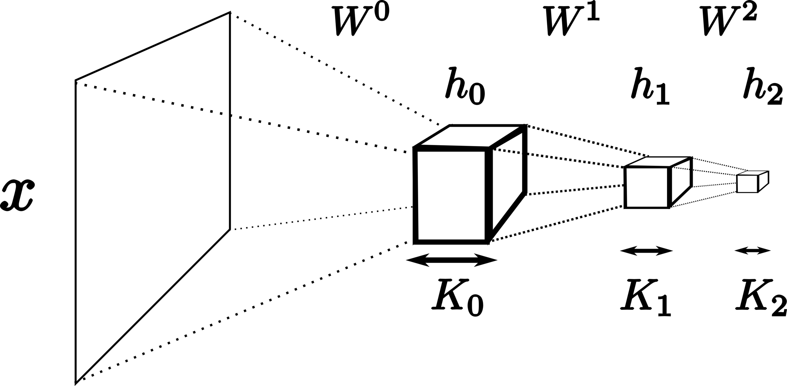
model - convolutions
model - convolutions
General pipeline
neural network
Dataset
loss function
gradient
update
Model
Method
data
label
- Introduction
- Data
- Model
- Method
- Conclusion
CONTENT
- Loss function
- Gradient Backpropagation (chain rule)
- Model update
method - loss function
method - loss function
Likelihood (Bernoulli distribution )
method - loss function
NN output
(pseudo proba)
pseudo-proba of being label
pseudo-proba of
being label
method - loss function
likelihood
labels
NN output
(pseudo proba)
method - loss function
likelihood
labels
NN output
(pseudo proba)
log-likelihood
method - loss function
likelihood
labels
NN output
(pseudo proba)
log-likelihood
negative
log-likelihood
- Introduction
- Data
- Model
- Method
- Conclusion
CONTENT
- Loss function
- Gradient Backpropagation (chain rule)
- Model update
Gradient of the loss with respect to the model parameters
method - gradient backpropagation
Gradient of the loss with respect to the model parameters
method - gradient backpropagation
Gradient of the loss with respect to the model parameters
method - gradient backpropagation
we want to increase
Gradient of the loss with respect to the model parameters
method - gradient backpropagation
we want to decrease
Gradient of the loss with respect to the model parameters
method - gradient backpropagation
we want to decrease
(a lot !)
How to compute the gradient of the loss with respect to each model parameter ?
chain rule
method - gradient backpropagation
Compute the gradient of the loss with respect to each model parameter using the chain rule (2-inputs example)
reminder
method - gradient backpropagation
gradient backpropagation
gradient vector contains
1 value for each parameter
method - gradient backpropagation
- Introduction
- Data
- Model
- Method
- Conclusion
CONTENT
- Loss function
- Gradient Backpropagation (chain rule)
- Model update
gradient descent
method - model update
gradient descent
method - model update
gradient descent
method - model update
gradient descent
method - model update
gradient descent
method - model update
method - model update
method - model update
- Introduction
- Data
- Model
- Method
- Conclusion
CONTENT
Conclusion
neural network
data
label
Dataset
loss function
gradient
update
Model
Method
neural network
data
label
data split
Model
Evaluation methodology
lock parameters
little break !