These are the slides for the introduction to geometric algebra as given on the ICRA2023 conference - in the workshop "Geometric Representations: The Roles of Modern Screw Theory, Lie algebra, and Geometric Algebra in Robotics".

They extensively use interactive animations made with the ganja.js library and its coffeeshop platform. (see https://enki.ws/ganja.js/examples/coffeeshop.html)

For full integration that synchronises animation timing with slide fragments, you have to copy paste the code below into your browser console. (copy the code, press shift+ctrl+j to open the console, hit paste and press enter).

// Broadcast slide fragment navigation to the iframe on the slide.
function broadcast(event) {
    var cur = Reveal.getIndices();
    var iFrame = [...document.querySelectorAll('iframe')].filter(x=>x.src)[0];
    if (iFrame) iFrame.contentWindow.postMessage([cur.h, cur.v, cur.f]+'',"*");
};

Reveal.addEventListener('fragmentshown', broadcast);
Reveal.addEventListener('fragmenthidden', broadcast);
Reveal.addEventListener('slidetransitionend', broadcast);

ICRA 2023

Geometric Algebra
Introduction for Robotics

Steven De Keninck

What is Geometric Algebra ?

An alternative to vector/matrix algebra ideal for (amongst many other things) geometry.

An algebra on a graded linear (vector) space, with an invertible product that operates on multivectors.

\(\oplus\)

\(\circlearrowleft\)

\(\oplus\)

\(\mathbb R\)

...

PSS

scalars

vectors

bivectors

pseudo scalar

ICRA 2023

What is Geometric Algebra ?

ICRA 2023

point

direction

line

plane

// construct lines
line_from_points (p1, p2)
line_from_points_and_dir (p, d)
line_from_plucker (a, b, c, d, e, f)

// construct planes
plane_from_points (p1, p2, p3)
plane_from_point_and_dirs (p, d1, d2)
plane_from_points_and_dir (p1, p2, d)
plane_from_point_and_line (p, l)
plane_from_equation (a, b, c, d)

// Intersections
intersect_line_plane (l, P)
intersect_plane_plane (P1, P2)
intersect_planes (P1, P2, P3)

// Projections
project_point_plane (p, P)
project_line_plane (l, P)
project_point_line (p, l)

position

rotation

matrix

quaternion

// construct transformations
mtx_translate (x, y, z)
mtx_rotate_euler (h, p, b)
mtx_rotate_axis_angle (x, y, z, a)
mtx_look_at (from, too, pole)

// apply transformations
transform_point (M, p)
transform_direction (M, d)
transform_line (M, l)
transform_plane (M, P)

// construct transformations
quat_from_euler (h, p, b)
quat_from_axis_angle (x, y, z, a)
quat_look_at (from, too, pole)
quat_from_matrix (M)
quat_to_matrix (Q)

// apply transformations
transform_point (Q, p)
transform_line (Q, l)
transform_plane (Q, P)

velocity

force

dual quaternion

// LA LA Land
factor_QR (M)
factor_LDL (M)
factor_SVD (M)
factor_LU (M)

// and even more code..
dquat_to_matrix (DQ)
dquat_from_matrix (M)
dquat_from_direction (d)
dquat_from_euler (h, p, b)

.. meshes ..
.. computational geometry .. 
.. keeps going ..

\( a \vee b \)

\( a \wedge b \)

\( (a \cdot b)b^{-1} \)

\(e^{ab}\)

\( ab\tilde a \)

\( \sqrt{ab^{-1}} \)

What is Geometric Algebra ?

We will first tackle the Algebra.

New numbers : Why do we need them?
New numbers : What are they ?
New numbers : How do I use them ?
\(k\)-vectors and Cayley Tables

ICRA 2023

الكتاب المختصر في حساب الجبر والمقابلة

al-Kitāb al-Mukhtaṣar fī Ḥisāb al-Jabr wal-Muqābalah

Muḥammad ibn Mūsā al-Khwārizmī

The Compendious Book on Calculation by Completion and Balancing

1. New Numbers: why do we need them?

ICRA 2023

Muḥammad ibn Mūsā al-Khwārizmī

1. New Numbers: why do we need them?

\(x^2 + 10x = 39\)

\(= 39\)

\(+ 25=64\)

\((x+5)^2 = 64\)

\(\Leftrightarrow x = 3\)

\(x\)

\(x^2\)

\(x\)

\(5\)

\(5x\)

\(x\)

\(5\)

\(5x\)

\(5\)

\(25\)

\( \begin{cases} \\ \\ \\ \\ \\ \\ \\ \\ \\ \\ \end{cases}\)

\(x+5\)

ICRA 2023

Muḥammad ibn Mūsā al-Khwārizmī

1. New Numbers: why do we need them?

\(ax^2 = bx\)

\(ax^2 = c\)

\(bx = c\)

\(ax^2 + bx = c\)

\(ax^2+c = bx\)

\(bx + c = ax^2\)

Why six equations ?????

No negative numbers, no zero !!

ICRA 2023

1. New Numbers: why do we need them?

Why six equations ?????

No negative numbers, no zero !!

\(x + 1 = 1\)

\(x + 1 = 0\)

zero!

negative numbers!

With 0 and negative numbers, we reduce the amount of equations from 6 to 1 !!!

ICRA 2023

\(\oplus\)

\(\circlearrowleft\)

\(\oplus\)

\(\mathbb R\)

...

PSS

scalars

vectors

bivectors

pseudo scalar

Transform point/line/plane/direction \(b\) with rotor \(a\)

\(ab\tilde a\)

Project any point/line/plane \(a\) on any point/line/plane \(b\)

\(\frac {a\cdot b} {b}\)

Compare this to the classic vector/matrix approach ...

// just a matrix multiply
transform_point( M,  )
// similar to point .. diff. M
transform_direction( M,  )
// should be 6x6 matrix
transform_line( M,  )
// similar to direction .. diff. M
transform_plane( M,  )

// none of these are similar..
project_point_line()
project_point_plane()
project_line_point()
project_line_plane()
project_plane_point()
project_plane_line()

Lets do the same with another simple equation..

x^2 \,\,+\,\, 1\,\, =\,\, 0

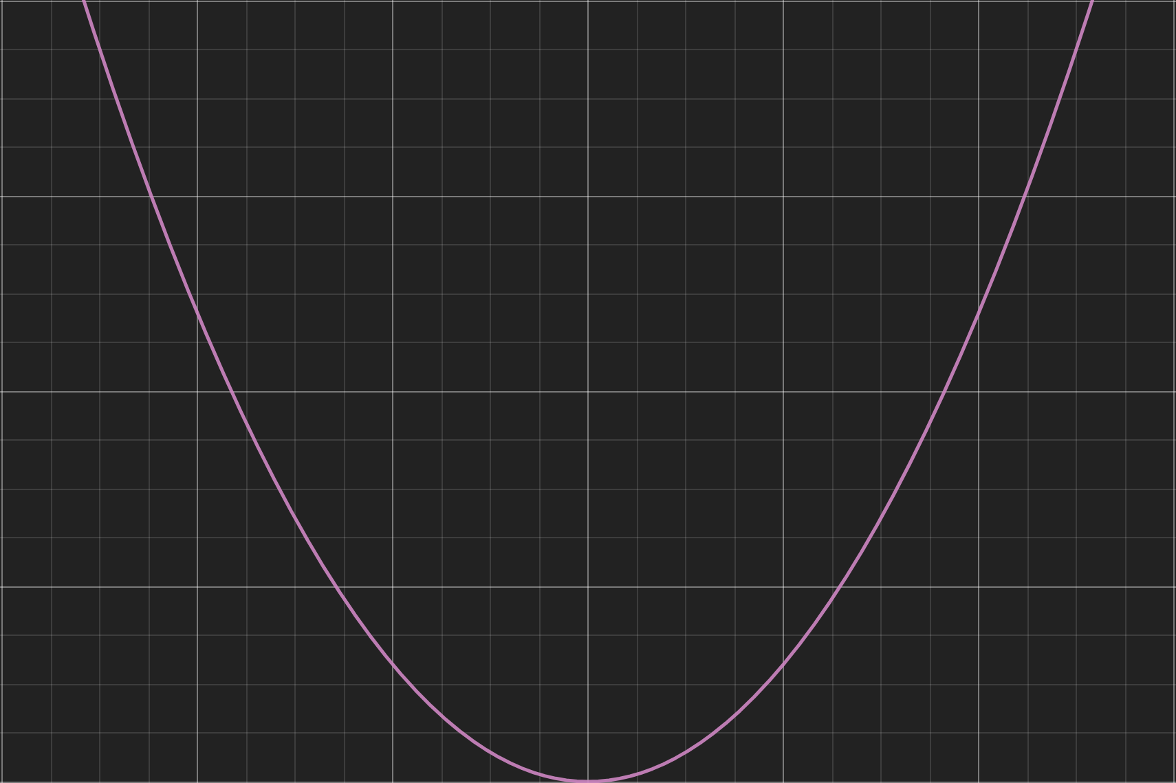
\(\mathbf e^2 = -1\)

\(\mathbf e^2 = +1\)

\(\mathbf e^2 = 0\)

\(\mathbb R_{\color{green}p\color{white},\color{red}q\color{white},\color{cyan}r\color{white}}\)

A Geometric Algebra is defined by this p,q,r signature specifying the metric of the n generators.

2. New Numbers: what are they?

ICRA 2023

\(\oplus\)

\(\circlearrowleft\)

\(\oplus\)

\(\mathbb R\)

...

PSS

scalars

vectors

bivectors

pseudo scalar

Transform point/line/plane/direction \(b\) with rotor \(a\)

\(ab\tilde a\)

Project any point/line/plane \(a\) on any point/line/plane \(b\)

\(\frac {a\cdot b} {b}\)

\(\mathbb R_{\color{green}p\color{white},\color{red}q\color{white},\color{cyan}r\color{white}}\)

A Geometric Algebra is defined by this p,q,r signature specifying the metric of the n generators.

\(\mathbb R_3 \)

\(\mathbf e_1, \mathbf e_2, \mathbf e_3 \), all square to \(+1\)

\(\mathbb R_{1,3} \)

\(\mathbf e_1\) squares to \(+1\), \(\mathbf e_2, \mathbf e_3, \mathbf e_4\), all square to \(-1\)

\(\mathbb R_{3,0,1} \)

\(\mathbf e_0\) squares to \(0\), \(\mathbf e_1, \mathbf e_2 ,\mathbf e_3\), all square to \(+1\)

We will use these generators to model vectors, points, circles, lines, planes, translations, boosts, rotations, screws, spheres, ...

\( \mathbf e_i \notin \mathbb R \qquad {\mathbf e_i}^2 \in \{0,1,-1\} \)

2. New Numbers: what are they?

ICRA 2023

3. New Numbers: how do I use them?

\( \mathbf e_i \notin \mathbb R \qquad {\mathbf e_i}^2 \in \{0,1,-1\} \)

\(x^2 \in \mathbb R\)

\((\alpha \mathbf e_1 + \beta \mathbf e_2)^2 \in \mathbb R\)

\(\alpha^2 \mathbf {e_1}^2 + \alpha\beta\color{lightgreen}\mathbf e_1\mathbf e_2\color{white} + \alpha\beta\color{lightgreen}\mathbf e_2\mathbf e_1 \color{white} + \beta^2 {\mathbf e_2}^2 \in \mathbb R\)

\( \color{lightgreen} \mathbf e_1\mathbf e_2 + \mathbf e_2\mathbf e_1 \color{white} = 0\)

\( \mathbf e_1\mathbf e_2 = - \mathbf e_2\mathbf e_1 \color{white} \)

\(\mathbf e_1\)

\(\mathbf e_2\)

\(x = \alpha \mathbf e_1 + \beta \mathbf e_2\)

ICRA 2023

\( \mathbf e_i \notin \mathbb R \qquad {\mathbf e_i}^2 \in \{0,1,-1\} \)

\( \mathbf e_1\mathbf e_2 = - \mathbf e_2\mathbf e_1 \)

3. New Numbers: how do I use them?

What is this new \(\mathbf e_1 \mathbf e_2 = \mathbf e_{12}\) element?

\(\alpha\mathbf e_1 + \beta\mathbf e_2\)

\(\alpha\mathbf e_{12}\)

\(\alpha\mathbf e_{123}\)

ICRA 2023

\( \mathbf e_i \notin \mathbb R \qquad {\mathbf e_i}^2 \in \{0,1,-1\} \)

\( \mathbf e_1\mathbf e_2 = - \mathbf e_2\mathbf e_1 \)

3. New Numbers: how do I use them?

\((\mathbf e_1 - \mathbf e_2)\mathbf e_1 = \)

\({\mathbf e_{12}}^2 = \)

\(\mathbf e_{123}\mathbf e_1 =\)

\(\frac 1 2 (\mathbf e_1 + \mathbf e_2) (\mathbf e_2 - \mathbf e_1) = \)

some exercises, with positive basis vectors.

\(\bf \frac 1 2 (e_{12} - 1 + 1 -e_{21} ) = e_{12}\)

\(\curvearrowleft\)

\(\bf e_{1231} = -e_{1213} = e_{1123} = e_{23}\)

\(\curvearrowleft\)

\(\bf e_1e_1 - e_2e_1 = 1 + e_{12}\)

\(\curvearrowleft\)

\(\bf e_{12} e_{12} = e_{1212} = - e_{1221} = -1\)

ICRA 2023

\( \mathbf e_i \notin \mathbb R \qquad {\mathbf e_i}^2 \in \{0,1,-1\} \)

\( \mathbf e_1\mathbf e_2 = - \mathbf e_2\mathbf e_1 \)

3. New Numbers: how do I use them?

The geometric product of two 3 dimensional vectors

\(v_1v_2 = (\color{lightblue}x_1\color{white}\color{lightgreen}x_2\color{white}+\color{lightblue}y_1\color{white}\color{lightgreen}y_2\color{white}+\color{lightblue}z_1\color{white}\color{lightgreen}z_2\color{white}) + (\color{lightblue}x_1\color{white}\color{lightgreen}y_2\color{white}-\color{lightblue}y_1\color{white}\color{lightgreen}x_2\color{white})\mathbf e_{12} + (-\color{lightblue}x_1\color{white}\color{lightgreen}z_2\color{white}+\color{lightblue}z_1\color{white}\color{lightgreen}x_2\color{white})\mathbf e_{31} + (\color{lightblue}y_1\color{white}\color{lightgreen}z_2\color{white}-\color{lightblue}z_1\color{white}\color{lightgreen}y_2\color{white})\mathbf e_{23}\)

\(\vec v_1 = \begin{bmatrix}\color{lightblue}x_1 \\ \color{lightblue} y_1 \\ \color{lightblue} z_1 \color{white}\, \end{bmatrix} \quad \vec v_2 = \begin{bmatrix}\color{lightgreen}x_2 \\ \color{lightgreen} y_2 \\ \color{lightgreen} z_2 \color{white}\, \end{bmatrix}\)

\( \underbrace{\qquad \qquad\qquad\qquad\qquad\qquad\qquad\qquad\qquad\qquad\qquad}\)

\( \cong \vec v_1 \times \vec v_2 \)

Cross Product !

\( \underbrace{\qquad \qquad\qquad\qquad}\)

\( \cong \vec v_1 \cdot \vec v_2 \)

Dot Product !

\(v_1 = (\color{lightblue}x_1\color{white}\mathbf e_{1} + \color{lightblue}y_1\color{white}\mathbf e_{2} + \color{lightblue}z_1\color{white}\mathbf e_{3} )\)

\(v_2 = ( \color{lightgreen}x_2\color{white}\mathbf e_{1} + \color{lightgreen}y_2\color{white}\mathbf e_{2} + \color{lightgreen}z_2\color{white}\mathbf e_{3})\)

ICRA 2023

\( \mathbf e_i \notin \mathbb R \qquad {\mathbf e_i}^2 \in \{0,1,-1\} \)

\( \mathbf e_1\mathbf e_2 = - \mathbf e_2\mathbf e_1 \)

3. New Numbers: how do I use them?

The geometric product of two 3 dimensional vectors

\( \underbrace{\qquad \qquad\qquad\qquad\qquad\qquad\qquad\qquad\qquad\qquad\qquad}\)

\( \cong \vec v_1 \times \vec v_2 \)

Cross Product !

\( \underbrace{\qquad \qquad\qquad\qquad}\)

\( \cong \vec v_1 \cdot \vec v_2 \)

Dot Product !

only scalar. 'Grade 0'.

\(v_1 \cdot v_2 = \langle v_1v_2 \rangle_0\)

only bivector. 'Grade 2'.

\(v_1 \wedge v_2 = \langle v_1v_2 \rangle_2\)

Note : One scalar and three imaginary parts. The geometric product of two vectors in \(\mathbb R_3\) is a quaternion!

ICRA 2023

\( \mathbf e_i \notin \mathbb R \qquad {\mathbf e_i}^2 \in \{0,1,-1\} \)

\( \mathbf e_1\mathbf e_2 = - \mathbf e_2\mathbf e_1 \)

3. New Numbers: how do I use them?

The geometric product of two 3 dimensional vectors

only scalar. 'Grade 0'.

\(v_1 \cdot v_2 = \langle v_1v_2 \rangle_0\)

only bivector. 'Grade 2'.

\(v_1 \wedge v_2 = \langle v_1v_2 \rangle_2\)

\(v_1v_2 = v_1 \cdot v_2 + v_1 \wedge v_2 \)

*famous, but be careful! only if \(v_1\) or \(v_2\) is vector!

ICRA 2023

\( \mathbf e_i \notin \mathbb R \qquad {\mathbf e_i}^2 \in \{0,1,-1\} \)

\( \mathbf e_1\mathbf e_2 = - \mathbf e_2\mathbf e_1 \)

3. New Numbers: how do I use them?

\(v_1v_2 = v_1 \cdot v_2 + v_1 \wedge v_2 \)

In general, the geometric product between a grade \(s\) multivector \(\bf a\) and a grade \(t\) multivector \(\bf b\) has grades from \(|s-t|\) to \(s+t\) in steps of 2.

The highest and lowest grade parts are often useful and are called the wedge and dot products respectively.

\( \langle a \rangle_s \cdot \langle b \rangle_t = \langle ab \rangle_{|s-t|}\)

\( \langle a \rangle_s \wedge \langle b \rangle_t = \langle ab \rangle_{s+t}\)

ICRA 2023

\( \mathbf e_i \notin \mathbb R \qquad {\mathbf e_i}^2 \in \{0,1,-1\} \)

\( \mathbf e_1\mathbf e_2 = - \mathbf e_2\mathbf e_1 \)

3. New Numbers: how do I use them?

There are even more products from other branches of mathematics and physics

that map to some combination of or grade selection of the geometric product!

\( \langle a \rangle_s \cdot \langle b \rangle_t = \langle ab \rangle_{|s-t|}\)

\( \langle a \rangle_s \wedge \langle b \rangle_t = \langle ab \rangle_{s+t}\)

\(( a \vee b)^* = a^* \wedge b^*\)

\( a \times b = \frac 1 2 (ab - ba)\)

The Geometric Product

The Wedge Product

The Dot Product

The Vee Product

The Commutator Product

ICRA 2023

\(\oplus\)

\(\circlearrowleft\)

\(\oplus\)

\(\mathbb R\)

...

PSS

scalars

vectors

bivectors

pseudo scalar

4. Cayley Tables !

\( \mathbf e_i \notin \mathbb R \qquad {\mathbf e_i}^2 \in \{0,1,-1\} \)

\( \mathbf e_1\mathbf e_2 = - \mathbf e_2\mathbf e_1 \)

ICRA 2023

First, let us review the geometry of arrows, and the vector algebra operators.

but does this still work if we use arrows to represent points?

For the geometry of arrows, these operations are all well defined. Given just the orange inputs, you can reconstruct the green output.

Two points define a line. AND NOTHING ELSE!

⇒ EVERY binary operation between two points is a one dimensional operation!

ICRA 2023

The First Postulate

Two points define a line. AND NOTHING ELSE!

⇒ EVERY binary operation between two points is a one dimensional operation!

so, for points \(A,B\), all operations \(A+B, A-B, AB, A \wedge B, A \vee B, ...\) must produce a result on the line between \(A\) and \(B\) (or zero). In general, the types of elements determine exactly the set of geometrically plausible outputs.

Can we set things up so that all operators always produce geometrically valid outcomes?

ICRA 2023

The First Postulate

Can we set things up so that all operators always produce geometrically valid outcomes?

A+A ?

AA ?

The result must be a point again, and it can only be at that position!

⟶ every 'algebra of geometry' MUST be homogeneous!

⟶ A+A = 2A still A, but twice as happy.

If you only have one point, then any transformation is the identity!

⟶ AA \(\cong\) 1 , the transformation that takes A to A.

⟶ if AA is identity, then A is an involutory transformation. A is a reflection!

ICRA 2023

The First Postulate

Can we set things up so that all operators always produce geometrically valid outcomes?

A+B ?

The result must be a point, for equally happy A,B it will be halfway.

A+B

AB ?

With A and B point reflections (and points), AB is a translation (try it!)

ABA ?

The point B reflected in A.

BAB ?

The point A reflected in B.

ABA

BAB

ICRA 2023

The First Postulate

Can we set things up so that all operators always produce geometrically valid outcomes?

A+B ?

A+B

AB ?

ABA ?

BAB ?

\(x=1 \iff x-1=0\)

\(\mathbf e_1 - \mathbf e_0\)

\(\mathbf e_1 - 2\mathbf e_0\)

\((\mathbf e_1 - \mathbf e_0) + (\mathbf e_1 - 2\mathbf e_0) = \mathbf 2e_1 - \mathbf 3e_0 \) \(\iff 2x - 3 = 0 \iff x = 1.5\)

\((\mathbf e_1 - \mathbf e_0) (\mathbf e_1 - 2\mathbf e_0) = 1 - 2\mathbf e_{10} - \mathbf e_{01} = 1 + \mathbf e_{01} \)

\((\mathbf e_1 - \mathbf e_0) (\mathbf e_1 - 2\mathbf e_0) (\mathbf e_1 - \mathbf e_0)= \mathbf e_1\) \(\iff x = 0\)

\((\mathbf e_1 - \mathbf e_0) (\mathbf e_1 - 2\mathbf e_0) (\mathbf e_1 - \mathbf e_0)= \mathbf e_1 - 3\mathbf e_0\) \(\iff x = 3\)

ABA

BAB

\(x=2 \iff x-2=0\)

ICRA 2023

The First Postulate

Can we set things up so that all operators always produce geometrically valid outcomes?

What if we move to a new viewpoint?

It is possible our points weren't points at all! This however can not change the behavior we saw from our original point of view!

The equivalence principle : if you can make it look like a duck, it'll quack.

ICRA 2023

The First Postulate

Can we set things up so that all operators always produce geometrically valid outcomes?

The equivalence principle : if you can make it look like a duck, it'll quack.

If points are point reflections, lines must be line reflections!
The product of parallel lines must be a translation!
Our reflection formula works for points and lines!

ICRA 2023

The First Postulate

Can we set things up so that all operators always produce geometrically valid outcomes?

Now that we know lines must be line reflections we can check bi-reflections easily ..

Rotation

Translation

Point Reflection

Bireflections have a gauge degree of freedom.

ICRA 2023

The First Postulate

Can we set things up so that all operators always produce geometrically valid outcomes?

\(\mathbf e_1 + \mathbf e_0\)

\(\mathbf e_{12} + \mathbf e_{02}\)

\(\rightarrow x = -1\)

same vector, different geometry!

still the same point reflection!

\(\mathbf e_{12} + \mathbf e_{02} = (\mathbf e_1 + \mathbf e_0)\mathbf e_2\)

\( x = -1\)

\( y = 0\)

\(\rightarrow\) Product of two orthogonal vectors is a pure bivector. Reflecting in two orthogonal mirrors is a point reflection in their intersection point.

ICRA 2023

The First Postulate

Can we set things up so that all operators always produce geometrically valid outcomes?

A+B

A-B

The sum of two elements is their bisector, the element halfway in between.

The difference of two elements is the other bisector, for parallel elements, it is at infinity!

ICRA 2023

The First Postulate

At this point, we have an actual algebra of geometry. Our set of elements are the point(reflection)s, line(reflection)s, plane(reflection)s, ... multiplication with scalars, addition and multiplication between elements all are always geometrically valid!

But, we are not done yet - to get an intuitive understanding we still need a way to visualize all the different products - and for that the Geometric Gauges are key!

ICRA 2023

Can we set things up so that all operators always produce geometrically valid outcomes?

Reflections are the fundamental building blocks for Euclidean geometry in any #D

The First Postulate

ICRA 2023

The First Postulate

After picking the viewpoint where things look most simple, we will use the gauges to understand exactly what all of the products do geometrically.

reflection/line

reflection/point

rotation

translation

when combining reflections, only the relative position matters.

e.g. any set of orthogonal line-reflections through a point produces the same point-reflection.

this gives us a 'geometric gauge' degree of freedom, which we can use to understand all the different products.

ICRA 2023

The First Postulate

After picking the viewpoint where things look most simple, we will use the gauges to understand exactly what all of the products do geometrically.

The geometric product eliminates identical mirrors.

ICRA 2023

The First Postulate

After picking the viewpoint where things look most simple, we will use the gauges to understand exactly what all of the products do geometrically.

The geometric product eliminates identical mirrors.

The dot product eliminates parallel mirrors.

ICRA 2023

The First Postulate

After picking the viewpoint where things look most simple, we will use the gauges to understand exactly what all of the products do geometrically.

The geometric product eliminates identical mirrors.

The dot product eliminates parallel mirrors.

The regressive product keeps identical mirrors.

ICRA 2023

The First Postulate

After picking the viewpoint where things look most simple, we will use the gauges to understand exactly what all of the products do geometrically.

The geometric product eliminates identical mirrors.

The dot product eliminates parallel mirrors.

The regressive product keeps identical mirrors.

The outer product finds orthogonal mirrors.

ICRA 2023

The First Postulate

After picking the viewpoint where things look most simple, we will use the gauges to understand exactly what all of the products do geometrically.

The geometric product eliminates identical mirrors.

The dot product eliminates parallel mirrors.

The regressive product keeps identical mirrors.

The outer product finds orthogonal mirrors.

ICRA 2023

The First Postulate

After picking the viewpoint where things look most simple, we will use the gauges to understand exactly what all of the products do geometrically.

The geometric product eliminates identical mirrors.

The dot product eliminates parallel mirrors.

The regressive product keeps identical mirrors.

The outer product finds orthogonal mirrors.

Cartan-Dieudonne :

Every orthogonal transformation in an n-dimensional symmetric bilinear space can be described as the composition of at most n reflections.

ICRA 2023

The First Postulate

\(ab\) Geometric Product composes reflections

\(a\wedge b\) Outer Product Intersects elements

\(a\vee b\) Regressive Product joins elements

\(a\cdot b\) Dot Product rejects elements

ICRA 2023

The First Postulate

Now, lets see it in action!

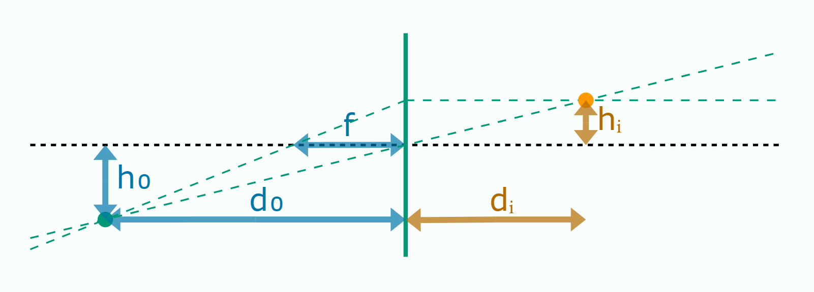
\(d_i = \big ( \frac 1 f - \frac 1 {d_0} \big )^{-1}\qquad h_i=-\frac {d_i} {d_0} h_0\)

ICRA 2023

The First Postulate

\(d_i = \big ( \frac 1 f - \frac 1 {d_0} \big )^{-1}\qquad h_i=-\frac {d_i} {d_0} h_0\)

The paraxial approximation of the thin lens equation

ICRA 2023

The First Postulate

\(d_i = \big ( \frac 1 f - \frac 1 {d_0} \big )^{-1}\qquad h_i=-\frac {d_i} {d_0} h_0\)

The paraxial approximation of the thin lens equation

\(\vec a = \overline {\vec c - \vec f}\)

\(\vec b= \vec c - \vec p\)

\(d_0 = \vec a \cdot \vec b\)

ICRA 2023

The First Postulate

\(d_i = \big ( \frac 1 f - \frac 1 {d_0} \big )^{-1}\qquad h_i=-\frac {d_i} {d_0} h_0\)

The paraxial approximation of the thin lens equation

\((\overline {\vec c - \vec f}) \, \cdot\)

\((\vec c - \vec p)\)

\(d_0 = \)

\(h_0 = (\overline{\vec c - \vec g} )\,\cdot\,(\vec c - \vec p) \)

ICRA 2023

The First Postulate

The paraxial approximation of the thin lens equation

There are no coefficients or even ratios, and the formula can be read from left to right.

ICRA 2023

The First Postulate

The paraxial approximation of the thin lens equation

\( p \vee f \) = line through p and f
\((p \vee f) \wedge L\) = intersection with lens
\((p \vee f) \wedge L \cdot L \) = line orthogonal to L
\((p \vee f) \wedge L \cdot L \wedge (p \vee c)\) = intersect with line through center

\(\vee\) = join \(\wedge\) = meet \(\bullet\) = dot

ICRA 2023

The First Postulate

The paraxial approximation of the thin lens equation

ICRA 2023

The First Postulate

Thanks!

There are still many things left uncovered, but they all build on the same simple ideas.