Random fields on the sphere using SFEM
Erik Jansson

Joint work with Annika Lang and Mihály Kovács
Some motivation...
- \(\left(\kappa^2-\Delta_{\mathbb{S}^2}\right)^\beta u=\mathcal{W}\)
- Is it possible to approximate \(u\) using low-order conforming finite elements?
Some motivation...
- \(\left(\kappa^2-\Delta_{\mathbb{S}^2}\right)^\beta u=\mathcal{W}\)
- Is it possible to approximate \(u\) using low-order conforming finite elements?
- In other words, a FEM based simulation method!
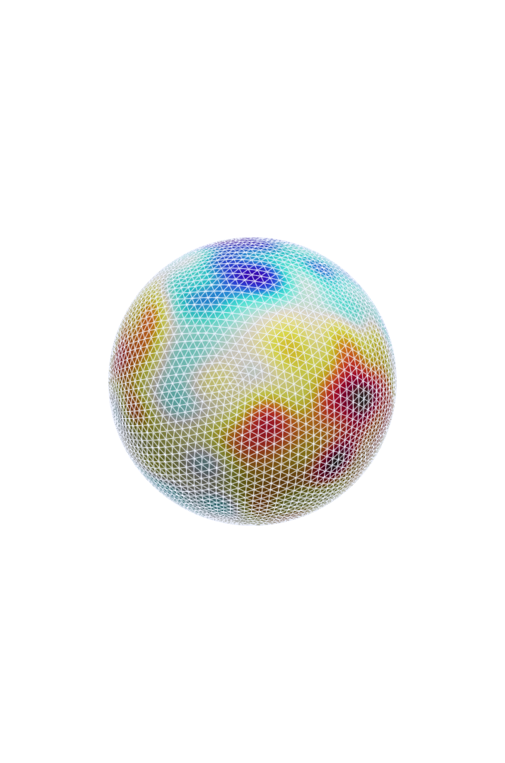
- Surface: The 2-sphere, \(\{|x|=1, x \in \mathbb{R}^3\}\)
- Operator: \(\mathcal{L}=(\kappa^2-\Delta_{\mathbb{S}^2})\)
- Problem for RF simulation: \(\mathcal{L}^\beta u =\mathcal{W}\), \( \beta >0.5\)
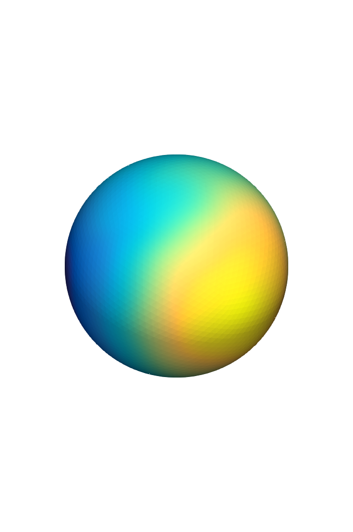
- For now, let RHS \(F \in L^2(\mathbb{S}^2)\) be deterministic!
Setting
\mathcal{L}^\beta u=F,~~F \in L^2(\mathbb{S}^2)
\mathcal{L}^\beta u=F
\mathcal{L} u^1=F
\mathcal{L}^{\beta-1} u=u^1
\mathcal{L} u^1=F
\mathcal{L} u^2=u^1
\mathcal{L}^{\beta-2} u=u^2
\mathcal{L} u^1=F
\mathcal{L} u^2=u^1
\mathcal{L} u^3=u^2
\vdots
\mathcal{L}^{\{\beta\}} u=u^{\left \lfloor{\beta}\right \rfloor }
Split problems to obtain recursion!
Two types of problems!
Several linear elliptic problems...
...and one fractional elliptic problem
Fractional problem
What to do with \(\mathcal{L}^{\{\beta\}}\)?
\mathcal{L}^{-\{\beta\}} =\frac{\sin( \pi \{\beta\})}{\pi}\int_{-\infty}^{\infty} e^{2 \{\beta\} y} \left( I+e^{2y}\mathcal{L}\right)^{-1} \, \mathrm{d} y\\
\mathcal{L}^{-\{\beta\}} \approx Q^{\{\beta\}}_k= \frac{2 k \sin(\pi \{\beta\})}{\pi} \sum_{l=-K^{-}}^{K^+} e^{2\{\beta\} y_{l}} \color{white}{\left(I+e^{2 y_l}\mathcal{L}\right)^{-1}} \\
\color{white}{u \approx u_{Q,k}= Q^{\{\beta\}}_k u^{\lfloor\beta \rfloor}}
\mathcal{L}^{-\{\beta\}} =\frac{\sin( \pi \{\beta\})}{\pi}\int_{-\infty}^{\infty} e^{2 \{\beta\} y} \left( I+e^{2y}\mathcal{L}\right)^{-1} \, \mathrm{d} y\\
\mathcal{L}^{-\{\beta\}} \approx Q^{\{\beta\}}_k= \frac{2 k \sin(\pi \{\beta\})}{\pi} \sum_{l=-K^{-}}^{K^+} e^{2\{\beta\} y_{l}} \color{forestgreen}{\left(I+e^{2 y_l}\mathcal{L}\right)^{-1}} \\
\color{white}{u \approx u_{Q,k}= Q^{\{\beta\}}_k \color{ForestGreen}u^{\lfloor\beta \rfloor}}
\(\|u-u_{Q,k}\|\) decays exponentially in \(k\)
\mathcal{L}^{-\{\beta\}} =\frac{\sin( \pi \{\beta\})}{\pi}\int_{-\infty}^{\infty} e^{2 \{\beta\} y} \left( I+e^{2y}\mathcal{L}\right)^{-1} \, \mathrm{d} y\\
\mathcal{L}^{-\{\beta\}} \approx Q^{\{\beta\}}_k= \frac{2 k \sin(\pi \{\beta\})}{\pi} \sum_{l=-\color{ForestGreen}{K^{-}}}^{\color{ForestGreen}{K^+}} e^{2\{\beta\} y_{l}} \color{forestgreen}{\left(I+e^{2 y_l}\mathcal{L}\right)^{-1}} \\
\color{white}{u \approx u_{Q,k}= Q^{\{\beta\}}_k \color{ForestGreen}u^{\lfloor\beta \rfloor}}
Finite elements for linear problems on surfaces
What to do with \(\mathcal{L}\)?
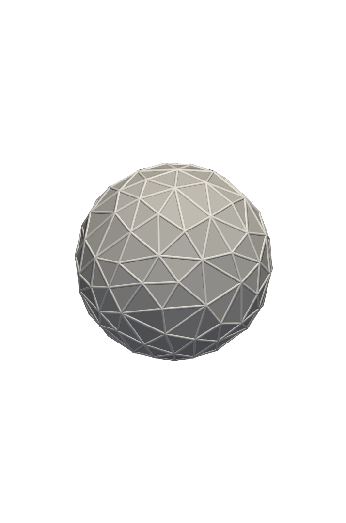
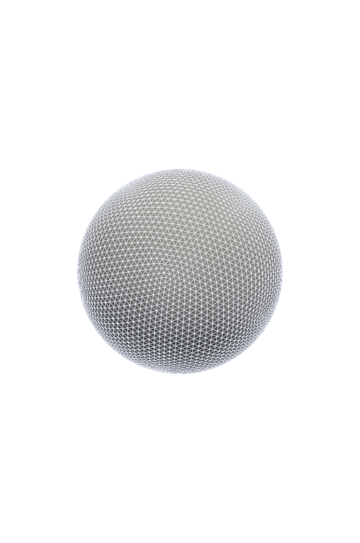
Step 1:
Approximate \(\mathbb{S}^2\) with triangles, \(\mathbb{S}^2_h\)
Step 2:
Decide on FEM space \(S_h\)
Step 2:
Decide on FEM space \(S_h\)
Continuous
Step 2:
Decide on FEM space \(S_h\)
Continuous
Piecewise affine
Step 3:
How to compare functions on \(\mathbb{S}^2\) and \(\mathbb{S}^2_h\)?
Lift them!
Lift them!
p(x)=x-(\|x\|_{\mathbb{R}^3}-1)\nu(x)
Given \(\eta: \mathbb{S}^2_h \to \mathbb{R}\), \(\eta^\ell= \eta \circ p^{-1}\) is on \(\mathbb{S}^2\)!
Recall the recursion from earlier
\mathcal{L} u^1=F
\mathcal{L} u^2=u^1
\mathcal{L} u^3=u^2
\vdots
\mathcal{L}^{\{\beta\}} u=u^{\left \lfloor{\beta}\right \rfloor }
\mathfrak{a}_{\mathbb{S}^2_h}(u_h^1,v)=(F_h,v)_{L^2(\mathbb{S}^2_h)}
\mathfrak{a}_{\mathbb{S}^2_h}(u_h^2,v)=(u^1_h,v)_{L^2(\mathbb{S}^2_h)}
\mathfrak{a}_{\mathbb{S}^2_h}(u_h^3,v)=(u^2_h,v)_{L^2(\mathbb{S}^2_h)}
\mathfrak{a}_{\mathbb{S}^2_h,l}(u_{h,l},v)=(u^{\lfloor\beta\rfloor}_{h},v )_{L^2(\mathbb{S}^2_h)}
\vdots
\mathfrak{a}_{\mathbb{S}^2_h,l}(u_{h,l},v)=(u^{\lfloor\beta\rfloor}_{h},v )_{L^2(\mathbb{S}^2_h)}
Solve final problem \(K^++K^-+1\) times and sum up to obtain \(u_{h}\)!
\mathfrak{a}_{\mathbb{S}^2_h}(u_h^1,v)=(F_h,v)_{L^2(\mathbb{S}^2_h)}
\mathfrak{a}_{\mathbb{S}^2_h}(u_h^2,v)=(u^1_h,v)_{L^2(\mathbb{S}^2_h)}
\mathfrak{a}_{\mathbb{S}^2_h}(u_h^3,v)=(u^2_h,v)_{L^2(\mathbb{S}^2_h)}
\vdots
SFEM Error
\|u-u_{h}^\ell\| \leq C \left( h^2 \|F\|{+}\|F-F_h^\ell\|\right)
SFEM Error
\|u-u_{h}^\ell\| \leq C \left( h^2 \|F\|{+}{\color{ForestGreen}{\|F-F_h^\ell\|}}\right)
The discretization of the geometry introduces an additional term!
SFEM Recursion Error
\|u_{l}{-}u_{h,l}^\ell\|
{\leq} C \left(h^2 \|u^{\lfloor \beta \rfloor }\|
{+}\|u^{\lfloor \beta \rfloor }{-}u_{h}^{\lfloor \beta \rfloor ,\ell}\|\right)
SFEM Recursion Error
SFEM Recursion Error
\|u_{l}{-}u_{h,l}^\ell\|
{\leq} C \left(h^2 \|u^{\lfloor \beta \rfloor }\|
{+}{\color{ForestGreen}{\|u^{\lfloor \beta \rfloor }{-}u_{h}^{\lfloor \beta \rfloor ,\ell}\|}}\right)
\color{ForestGreen}{\|u^{\lfloor \beta \rfloor }{-}u_{h}^{\lfloor \beta \rfloor ,\ell}\|} \color{white}{{\leq} C\left(h^2 \|u_L^{\lfloor \beta \rfloor -1}\|{+}\|u_L^{\lfloor \beta \rfloor -1}{-}u_{L,h}^{\lfloor \beta \rfloor-1 ,\ell}\|\right)}
The error from the geometry discretization is the error of the previous problem in the recursion!
SFEM Recursion Error
\|u_{l}{-}u_{h,l}^\ell\|
{\leq} C \left(h^2 \|u^{\lfloor \beta \rfloor }\|
{+}{\color{ForestGreen}{\|u^{\lfloor \beta \rfloor }{-}u_{h}^{\lfloor \beta \rfloor ,\ell}\|}}\right)
Random fields simulation algorithm
1. Let \(F=\mathcal{W}\)
2. Solve \(\mathcal{L}^\beta u = \mathcal{W}\)
1. Let \(F=\mathcal{W}\)
3. Solve \(\mathcal{L}^\beta u_L = \mathcal{W}_L\)
2. Approximate \(\mathcal{W}\) with \(\mathcal{W}_L\)
\mathcal{W}\sim \sum_{l=1}^\infty\sum_{m=-l}^l a_{l,m}Y_{l,m}
\mathcal{W}_L= \sum_{l=1}^L\sum_{m=-l}^l a_{l,m}Y_{l,m}
2. Approximate \(\mathcal{W}\) with \(\mathcal{W}_L\)
\mathcal{W}_L= \sum_{l=1}^L\sum_{m=-l}^l a_{l,m}Y_{l,m}
\|u-u_L\|_* \leq C_{\kappa}\left(\frac{1}{2\beta-1}+\frac{1}{4\beta-1}\right)L^{1-2\beta}
2. Approximate \(\mathcal{W}\) with \(\mathcal{W}_L\)
~\\
\|u-u_{L,h}^{\ell}\|_* \leq C(L+1)\left({L^{-2\beta}}{+e^{-\pi^2/(4k)}+ h^s(L+1)^{s}}\right)\\
~
Error For Noise Simulation
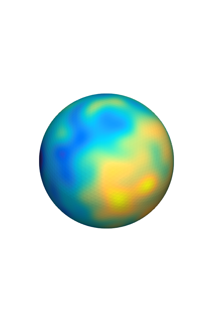
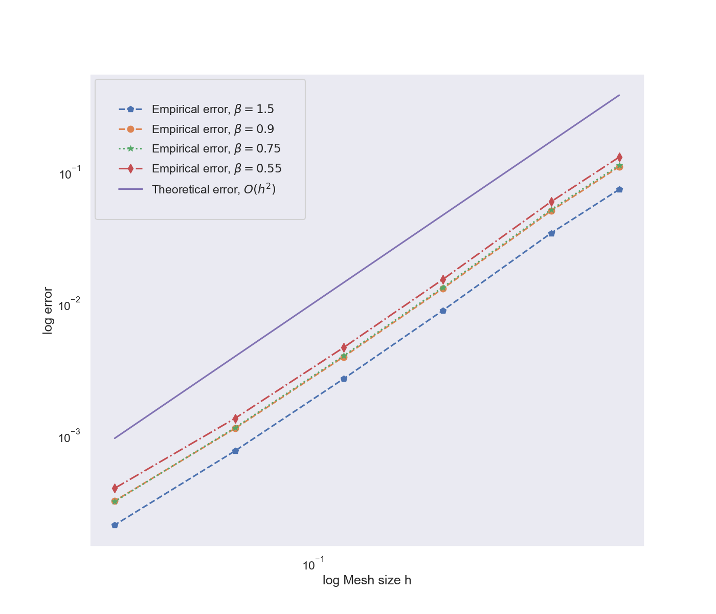
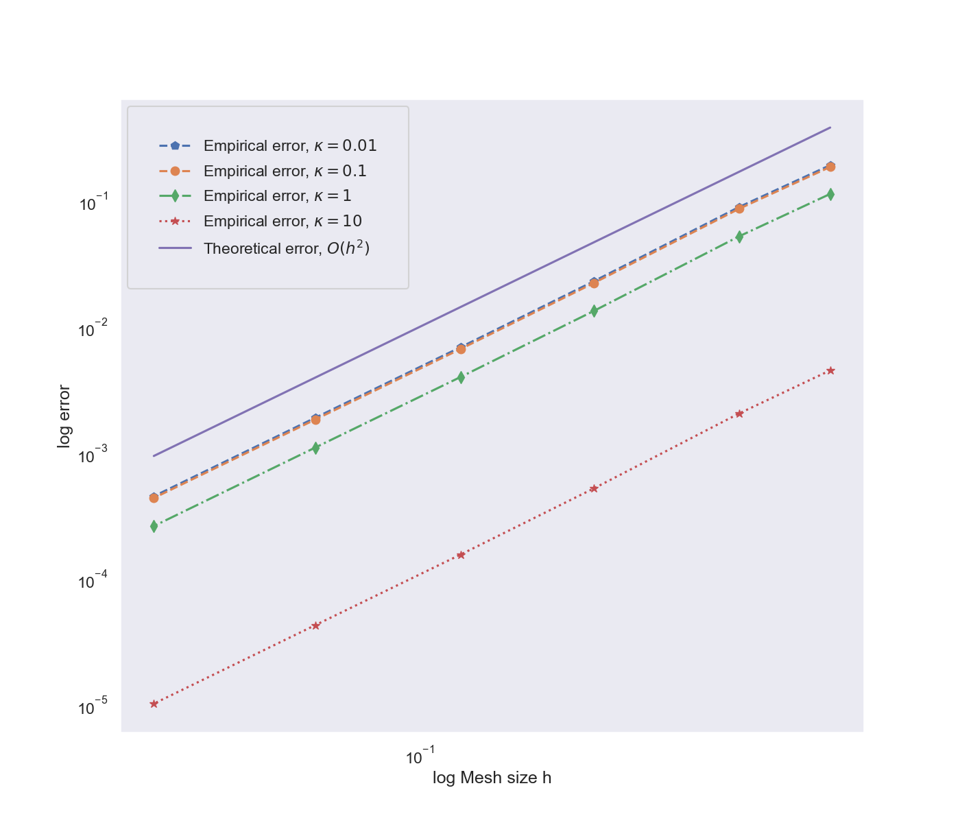
Numerical results
- \((\kappa^2-\Delta_{\mathbb{S}^2})^\beta u_1=\mathcal{W}_1\)
- Monte-Carlo estimate of \(L^2(\Omega;L^2(\mathbb{S}^2))\)-norm
- With good parameters: Expect to see error decrease as \(h^2\)
- Use for instance FEniCS!
Numerical results
- \((\kappa^2-\Delta_{\mathbb{S}^2})^\beta u_1=\mathcal{W}_1\)
- Monte-Carlo estimate of \(L^2(\Omega;L^2(\mathbb{S}^2))\)-norm
- With good parameters: Expect to see error decrease as \(h^2\)
- Use for instance FEniCS!
Thank you!