An exponential-free structure preserving integrator for stochastic Lie–Poisson systems
Erik Jansson
DAMTP, University of Cambridge and Wolfson College

Joint work with:
- Annika Lang (Chalmers/University of Gothenburg)
- Sagy Ephrati Imperial College London
- Erwin Luesink (University of Amsterdam )
Made possible by:
-
Klas Modin and Milo Viviani. Lie–Poisson methods for isospectral flows. Foundations of Computational Mathematics, 20:889–921, 2020.
- Grigori N. Milstein and Michael V. Tretyakov. Stochastic Numerics for Mathematical Physics. Springer Berlin Heidelberg, 2004.
- Charles-Edouard Bréhier, David Cohen, and Tobias Jahnke. Splitting integrators for stochastic Lie–
Poisson systems. Mathematics of Computation, 92(343):2167–2216, 2023.
Talk based on:
asdasdasd


arxiv:2408.16701

Examples of systems
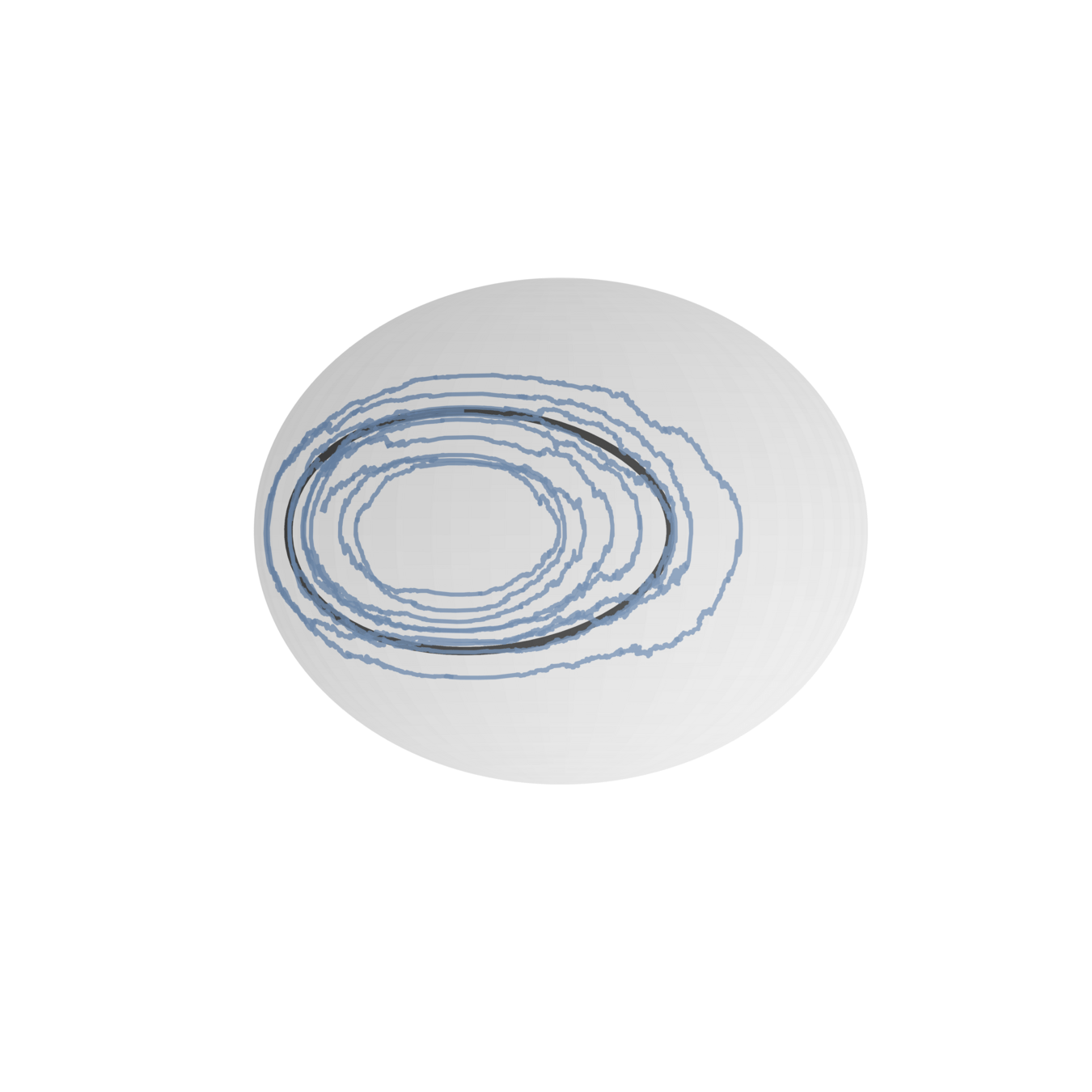
Stochastic rigid body
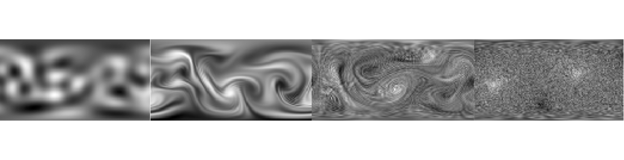
Stochastic (sine) Euler equations
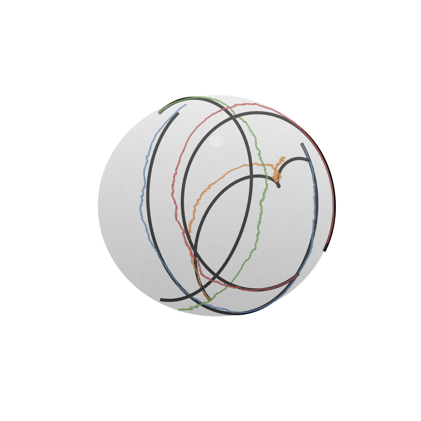
Stochastic point vortex dynamics
Lie-Poisson systems
Lie group \(G\) with algebra \(\mathfrak{g}\)
Hamiltonian \(H\colon \mathfrak{g}^* \to \mathbb R\)
Two ingredients
Important geometric structure:
LP Systems evolve on coadjoint orbits
(symplectic manifolds that foliate space!)
+ Several preserved quantities, Hamiltonian, Casimirs etc.
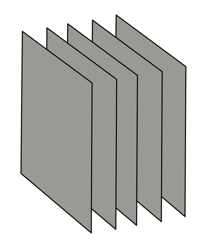
Coadjoint orbits
Dynamics on orbit
Lie-Poisson systems
\(G \subset \operatorname{GL}(n)\) is compact, simply connected and \(J\)-quadratic, i.e., \(A \in \mathfrak{g} \iff AJ + JA^* = 0 \)
Examples: \(\mathfrak{so}(N), \mathfrak{su}(N), \mathfrak{sp}(N)\).
In this setting, LP flow is isospectral:
Lie-Poisson systems
Example of LP systems
Classic example: rigid body (ODE)
- Algebra: \(\mathfrak{so}(3) \cong \mathbb R^3\)
- Bracket: \([v,w] = w \times v\)
- Hamiltonian: \(H(v) = v \cdot Iv\)
Introducing stochasticisty
How to add noise to equations?
- \(M\) independent scalar Brownian motions \(W^1, \ldots, W^M\)
- \(M\) noise Hamiltonians \(H_k\colon\mathfrak{g}^*\to \R\)
Why Strato?
Why these coefficients?
We need a chain rule
Same bracket-type coefficient: same geometric structure
Stochastic LP Systems evolve on coadjoint orbits and have Casimirs!
Introducing stochasticisty
Stochastic LP Systems evolve on coadjoint orbits and have Casimirs!
Coadjoint orbits
With transport noise
With non-transport noise
Introducing stochasticisty
Geometric structure is needed
What to assume to prove the existence of solutions?
E.g. Lipschitz is not realistic to assume
But! Some smoothness is sufficient for global existence
System remains on compact level sets of Casimirs
\(\rightarrow\) truncation argument to prove existence
Structure preservation: accurate numerics
Classic example: rigid body
- Algebra: \(\mathfrak{so}(3) \cong \mathbb R^3\)
- Bracket: \([v,w] = w \times v\)
Off the shelf integrator?
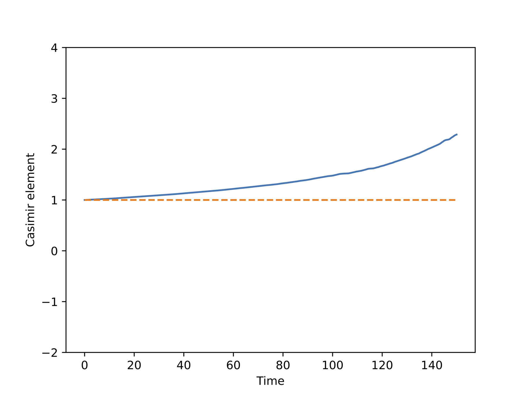
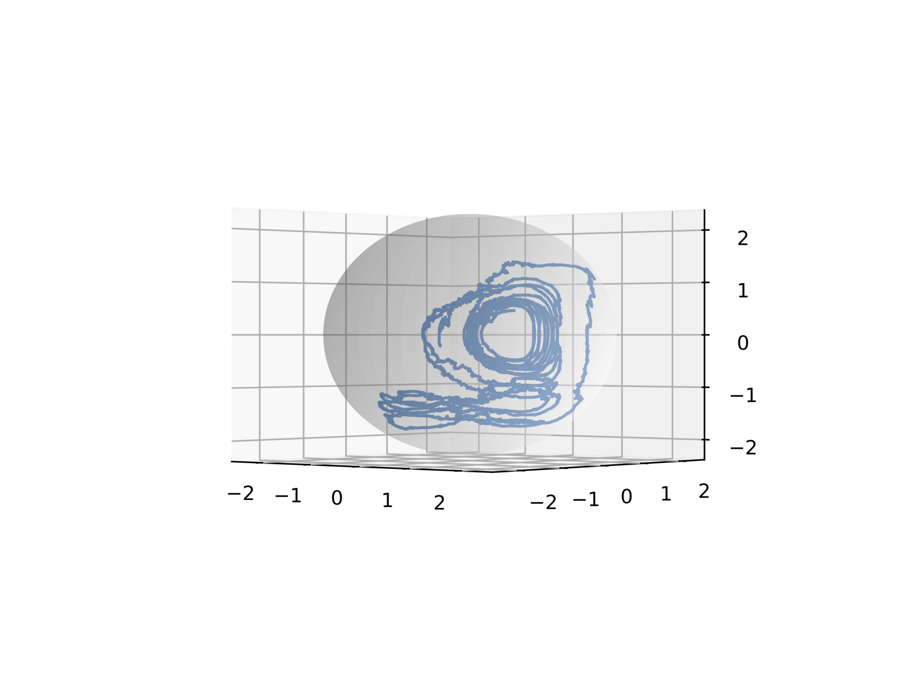
Non-physical behavior!
Structure preservation: accurate numerics
Structure-preserving integrators?
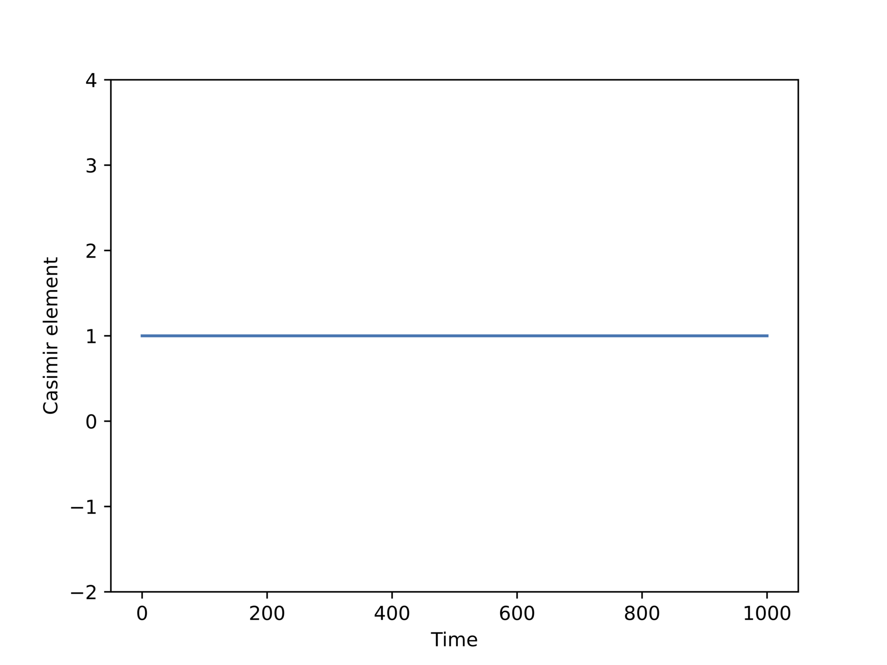
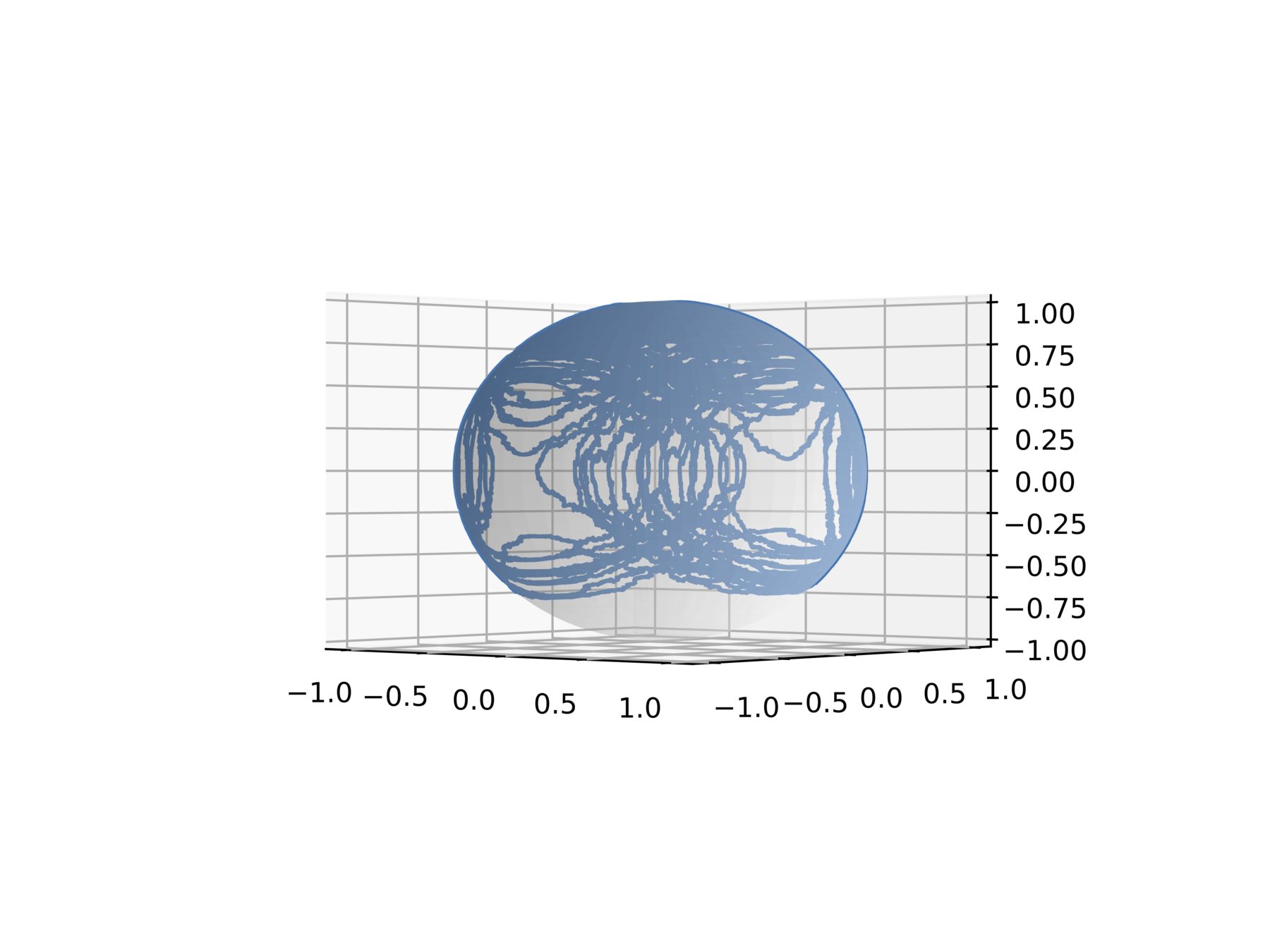
Structure preservation: accurate numerics
Wish list:
- Preserve Casimirs a.s.
- Preserve symplectic structure on coadjoint orbits a.s.
= Lie–Poisson integrator
Also: Avoid exponential map! (expensive, matrices in our applications are \(\sim2000\times2000\) )
Structure preservation: accurate numerics
Unreducing LP systems
LP systems on \(\mathfrak{g}^*\) are reductions of Hamiltonian systems on \(T^*G \cong G \times \mathfrak{g}^*\)
\(H\colon \mathfrak{g}^* \to \mathbb R\) lifts to left-invariant Hamiltonian!
\(G\) acts on \(T^*G\) by \(g.(Q,P) = (gQ,g^{-*}P)\)
Associated momentum map:
Do for all Hamiltonians!
Note: No a priori guarantee that this system remains on \(T^*G\)!
Embedded into \((R^{n \times n})^2\)
However! Remains on \(T^*G\)
Unreducing LP systems
\(X_t = \mu(Q_t,P_t) \in \mathfrak{g}^*\) satisfies
Unreducing LP systems
\(\Phi_h \colon T^*G \to T^* G\): \(G\)-equivariant symplectic integrator \(\rightarrow\)
Reduces to a Lie–Poisson integrator by \(\mu\)
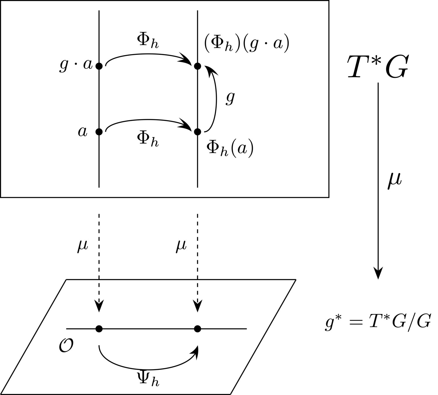
Exploit the unreduction!
Deriving the integrator
Do we know such an integrator?
Implicit midpoint!
- Symplectic
- Equivariant
- Well studied

Deriving the integrator
Stochastic isospectral midpoint:
Take \(Q_n,P_n\) such that \(\mu(Q_n,P_n) = X_n\)
Take \(X_{n+1} = \mu(\Phi_h(Q_n,P_n))\)
Deriving the integrator
Error analysis: essentially without crying
Exploit the unreduction!
Check the literature for error analysis for implicit midpoint

Error analysis: actually with some crying
1) Show that the implicit midpoint method does not travel too far:
\(\sup_{h \geq 0} \sup_{n \geq 0} \|Q_n,P_n\| \leq R(Q_0,P_0). \)
2) Truncate the CHS system on \(T^*G\)
Upstairs
Downstairs
3) Apply error analysis from literature
Reduction by \(\mu\)
4) Convergence of method for truncated LP system
- Strong convergence: \(\mu\) is Lipschitz
- Weak convergence: \(\phi \circ \mu\) is valid test func
5) Truncated LP system = LP system
Recipe:
- Assume: \(H_0 \in C^4\) and \(H_1,H_2, \ldots, H_M \in C^5\).
- \(T>0\): be a fixed final time,
- \(N \in \mathbb{N}\): number of steps
- \(X_0 \in \mathfrak{g}^*\): Deterministic initial condition
- \(\phi \in C^5\): Test function
Error analysis: actually with some crying
Geometric structure of equations and its preservation is central. Used to prove
- Existence and uniquness
- Convergence
Without structure preservation, no convergence guarantees
Error analysis: actually with some crying
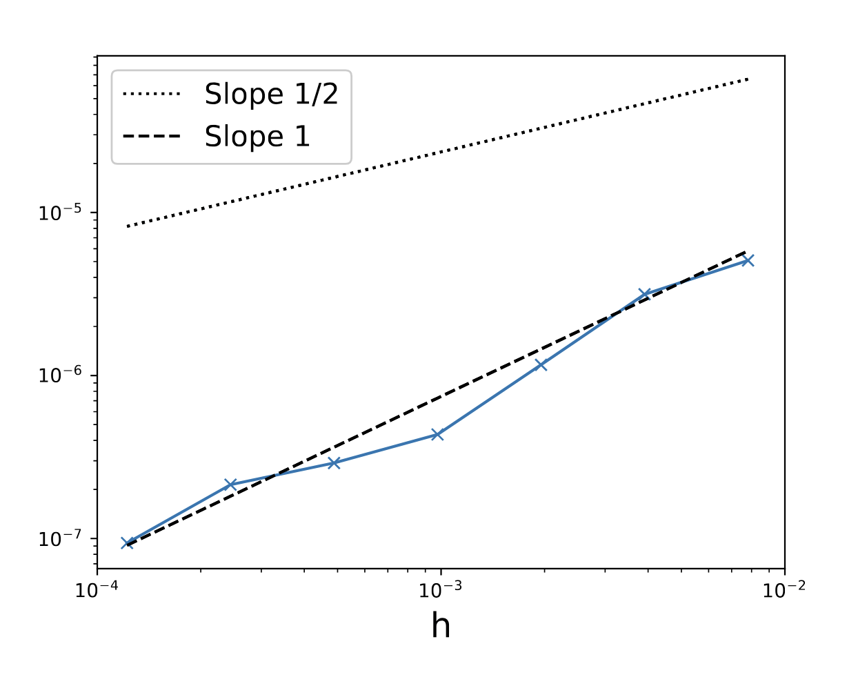
Mandatory error plots
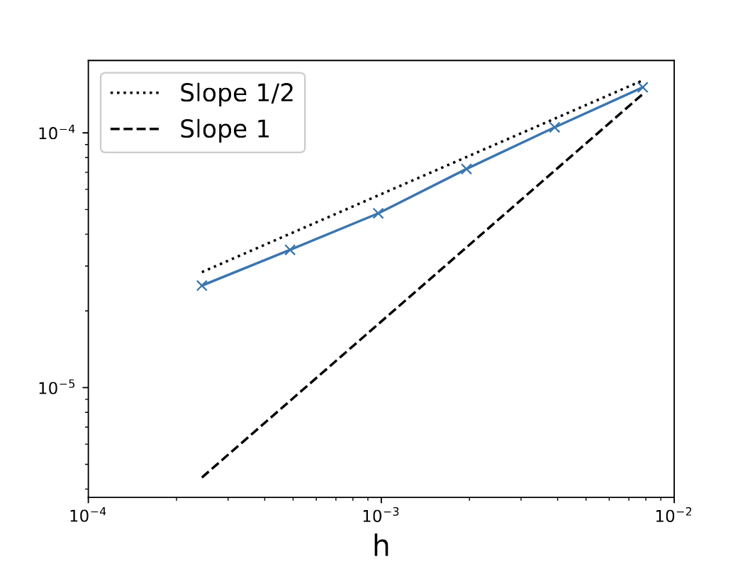
Strong error
Weak error
Rigid body
500 realizations
10^7 realizations
\(\phi(X) = \sin(2\pi x_1) + \sin(2\pi x_2) + \sin(2\pi x_3)\).
What's all this for?
Zeitlin is a convenient computational method for 2D ideal spherical hydrodynamics.
What's all this for?
Matrices are very large, makes exponential map/algebra to group mappings too expensive.
What's all this for?