Geometric shape matching for single-particle Cryo-EM data

slides.com/erikjansson
Joint work with:
- Klas Modin (Chalmers/University of Gothenburg)
- Ozan Öktem (Royal Institute of Technology, Stockholm)
- Jonathan Krook (Royal Institute of Technology, Stockholm)
Talk based on:
asdasdasd

But what is a shape?
Shape analysis


Point cloud on torus
Function on \([0,1]^2\)
Density on \([0,1]\)
Anything a diffeomorphism can act on!
What is a shape?
A warp is determined by a time-dependent vector field \(v\)
A vector field generates a curve of diffeomorphisms \(\gamma: [0,1] \mapsto G = \operatorname{Diff}(M)\) by
\(\dot \gamma(t) = \nu(t, \gamma(t)), t \in [0,1], \gamma(0) = \operatorname{Id} \)
The optimal vector field is a minimizer of an energy!
What is an optimal warp?
The energy functional
Canonical choice! Use right-invariant metric
The energy functional
Only depends on final value of \(\gamma(t)\)
Changes depending on application
The energy functional
Only depends on final value of \(\gamma(t)\)
Depends on whole path
Changes depending on application
Key question: How does \(\nu\) evolve?
(Answer: Use calculus of variations, but with which energy?)
The energy functional
Evolution of vector field does not care about matching!
Cannonball does not care about target
Shooting analogy
Use the Lagrangian \({\int_0^T \int_M L\nu(t) \cdot \nu(t)\mathrm{d}x\mathrm{d}t}_{}\)
Calculus of variations gives:
The EPDiff equation
Matching by shooting
A picture says more...

Shape analysis made simpler
The ingredients you really need:
A Lie group of deformations \(G\) acting on a set of shapes \(V\) (metric space)
Flexible choice
Right-invariant metric (not so flexible)
Shape: indirect matching
Here, \(A\) and \(B\) are assumed to be elements in the same space.
What if we cannot directly observe B?
Shape: indirect matching
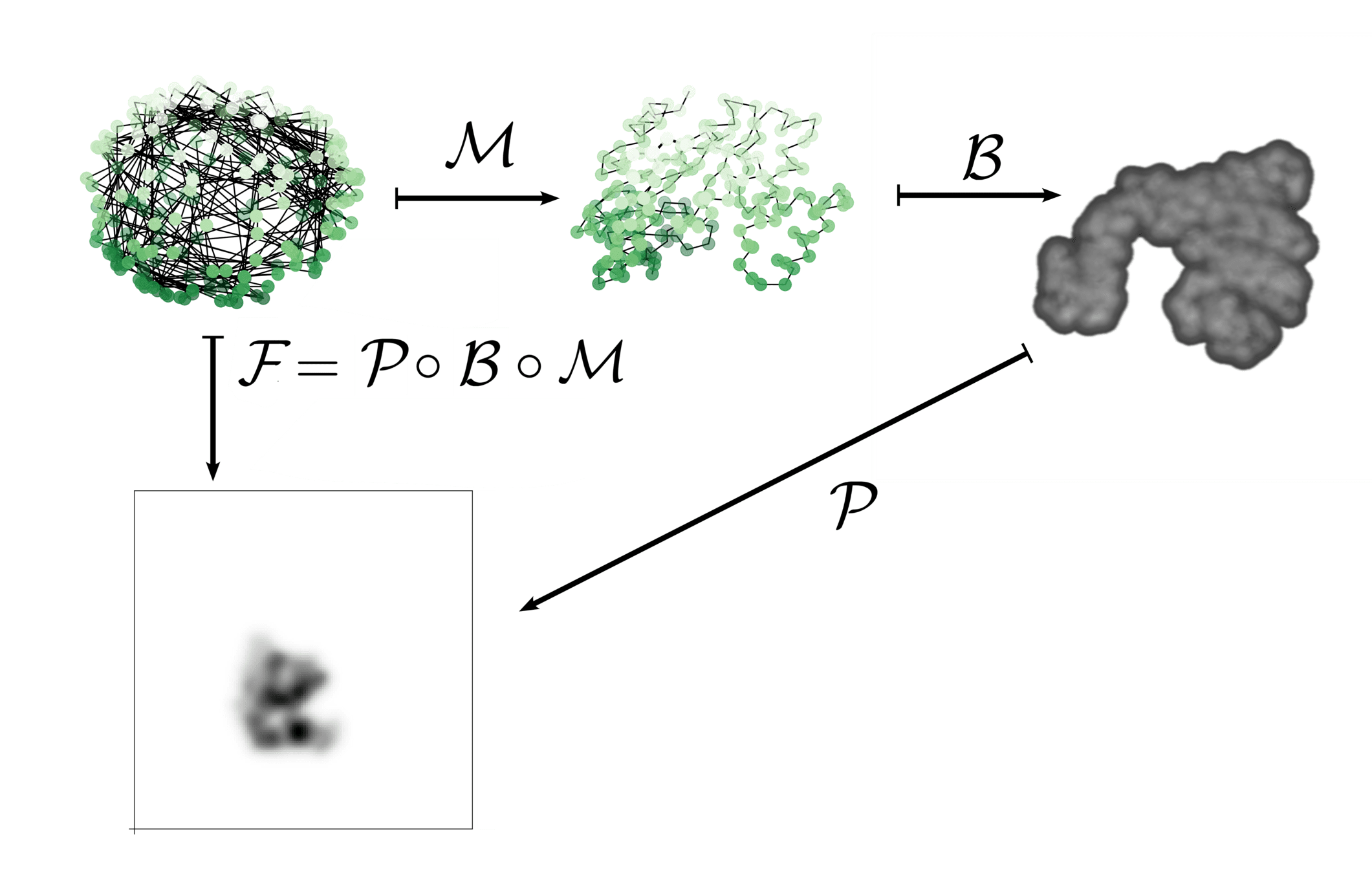
Include a forward operator \(\mathcal{F}\colon V \to W\)
Initial shape: \(A \in V\)
Target shape: \(B \in W\)
Doesn't affect mathematical framework!
"Reconstructs" the \(\gamma(1).A\) that best would map to \(B\)
Shape for Cryo-EM
Single-particle Homogeneous Cryo-EM in 30 seconds (by a maths person)
Electron
microscope

Low dose - low SnR
Many images
Shape for Cryo-EM
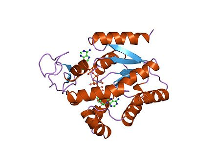
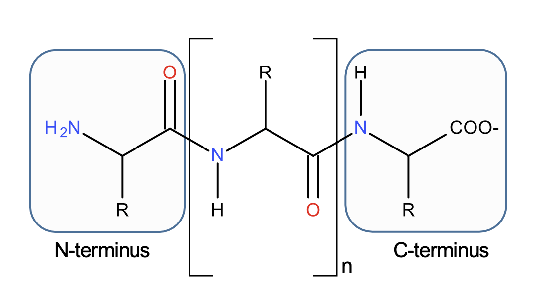
Proteins in 30 seconds (by a mathematician)
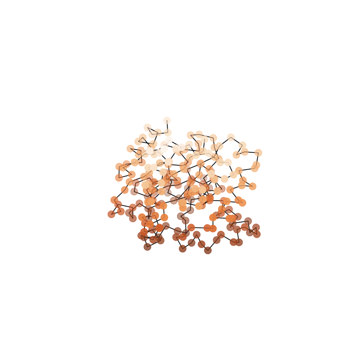
In this work: forget about everything but the \(C_\alpha\)s
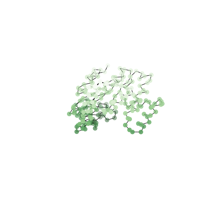
Relative positions
Shape for Cryo-EM
Shape space: space of relative positions \(V = \mathbb{R}^{3N}\)
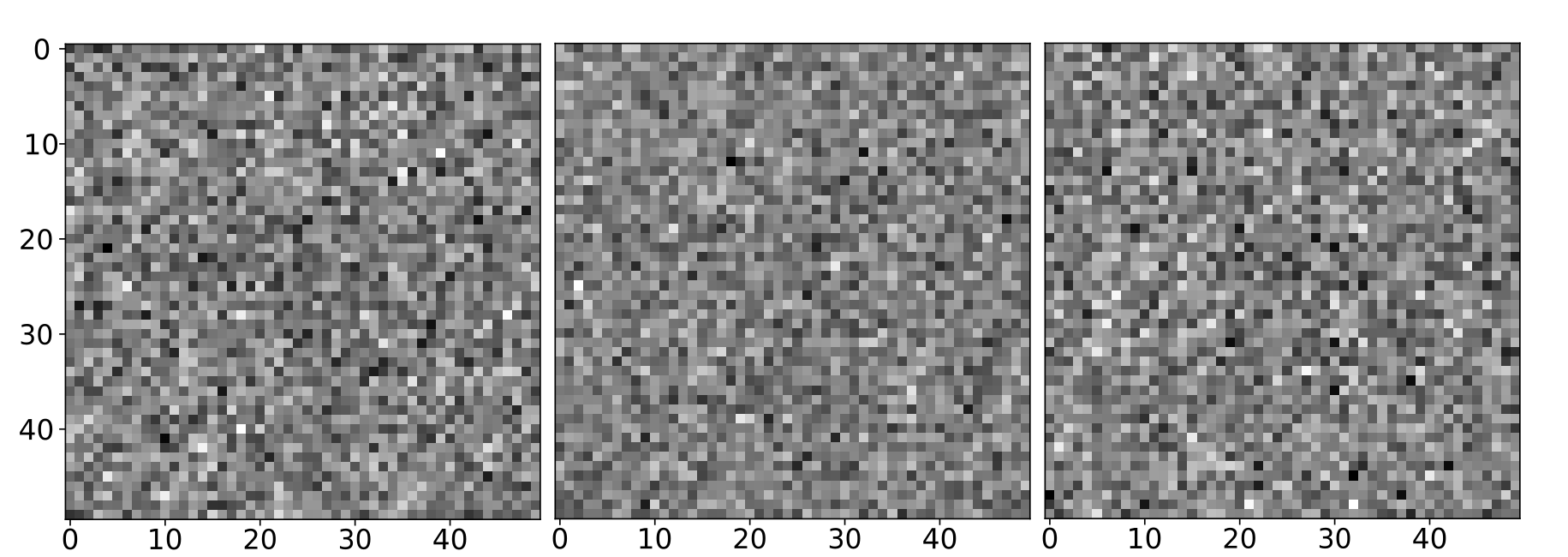
Data space - 2D images, \(L^2(\mathbb{R}^2)\) (very noisy!)
However: We want rigid deformations, so \(G = \operatorname{SO}(3)^N\), and \(\operatorname{dim}(G) \ll \operatorname{dim}(\operatorname{Diff}(M)) = \infty\)
Todo: Construct forward model, decide on energy, compute gradients, set up optimization routine
Shape for Cryo-EM
Forward model building
Shape for Cryo-EM
Forward model building
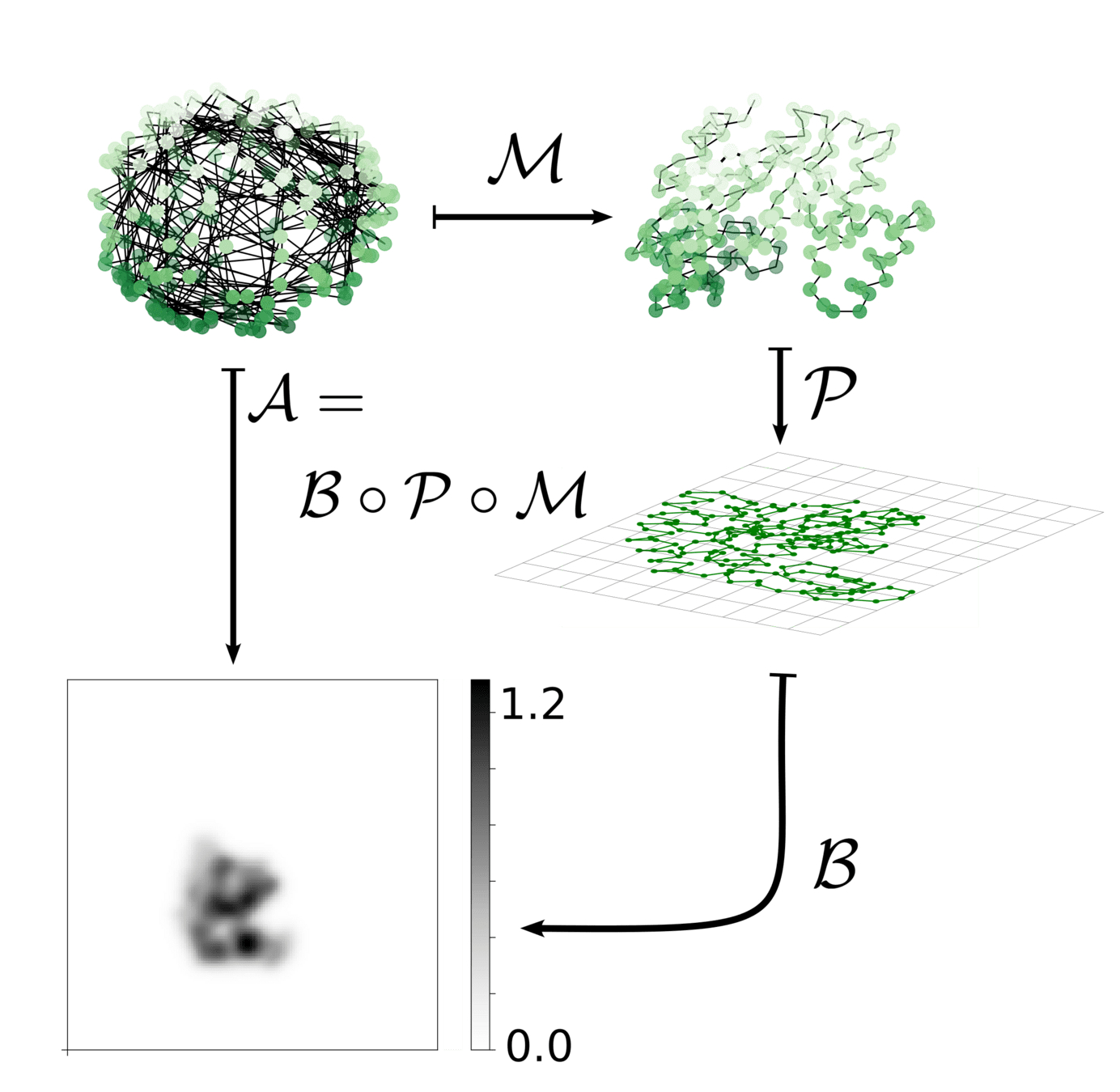
Shape for Cryo-EM
Similarity score is clear. For now: use x-y-z projections (3 images)
Shape for Cryo-EM
Similarity score is clear. For now: use x-y-z projections (3 images)
- Guess \(\nu(0)\) (or path sampled at discrete points)
- Integrate
- Evaluate \(\mathcal{E}\) and compute \(\nabla_{\nu(0)} \mathcal{E}\)
- Update \(\nu(0)\) with favorite algorithm (A few GD steps and then L-BFGS-B)
Gradient is available (even easy to compute)
(but ugly)
Shape for Cryo-EM
Gradient is available
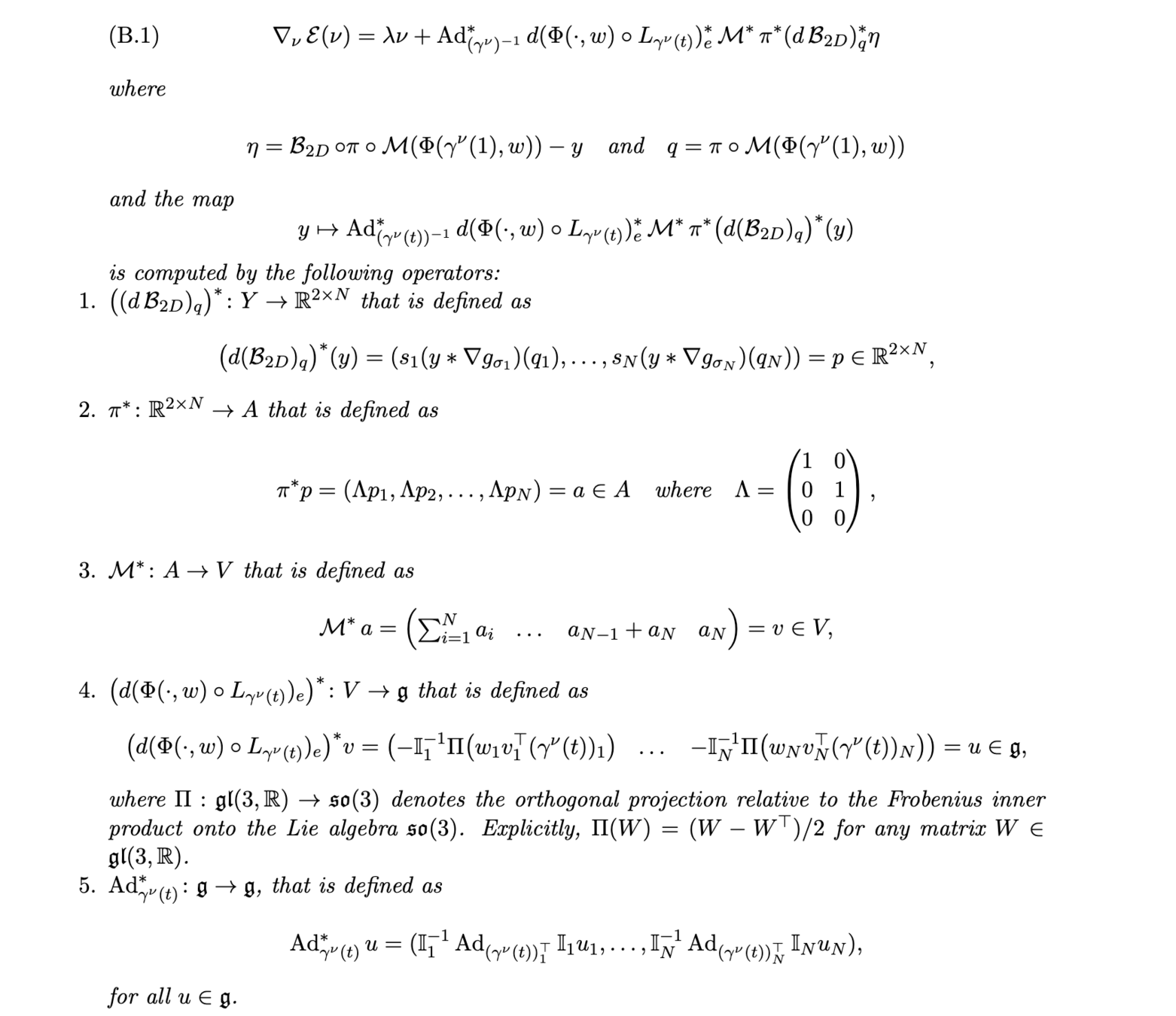
Shape for Cryo-EM
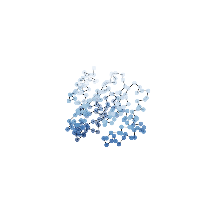
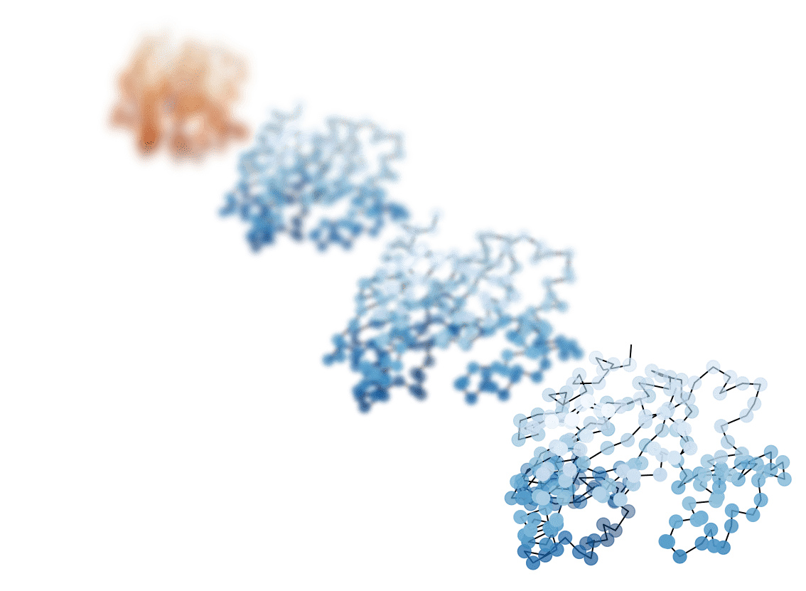
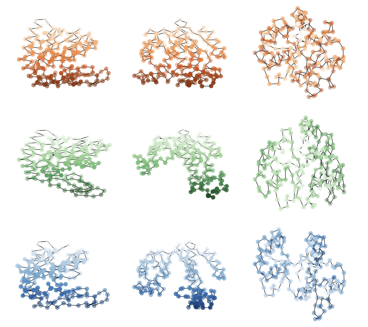
Deformation
What we want
What we see
Where we start
Shape for Cryo-EM
Oh no
but....
Shape for Cryo-EM
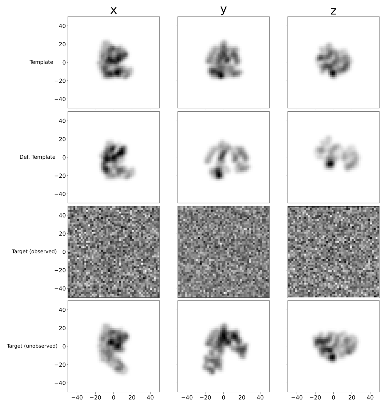
x
y
z
Deformed
Target
Template
Shape for Cryo-EM
Shape for Cryo-EM
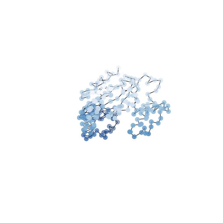
Hope!
Turn up number of images used
Decent in the directions we have projections
Shape for Cryo-EM
Deformation
What we want
What we see
Where we start
Shape for Cryo-EM
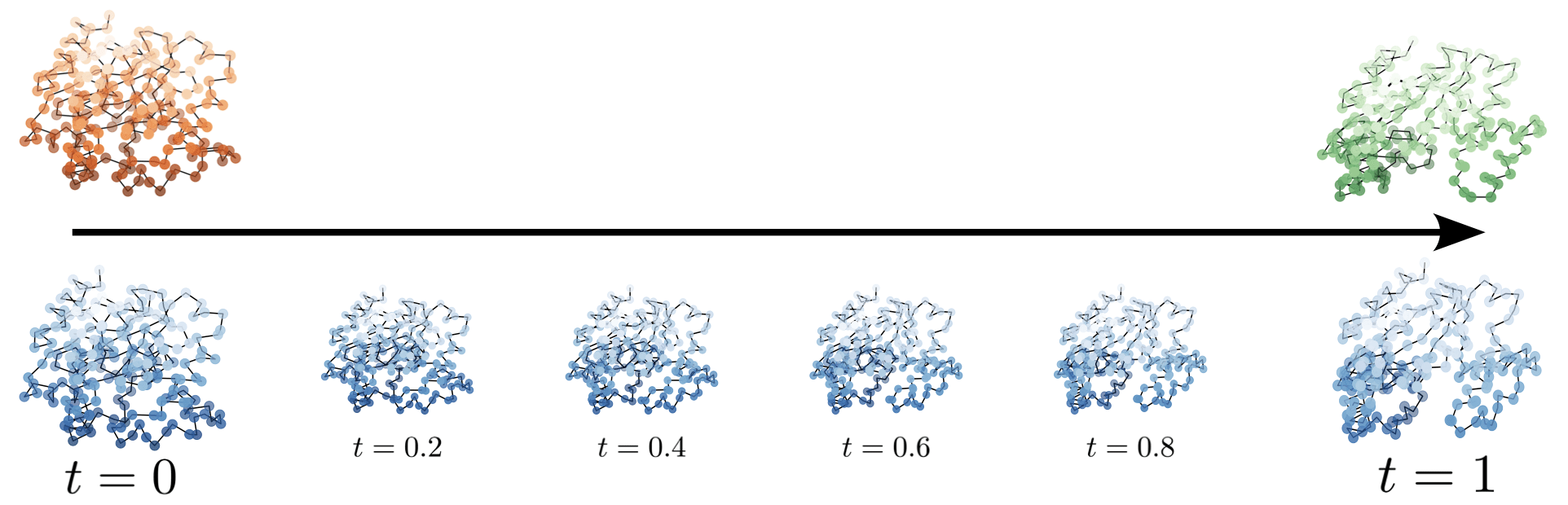
Deformation path
Note: Deformation makes no physical sense
Shape for Cryo-EM
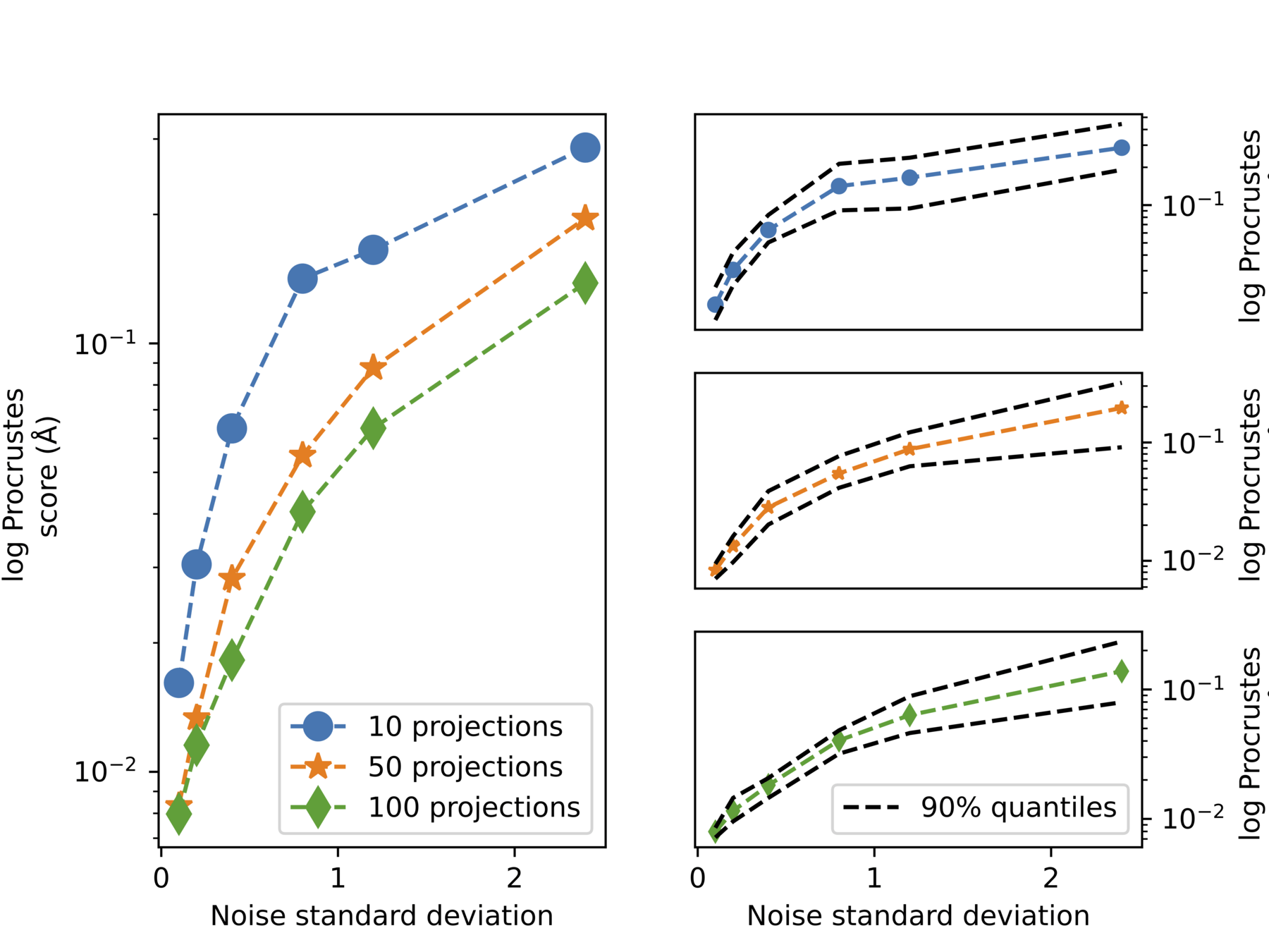
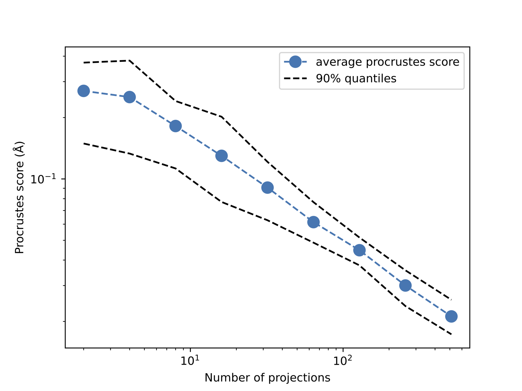
Increase noise
Increase #projections
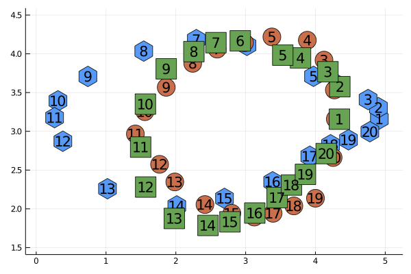
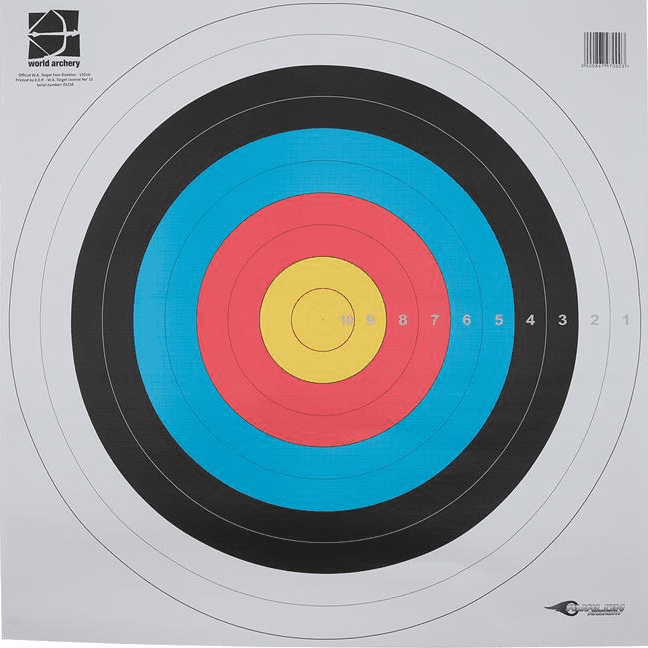
Quantative measure: Procrustes score
Procrustes analysis
Two point clouds \(\mathbf x = (x_i)_{i=1}^K\) and \(\mathbf y = (y_i)_{i=1}^K\)
Rotate, reflect, scale and translate ("superimpose") \(\mathbf x\) to be as close in mean-square sense to \(\mathbf y\) as possible
As close as we can get: Procrustes distance (early statistical shape analysis measure)
In conclusion: Early days...
- Global pose: We assume it is known
- Side chains: We cut away the side chains
- Faster methods: Even if we have the gradient, not fast!
Shape analysis seems promising