Geometric numerical methods: from random fields to shape matching
Geometric numerical methods: from random fields to shape matching
Geometric numerics?
Numerical analysis: the art of being wrong in the mathematically correct way
Concerned with the approximate solution of continuous problems
Geometry: the study of space: distance, shape, size, angles...
Geometric numerics: How to approximate solutions to geometric problems

Shape analysis and matching problems
Structure-preserving numerics for geometric mechanics
Elliptic SPDEs on manifolds
for sampling of random fields
GEOMETRIC
NUMERICAL
METHODS
Random fields via stochastic partial differential equations
Paper I and II research questions
What is a random field?
Definition: Stochastic process indexed by spatial domain: Assigns random value to each point on domain
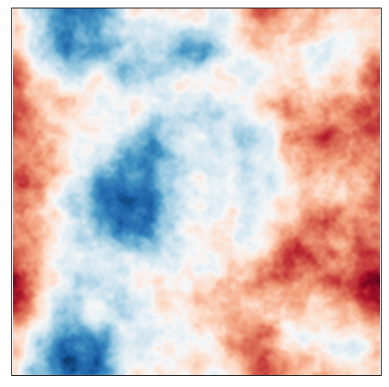
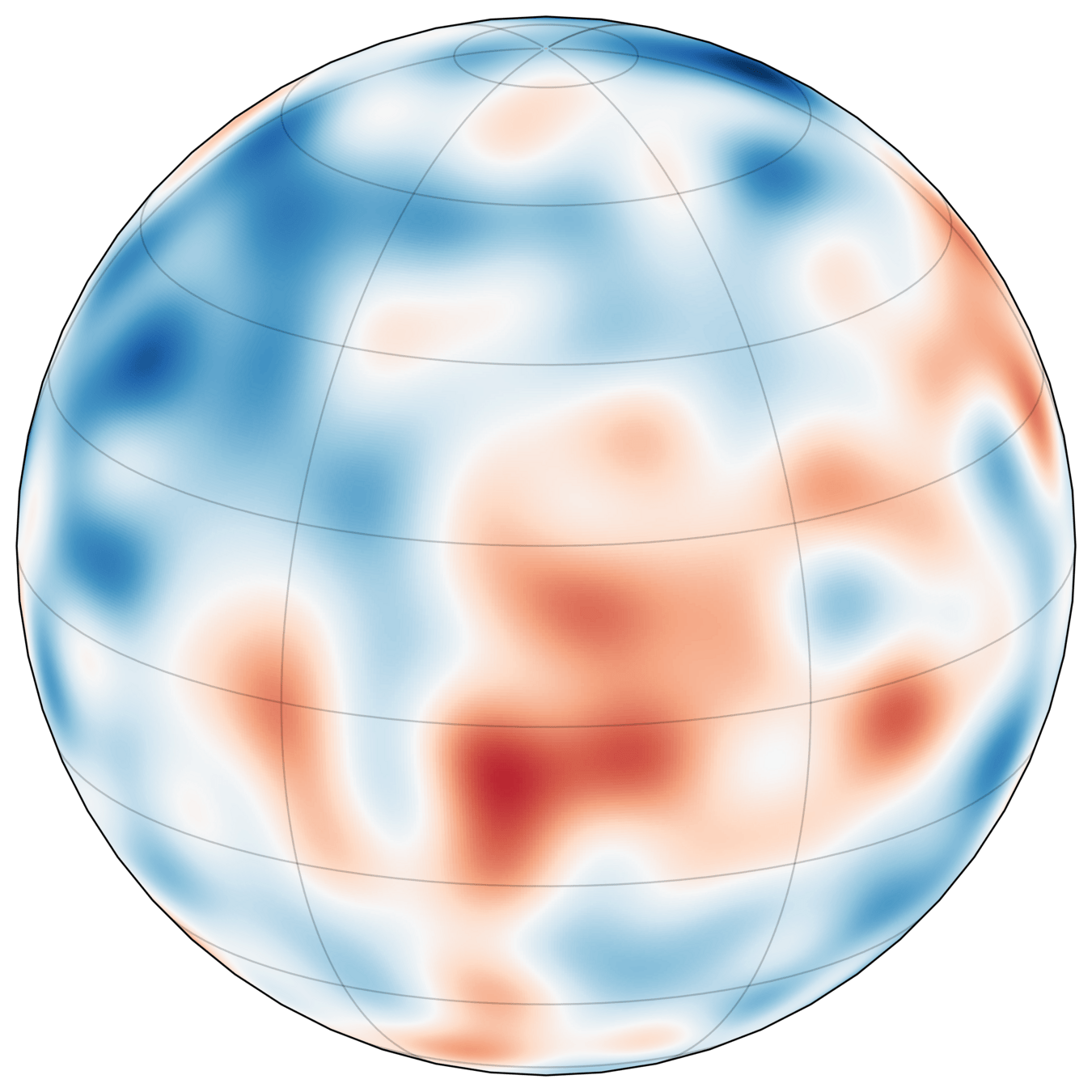
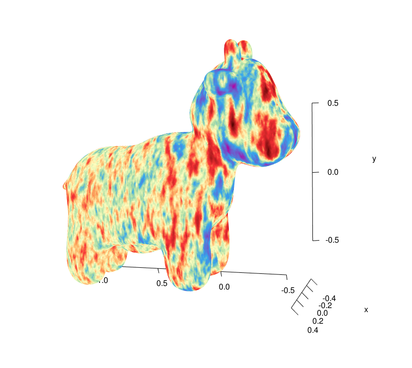
We consider Gaussian random fields on surfaces generated by coloring white noise with linear operators that are functions of differential operators.
Our models
Classical model inspired by the commonly used Matérn kernel. Whittle–Matérn fields.
Novel, more flexible model proposed by us
Contains Whittle–Matérn fields.
Research questions and approaches
Statistics phrasing: How to sample the fields?
Numerics phrasing: How to approximately solve for \(\mathcal Z\)
Two approaches
Paper I
Paper II
- Restricted to sphere
- Approximate fractional part with quadrature
- Solve family of systems recursively with FEM
Main scientific question: Convergence of method
- Hypersurfaces in \(d = 2,3\)
- Approximate white noise on FEM space
- Color approximated white noise with projected operators
Both fundamentally based on surface FEM methods
Main scientific question: Convergence of method
Shape analysis
and matching problems
paper IV and VI research questions
Shape analysis
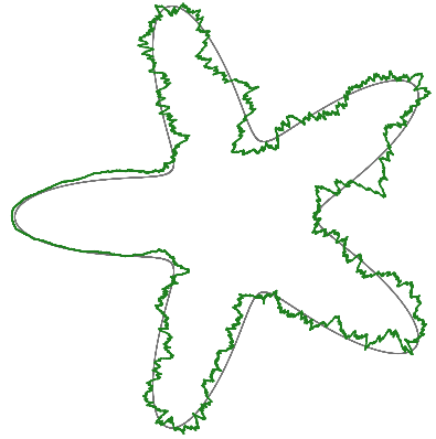
But what is a shape?
But what is a shape?
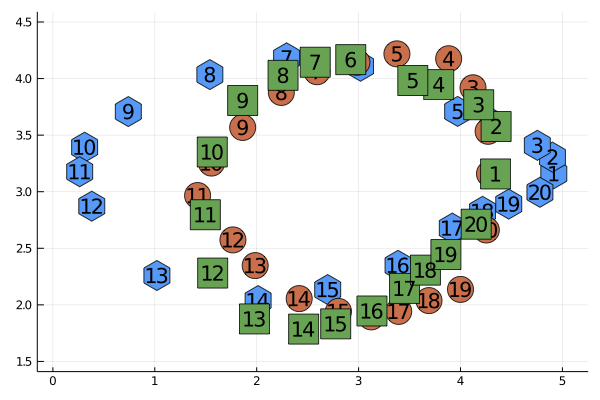

Point cloud on torus
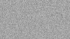
Function on \([0,1]^2\)
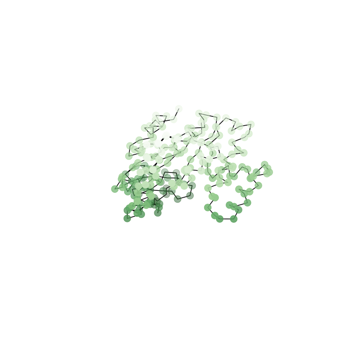
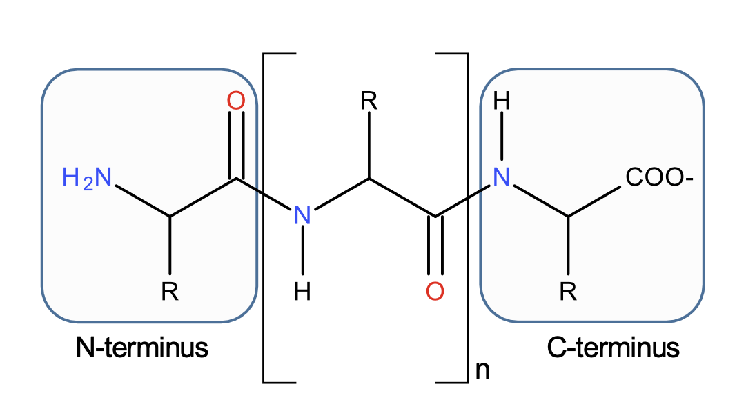
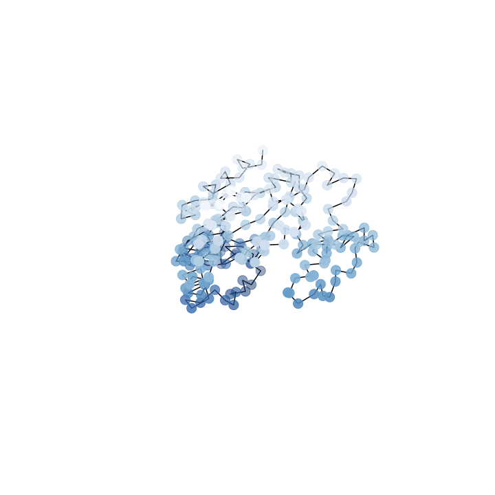
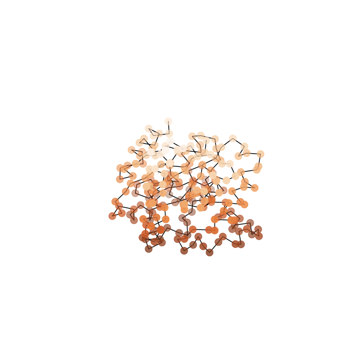
A protein backbone
Shapes are in a (metric) space \(V\) acted upon by a Lie group of deformations \(G\).
\(V = (\mathbb{T}^2)^N\),
\(G = \operatorname{Diff}(\mathbb{T}^2)\)
\(V = C^\infty([0,1]^2)\),
\(G = \operatorname{Diff}([0,1]^2)\)
\(V = \mathbb{R}^{3N}\),
\(G = \operatorname{SO}(3)^N\)
Matching is an optimization problem
Deformations \(g\) is endpoint of curve \(\gamma \colon [0,1] \to G \)
Right-invariance of metric
In thesis: indirect matching
What if \(A\) and \(B\) are not in the same space?
Application: Indirect observation of B?
Indirect matching
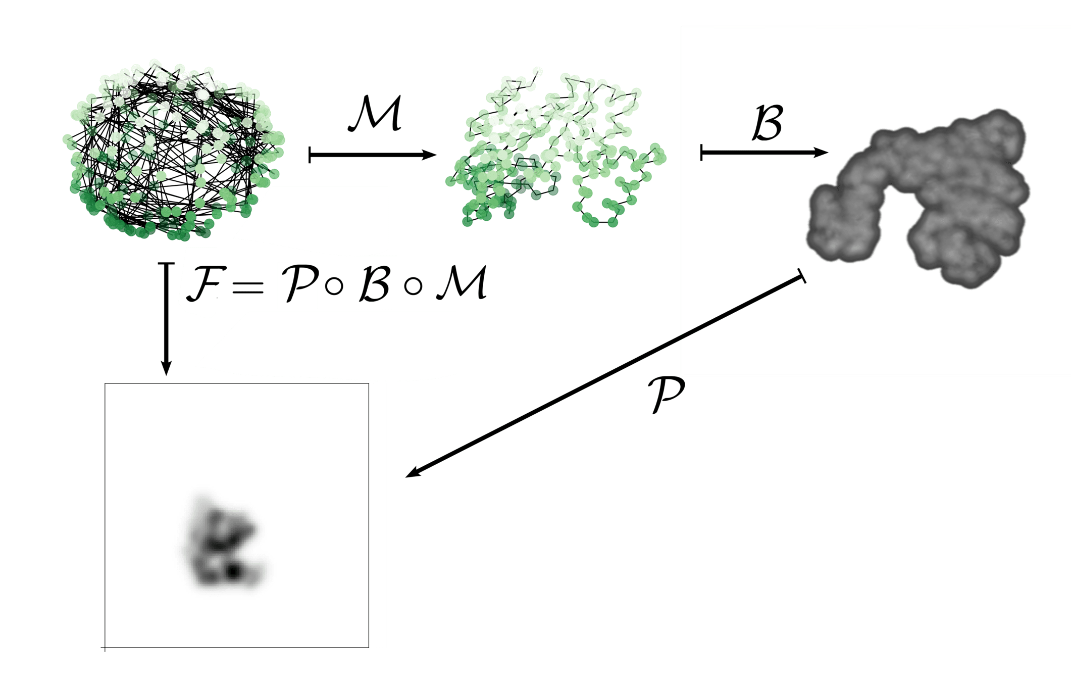
Include a forward operator \(\mathcal{F}\colon V \to W\)
Initial shape: \(A \in V\), target shape: \(B \in W\)
"Reconstructs" the \(\gamma(1).A\) that best would map to \(B\)
Research questions and approaches
Paper IV
Paper VI
Constrain landmarks to move only in certain directions
The reconstruction of protein confirmations is difficult.
Applications cases of (indirect) shape matching
- Shapes are landmarks
- Deformation group is diffeomorphism group
- Possible indirect matching against labels
- Shapes are protein backbones
- Deformation group is a matrix group
- Indirect matching against noisy cryo-EM images
Main scientific question:
Can constrained landmark matching be seen as a neural net?
Main scientific question:
Is indirect shape matching a viable approach for protein conformation reconstruction?
Structure-preserving numerics for geometric mechanics
Paper III and VII research questions
Mechanical problems
Focus here: Lie–Poisson systems: Related to the evolution of observables in Hamiltonian mechanics
Evolves on dual of Lie algebra \(\mathfrak{g}^*\)
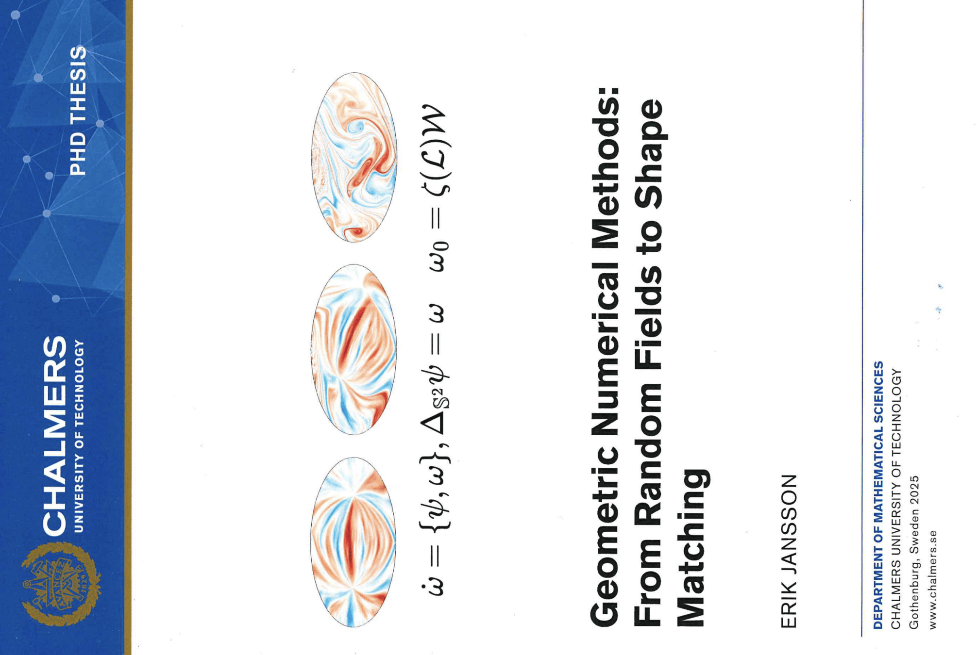
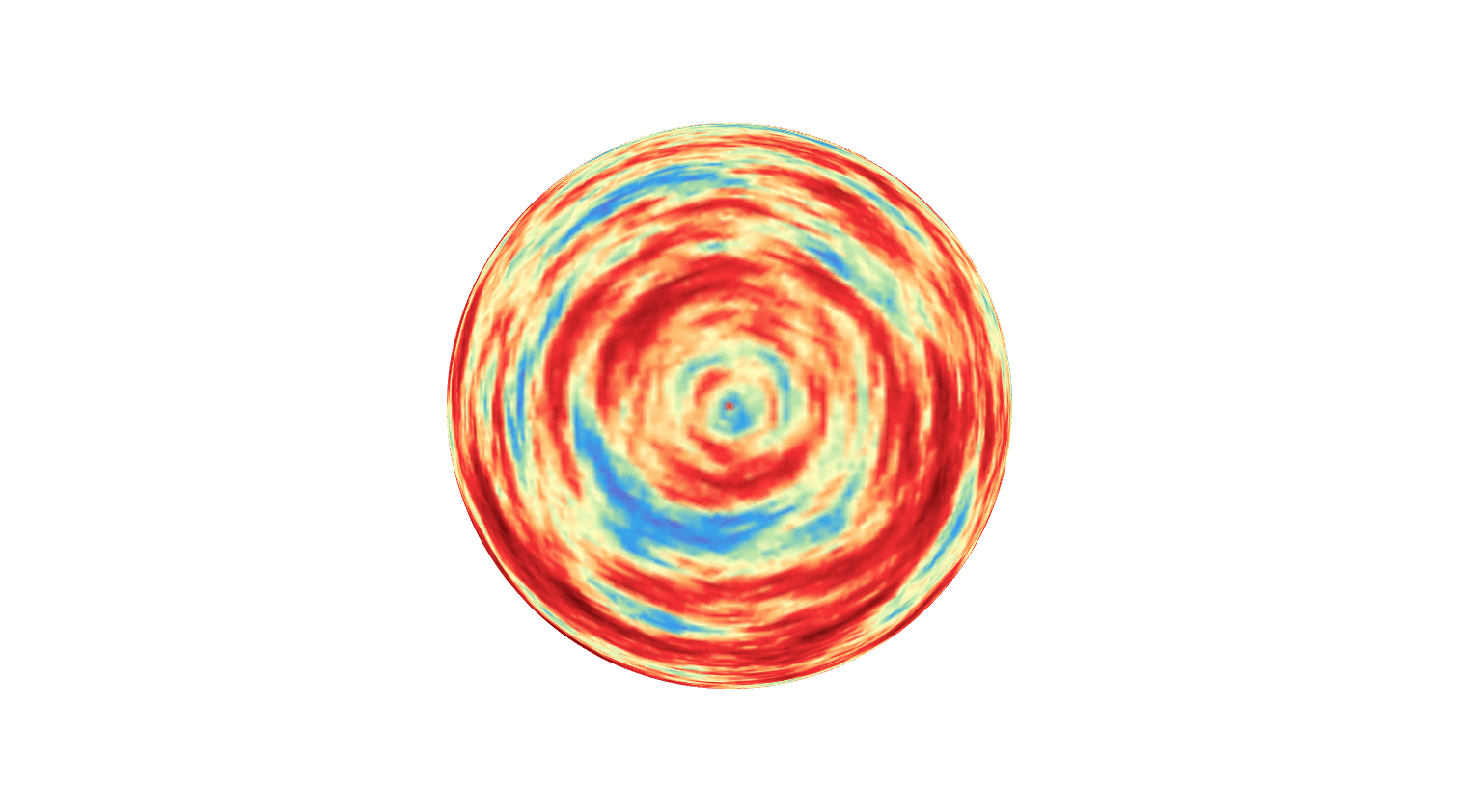
Complexified Euler equations:
Rigid body equations:
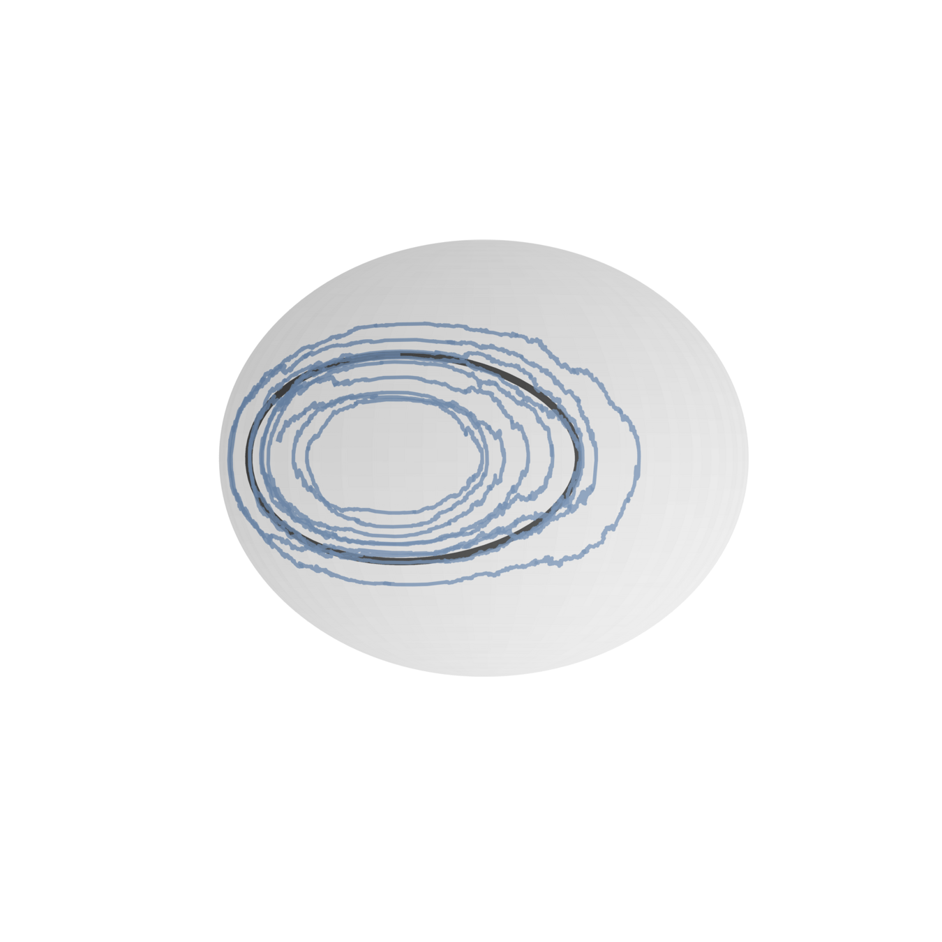
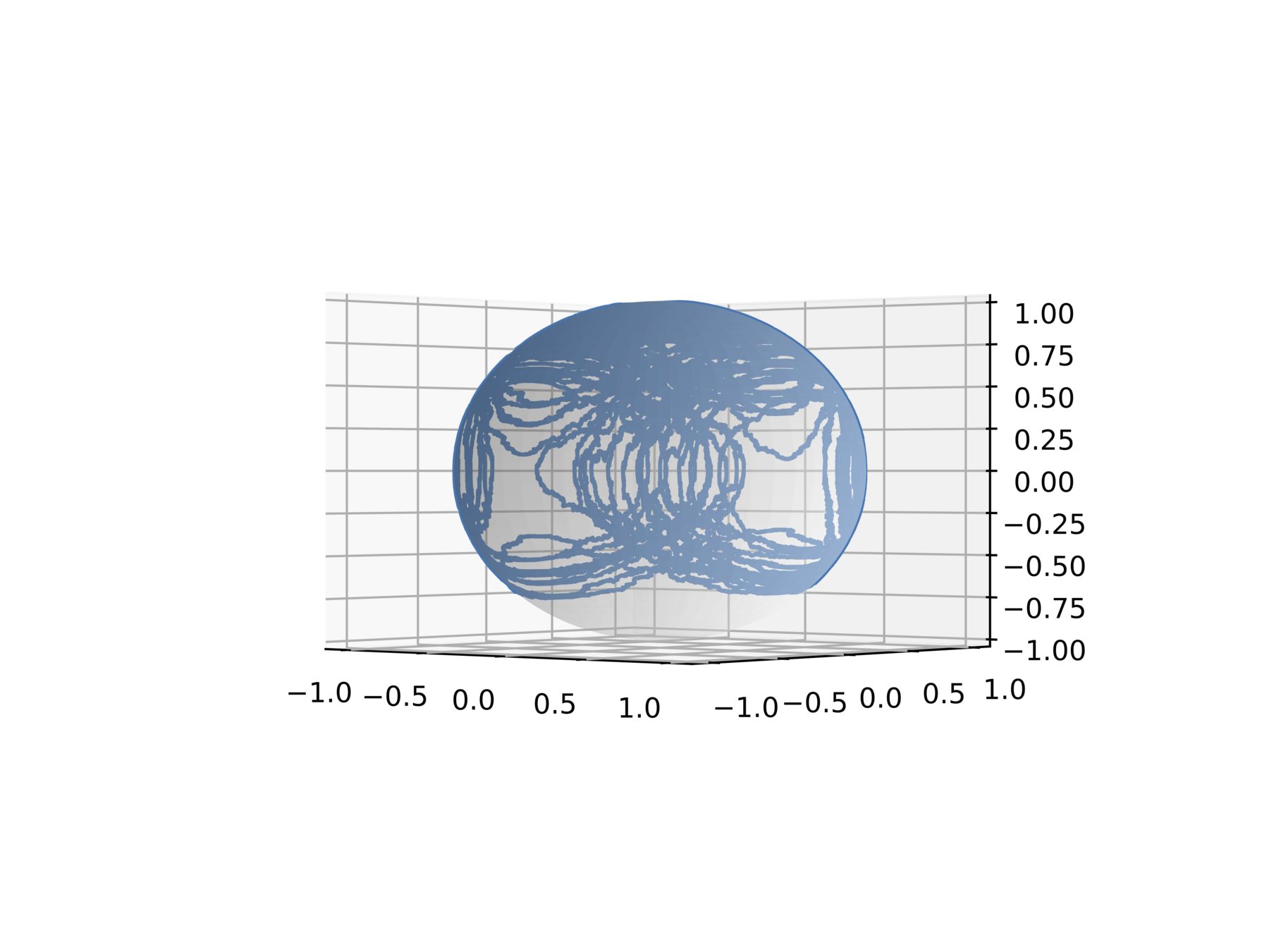
Geometry of LP systems
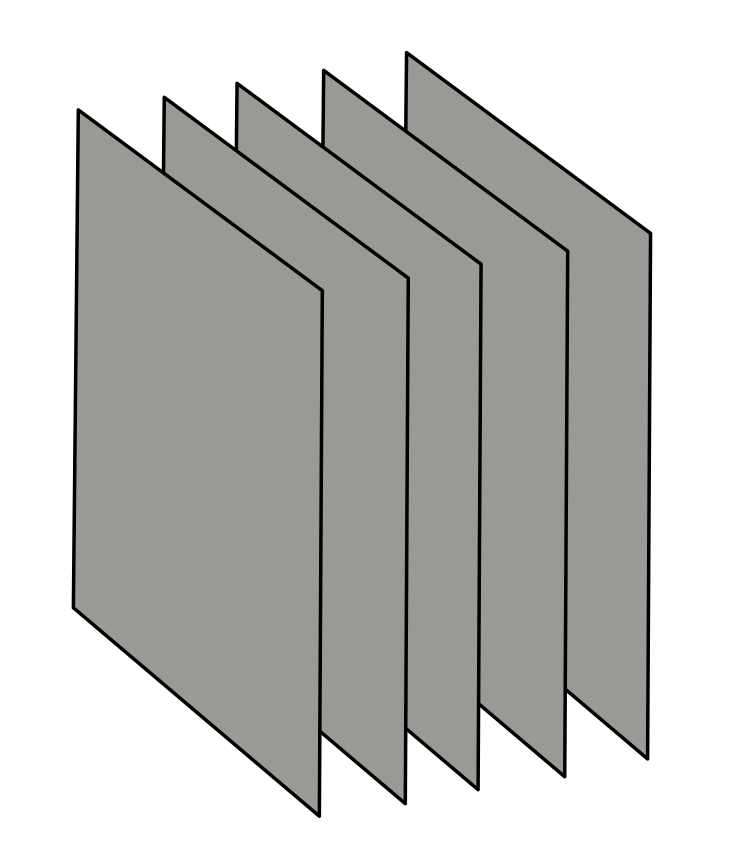
LP system has a rigid geometric structure:
they evolve on coadjoint orbits
In addition: conserved quantites
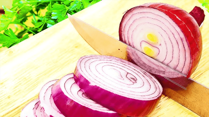
They look like onions, sometimes
Discretizations in time for ODEs and time and space for PDEs with LP structure should respect LP structure and conserved quantities
Research questions and approaches
Paper III
Paper VII
- Stochastic Lie–Poisson systems in high but finite dimensions
- Existing geometric integrators can be expensive if dimension is large
- Deterministic case: IsoMP method
- Can we develop a stochastic IsoMP method?
Main scientific question: Development, analysis and convergence of method
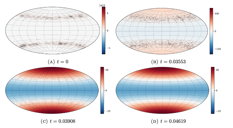
- Complexified Euler equations on \(\mathbb T^2\) are ill-posed (blow-up)
- Zeitlin's method + IsoMP provides an LP-preserving numerical method
- Blow-up is inherently at limit of numerics, what is a reliable signature?
Main scientific question: How to detect blow-up with geometric numerics?
Scientific questions: recap
- What is convergence behavior analysis of our methods for SFEM-based simulation approach of random fields?
- What is the behavior of our stochastic IsoMP method?
- What is a reliable numerical signature of blow-up?
- What is the connection between constrained landmark matching and neural networks?
- Does shape analysis have a future in protein imaging?
Thesis research
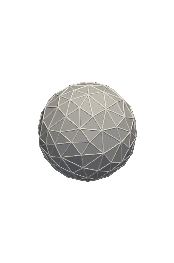
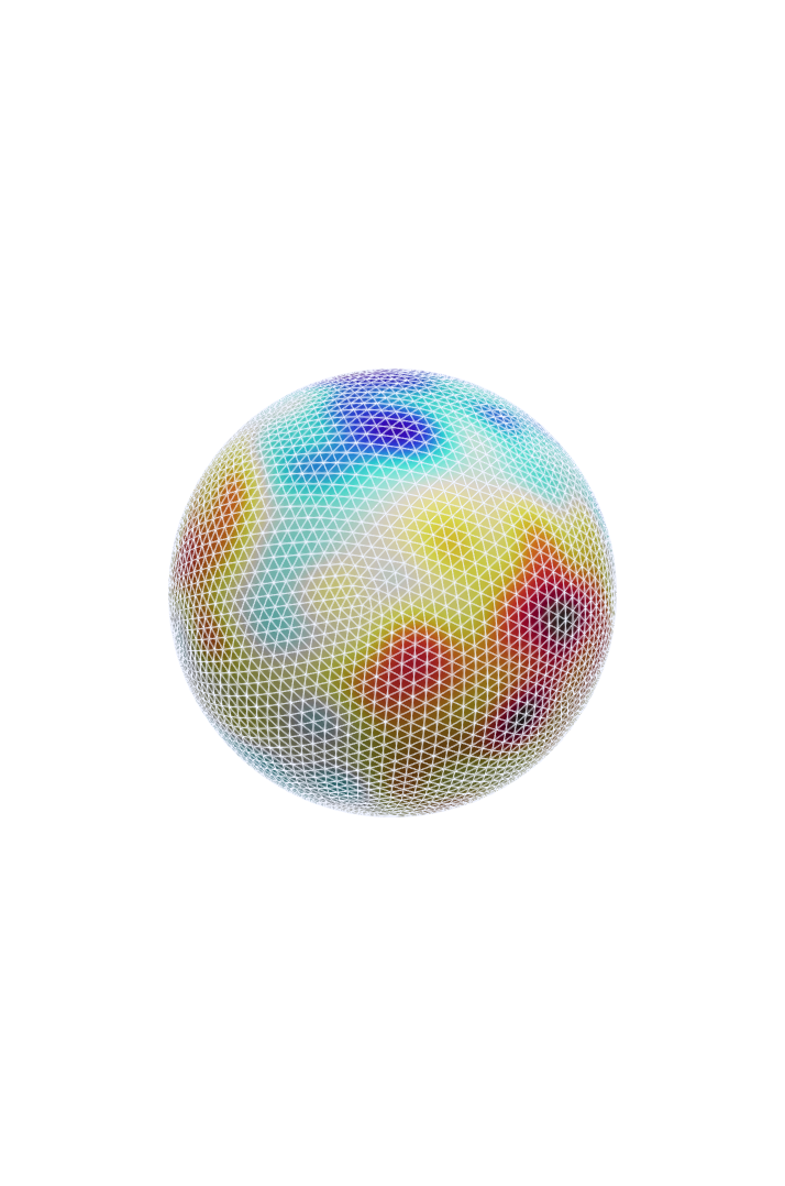
Paper I: Generate random fields of well-known type on the sphere by SPDE and SFEM approach.
Paper II: Generate random fields of new type by coloring approximated white noise
Paper III: Development of structure-preserving integration of stochastic Lie–Poisson systems
Paper VII: Trustworthy structure preserving numerics for blow-up detection
Paper IV: Sub–Riemannian landmark matching and connections to neural networks
Paper V: Convergence analysis of a gradient flow
Paper VI: Indirect shape matching for protein conformation reconstruction
Thesis research
Paper I: Generate random fields of well-known type on the sphere by SPDE and SFEM approach.
Paper II: Generate random fields of new type by coloring approximated white noise
Paper IV: Sub–Riemannian landmark matching and connections to neural networks
Paper V: Convergence analysis of a gradient flow
Paper VI: Indirect shape matching for protein conformation reconstruction
Paper III: Development of structure-preserving integration of stochastic Lie–Poisson systems
Paper VII: Trustworthy structure preserving numerics for blow-up detection
Main findings
Paper II: Strong error rates for the algorithms proven using functional calculus approach
Paper III: IsoMP is made stochastic. Method is analyzed by using the geometric structure of LP systems.
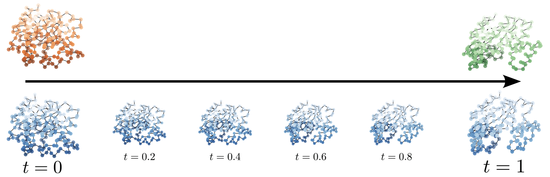
Paper VI: Shape matching is adapted to the protein conformation reconstruction setting and is showcased as a promising approach
Random fields via stochastic partial differential equations
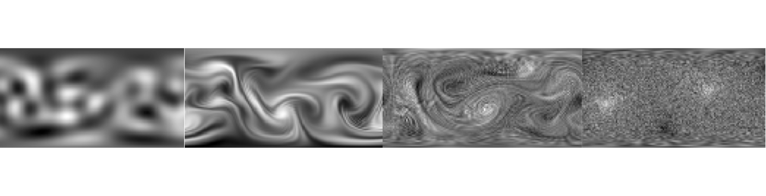
Paper II results
Some more details on paper II
Our approach is best understood by spectral expansions.
Eigenpairs of \( \mathcal{L} \): \((\lambda_i,e_i)\)
Field approximation using eigenpairs \((\Lambda_{i,h},E_{i,h})\) of \(\mathsf L_h\)

Geometry
approximation
Our method
In practice:
Key benefit:
Find a mesh and you can simulate GRFs on it! No need to know the geodesic distance
Research question: Strong error?
\((Z_i)\) are Gaussian with covariance matrix determined by \(\zeta\) and FEM matrices
Resolving research question
Key method:
Shape analysis
and matching problems
Paper VI results
Cryo-EM
in 30 seconds (by a maths person)
Electron
microscope

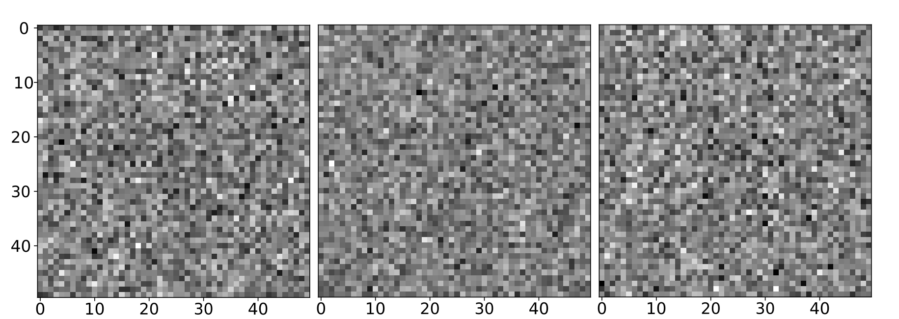
Low dose - low SnR
Many images
Many copies of the same protein but at different orientations and conformations
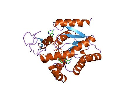
Proteins in 30 seconds (by a mathematician)
In this work: forget about everything but the \(C_\alpha\)s
Relative positions
\((\mathbb R^3)^N\)
Mathematical model for proteins
Proteins: mathematical model
Idea: Take a known conformation of the protein as a "prior"
Deform it until it matches target
How to deform? And what energy to use?
Optimization problem!
Shape for Cryo-EM
Shape space: space of relative positions \(V = \mathbb{R}^{3N}\)
Data space - 2D images, \(L^2(\mathbb{R}^2)\) (very noisy!)
We want rigid deformations, so \(G = \operatorname{SO}(3)^N\)
Forward model
Shape for Cryo-EM
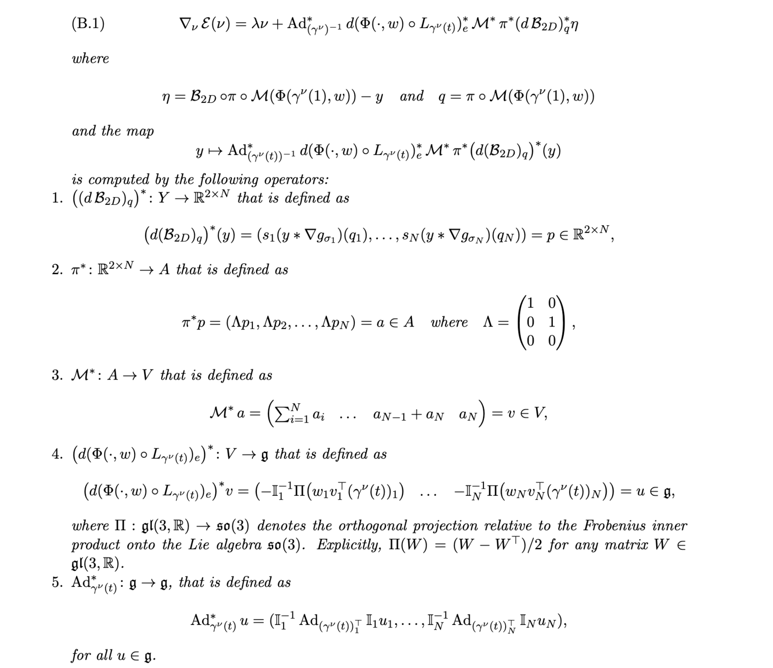
Minimization of \(\mathcal E(\nu) \) reduces to:
+ shooting
Shape for Cryo-EM
- Guess \(\nu(0)\) (or path sampled at discrete points)
- Integrate to get \(\gamma(1)\)
- Evaluate \(\mathcal{E}\) and compute \(\nabla_{\nu(0)} \mathcal{E}\)
- Update \(\nu(0)\) with favorite algorithm (A few GD steps and then L-BFGS-B)
Gradient is available (even easy to compute)
Shape for Cryo-EM
Deformation
What we want
What we see
Where we start
Research question: It's looking viable
Results using shape framework
Structure-preserving numerics for geometric mechanics
Paper III results
- \(M\) independent scalar Brownian motions \(W^1, \ldots, W^M\)
- \(M\) noise Hamiltonians \(H_k\colon\mathfrak{g}^*\to \R\)
Stochastic LP systems
LP systems on \(\mathfrak{g}^*\), stochastic or not, are reductions of Hamiltonian systems on \(T^*G \cong G \times \mathfrak{g}^*\)
There is a mapping \(\mu\) that takes LP system to a left-invariant Hamiltonian system (reconstruction)
Stochastic LP systems

upstairs
downstairs
Stochastic Hamiltonian system:
know how to numerically integrate.
Properties of method known
Stochastic Lie–Poisson system:
Don't know how to integrate
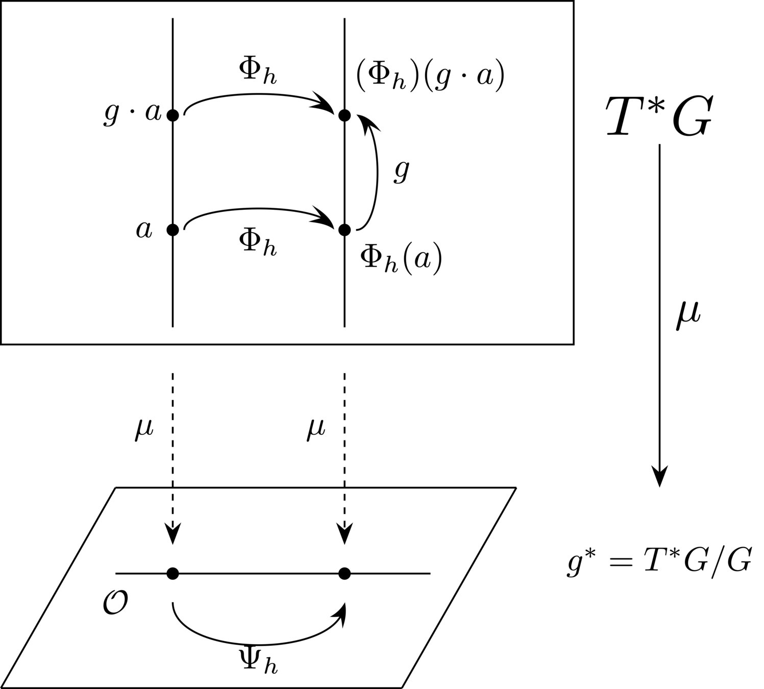
Idea: make sure the "stairs" \(\mu\) has nice properties and takes integrator upstairs to integrator downstairs
Intuitive picture:
\(\Phi_h \colon T^*G \to T^* G\): \(G\)-equivariant symplectic integrator \(\rightarrow\)
Reduces to a Lie–Poisson integrator by \(\mu\)
Use Implicit midpoint
Integration without tears
Exploit the reconstruction!
Error analysis without tears
Check the literature for error analysis for implicit midpoint
Exploit the reconstruction!
Result
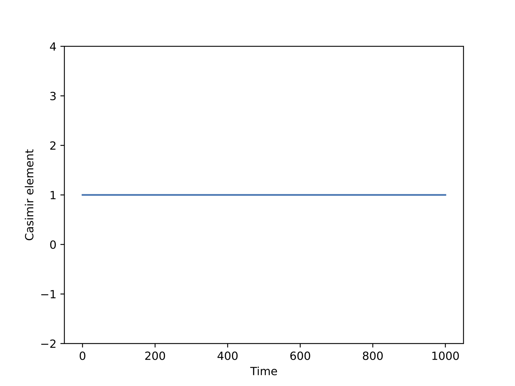
- Method is Lie–Poisson (preserves LP structure) surely
Scientific question is resolved
Scientific questions: conclusion
- What is convergence behavior analysis of our methods for SFEM-based simulation approach of random fields? Resolved in paper I and II
- What is the behavior of the stochastic IsoMP method? Resolved in paper III
- What is a reliable numerical signature of blow-up? Suggestion in paper VII
- What is the connection between constrained landmark matching and neural networks? One possible connection is studied in paper IV
- Does shape analysis have a future in protein imaging? Results in paper VI suggests it.
Outlook (if I had one more year)
Idea I: Extend to spatio-temporal fields
Idea II: Compute weak errors
Idea III: Stationarity on general manifolds
Idea IV: Regularization by noise in structure-preserving simulations
Idea V: Blow-up for axisymmetric 3D Euler with Zeitlin
Idea VI: GNNs for better fidelity terms in protein matching for more realistic behavior
Idea VII: Side chain inclusion
Idea VIII: Indirect shape matching via gradient flows
Paper I: Surface finite element approximation of spherical Whittle-Matérn Gaussian random fields. With Annika Lang and Mihály Kovács
Paper II: Non-stationary Gaussian random fields on hypersurfaces: Sampling and strong error analysis. With Annika Lang and Mike Pereira
Thesis research: coauthors
Paper III: An exponential map free implicit midpoint method for stochastic Lie-Poisson systems. Joint with Annika Lang, Sagy Ephrati and Erwin Luesink
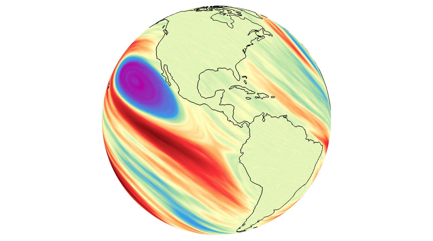
Paper VII: On spectral scaling laws for averaged turbulence on the sphere. Joint with Klas Modin
Paper IV: Sub-Riemannian landmark matching and its interpretation as residual neural networks. With Klas Modin
Paper V: Convergence of the vertical gradient flow for the Gaussian Monge problem. With Klas Modin
Paper VI: Geometric shape matching for recovering protein conformations from single-particle Cryo-EM data. With Ozan Öktem, Jonathan Krook and Klas Modin
Extra slides: Paper I
Details of methods and proof
Error
EXTRA: Special case: sphere
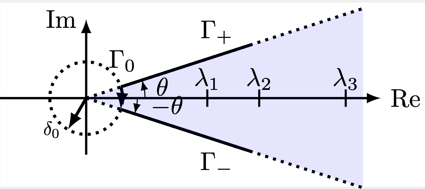
Main difference: the fractional part is approximated by a Dunford–Taylor integral sinc quadrature!
Split problems to obtain recursion!
\(\|u-u_{Q,k}\|\) decays exponentially in \(k\)
EXTRA: Special case: sphere
In general
The error from the geometry discretization is the error of the previous problem in the recursion!
EXTRA: Special case: sphere
EXTRA: Special case: sphere
Extra slides: stationarity of RFs on surfaces
G-homogeneous spaces
G-iostropic fields
Geodesic stationarity
Counterexample
EXTRA: Stationarity/isotropic
\(G\) is a Lie group. Let \(M\) be a G-homogeneous space.
\(G\) acts transitively on \(M\):
For all \(x,y \in M\) there is a \(g \in G\) so that \(g\cdot x = y \)
Examples:
- \(\operatorname{SE}(d)\) and \(\mathbb{R}^d\)
- \(\operatorname{SO}(d)\) and \(\mathbb{S}^d\)
- Orthogonal group and Stiefel manifold
Stationarity = probabilistic invariance under action of group.
Consequence: covariance function depends only on geodesic distance, mean function is constant
EXTRA: Stationarity/isotropic
Hints at a definition of "geodesic stationarity"
A field is geodesically stationary if its mean function is constant and its covariance functions depends only on the geodesic distance
However- seems to not work!
EXTRA: Stationarity/isotropic
Feeling: even on a manifold \((M,g)\) that has trivial isometry group, a field generated by \(\mathcal Z = \zeta(\Delta_M) \mathcal W\)
However: covariance function
Insert \(\zeta = \exp(-\Delta_M/2)\)
EXTRA: Stationarity/isotropic
Heat kernel!
In other words: No hope of only dependence on geodesic distance.
However: asymptotic expansions exist for kernels. There might be some hope to consider only very local expansions to hopefully obtain expressions for the "local covariance function" => maybe the correct notion is one of "local stationarity"?
EXTRA: A fun conclusion
Well-studied object in Euclidean case.
First step for generalization is not to go to manifolds directly, but to homogenous spaces
(an actual thesis in the strict etymological sense of the word)
Extra slides: surface finite elements
Main computational tool: FEM
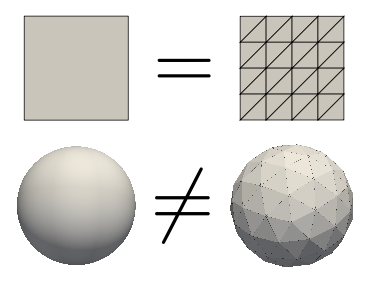
On Euclidean spaces
Just triangulate the domain!
Put the pieces back together, get the original domain!
Main computational tool: FEM
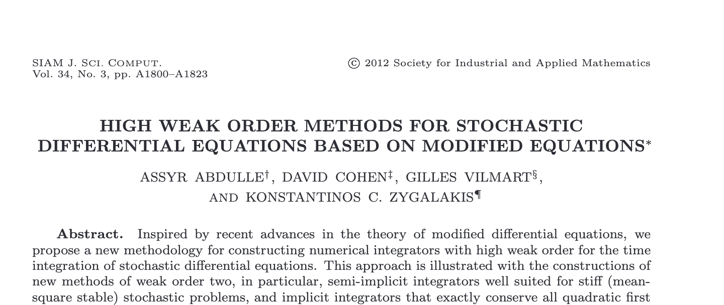
On manifolds!
Step 1: Triangulate the domain
Issue: Approximate solutions live on \(\mathcal{M}_h\), not \(\mathcal{M}\)!
Put the pieces back together, don't get the same domain!
Step 2: FEM space \(S_h \subset H^1(\mathcal{M}_h)\) of p.w., continuous, linear functions
Main computational tool: FEM
On manifolds!
Step 1: Triangulate the domain
Issue: Approximate solutions live on \(\mathcal{M}_h\), not \(\mathcal{M}\)!
Put the pieces back together, don't get the same domain!
Step 2: FEM space \(S_h \subset H^1(\mathcal{M}_h)\) of p.w., continuous, linear functions
Given \(\eta: \mathcal{M}_h \to \mathbb{R}\), \(\eta^\ell= \eta \circ a\) is on \(\mathcal{M}\)!
Step 3: Key tool in surface finite elements: the lift
Takeway: FEM error similar to flat case, up to a "geometry error" term
Main computational tool: FEM
Extra slides: some notes on kernel functions
Euclidean domains
To simulate, specify mean and covariance
- Matérn covariance kernel
- Flexible, used a lot.
- Depends solely on the distance between \(x\) and \(y\).
- Due to stationarity/isotropy.
The sampling question: resolved in isotropic, Euclidean case since the beginning
Euclidean domains
To simulate, specify mean and covariance
- Matérn covariance kernel
- Flexible, used a lot.
- Depends solely on the distance between \(x\) and \(y\).
- Due to stationarity/isotropy.
The sampling question: resolved in isotropic, Euclidean case since the beginning
Curved spaces?
- Idea: replace \(d(x,y)\) with \(d_M(x,y)\) in the Matérn kernel
- Problem: doesn't always work (Gneitling, 2013)
-
Solution: Hand-craft covariance functions?

(Whittle, 1953) Other, more geometric idea: Matérn field on \(\R^d\) solves:
Write down equivalent SPDE on manifold
Curved spaces?
The Laplace–Beltrami operator is a geometric object, so this works for all manifolds
(terms and conditions apply)
Sampling by solving the PDE approximately (numerics has entered!)
Extra slides: paper II
Concrete examples
The operator + model details
The FEM operators
Why not compute e.f.s
Actual matrices used
Details on the
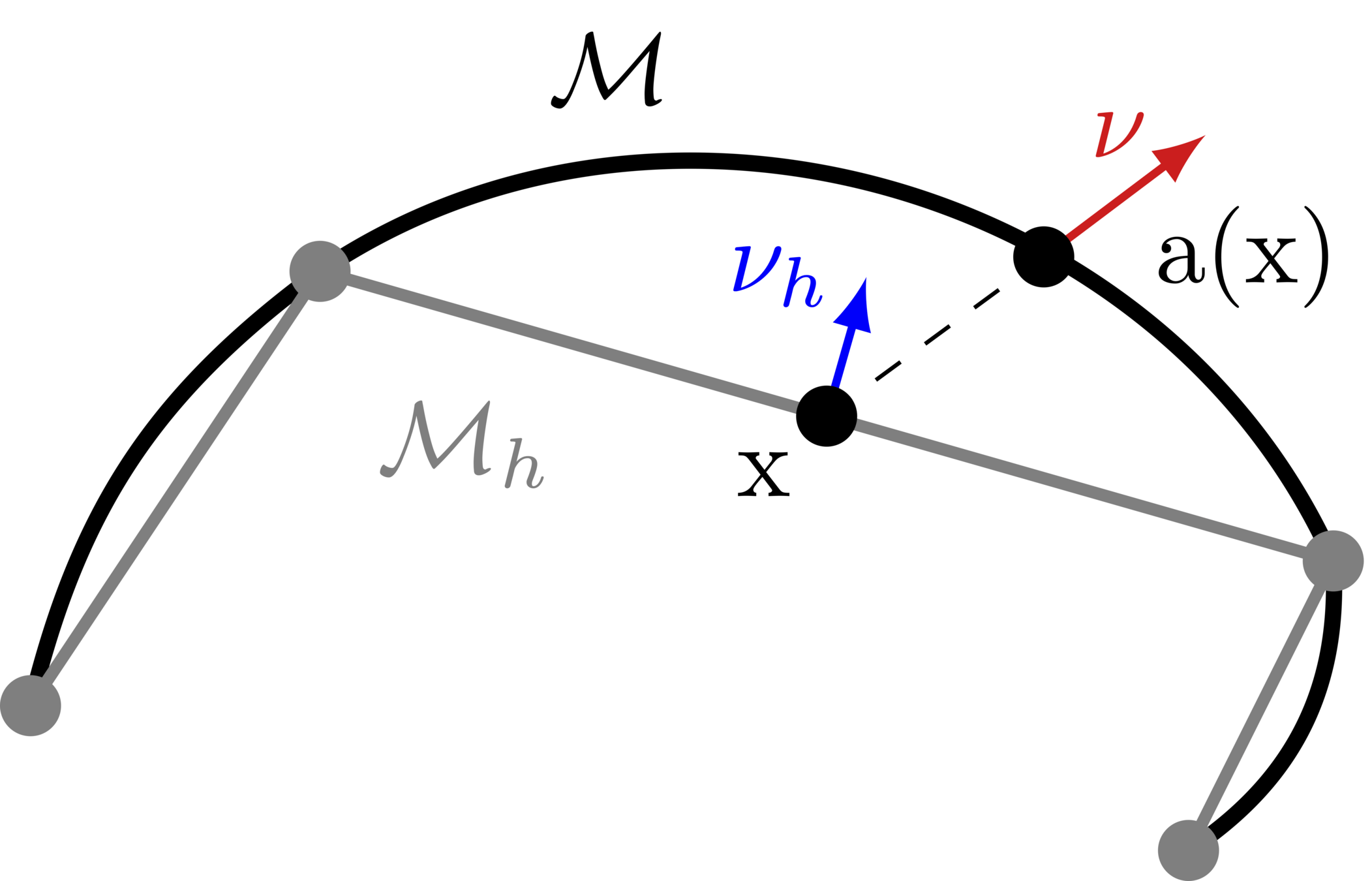
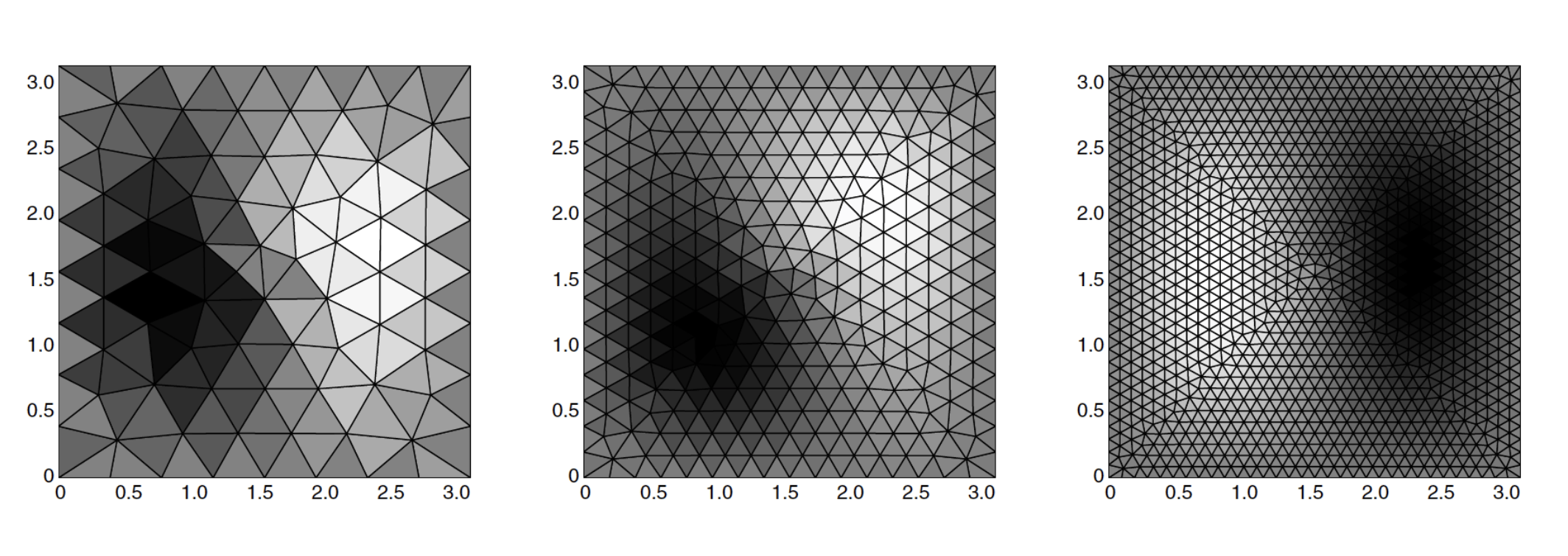
EXTRA: Concrete example I
(Whittle-) Matérn random fields given by SPDE \((\kappa^2-\Delta_{\mathbb{S}^2})^\beta \mathcal Z = \mathcal{W}\)!
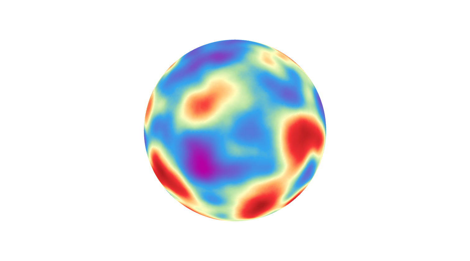
EXTRA: Concrete example II
EXTRA: Concrete example III
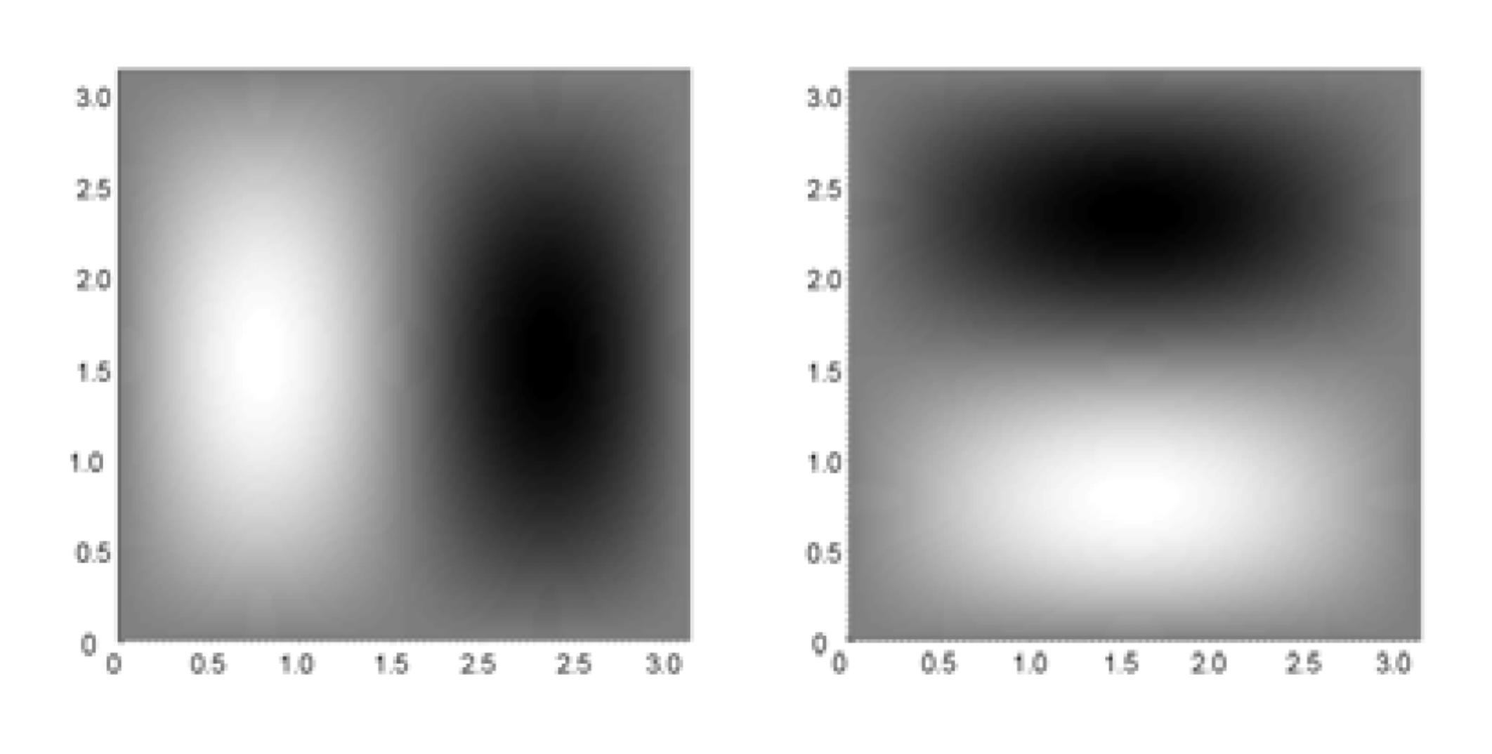
\(\rho_1\) small, \(\rho_2\) large: field is elongated tangentially along level sets of \(f\)
\(\rho_1\) large, \(\rho_2\) small: field is elongated orthogonally along level sets of \(f\)
EXTRA: Concrete example III
EXTRA: More details on the model
Eigenpairs of \( \mathcal{L} \): \((\lambda_i,e_i)\)
+ Conditions
\(\mathsf A_\mathcal{M}\) defines elliptic operator \(\mathcal L\)
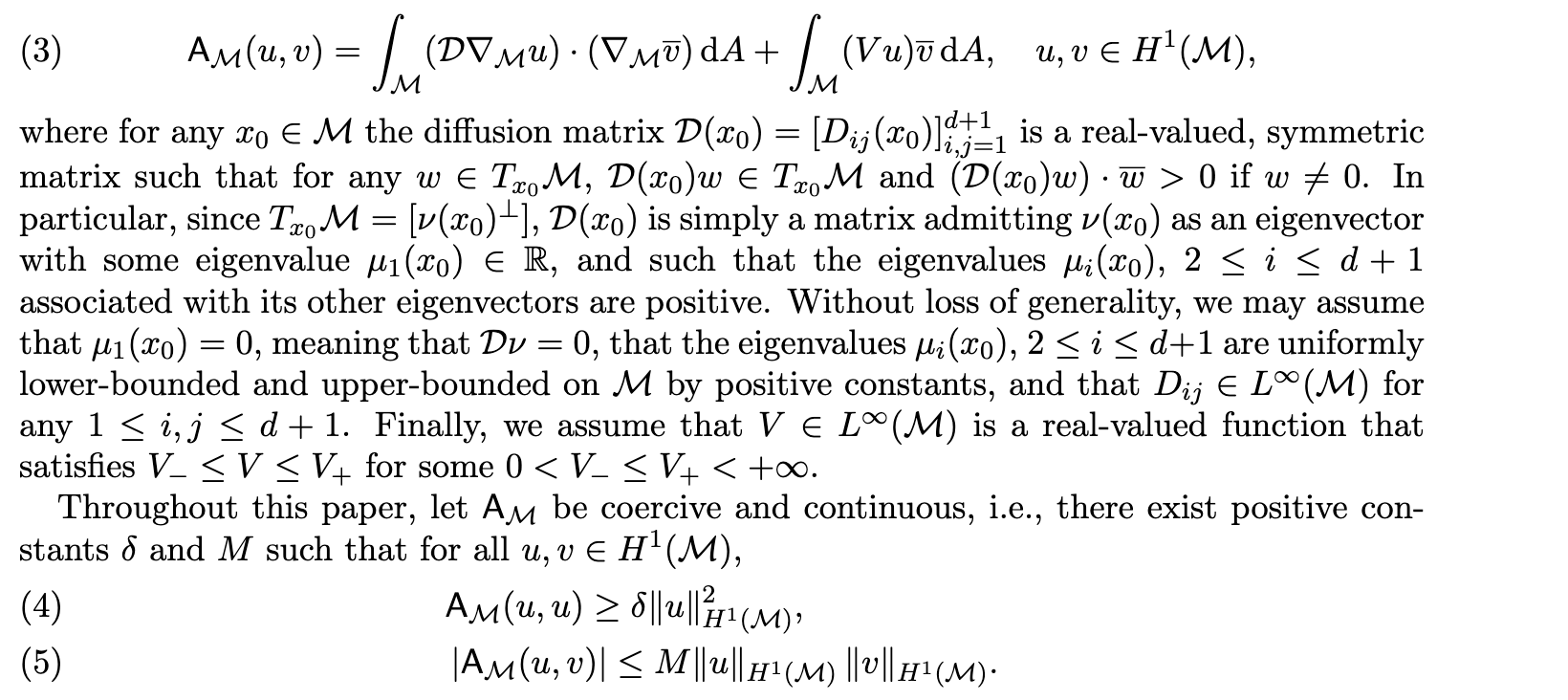
EXTRA: More details on the model
EXTRA: FEM operators
Discretization of operators
Original
Eigenpairs
Discrete 1
Eigenpairs
Discrete 2
Eigenpairs
EXTRA: Why you shouldn't use the EFs
Error analysis:
Problem:
Generally: Approximating eigenfunctions are hard!
Eigenvalues are fine, however!
EXTRA: Why you shouldn't use the EFs
Generally: Approximating eigenfunctions are hard! Multiplicity!
From D. Boffi, Acta Num. (2010)
EXTRA: The matrices involved
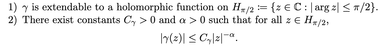
Chebyshev quadrature approximation of \(\gamma\)
Various white noise approximations, various approximations of \(\mathcal Z\)
sd
sd
sd
EXTRA: A small note on the proof...
??
EXTRA: A small note on the proof...
EXTRA: A small note on the proof...
Important result: errors on the form
\(\|\gamma(\mathcal L)f -\gamma(\mathcal L_h) f\|_{L^2}\)
Brief note on proof:
Extra slides: paper III
Geometry of LP systems
Isospectrality
geometric structure of stochastic LP
why not Itô?
proof of convergence, some more details
EXTRA: Geometry of LP systems
Important geometric structure:
LP Systems evolve on coadjoint orbits
(symplectic manifolds that foliate space!)
+ Several preserved quantities, Hamiltonian, Casimirs etc.
Coadjoint orbits
Dynamics on orbit
EXTRA: Geometry of LP systems
\(G \subset \operatorname{GL}(n)\) is compact, simply connected and \(J\)-quadratic, i.e., \(A \in \mathfrak{g} \iff AJ + JA^* = 0 \)
Examples: \(\mathfrak{so}(N), \mathfrak{su}(N), \mathfrak{sp}(N)\).
In this setting, LP flow is isospectral:
EXTRA: Stochastic LP systems
Why Strato?
Why these coefficients?
We need a chain rule
Same bracket-type coefficient: same geometric structure
Stochastic LP Systems evolve on coadjoint orbits and have Casimirs!
EXTRA: Stochastic LP systems
What to assume to prove the existence of solutions?
E.g. Lipschitz is not realistic to assume
But! Some smoothness is sufficient for global existence
System remains on compact level sets of Casimirs
\(\rightarrow\) truncation argument to prove existence
EXTRA: Stochastic LP systems
Stochastic LP Systems evolve on coadjoint orbits and have Casimirs!
Coadjoint orbits
With transport noise
With non-transport noise
EXTRA: Stochastic LP systems
What happens if we apply an off the shelf integrator?
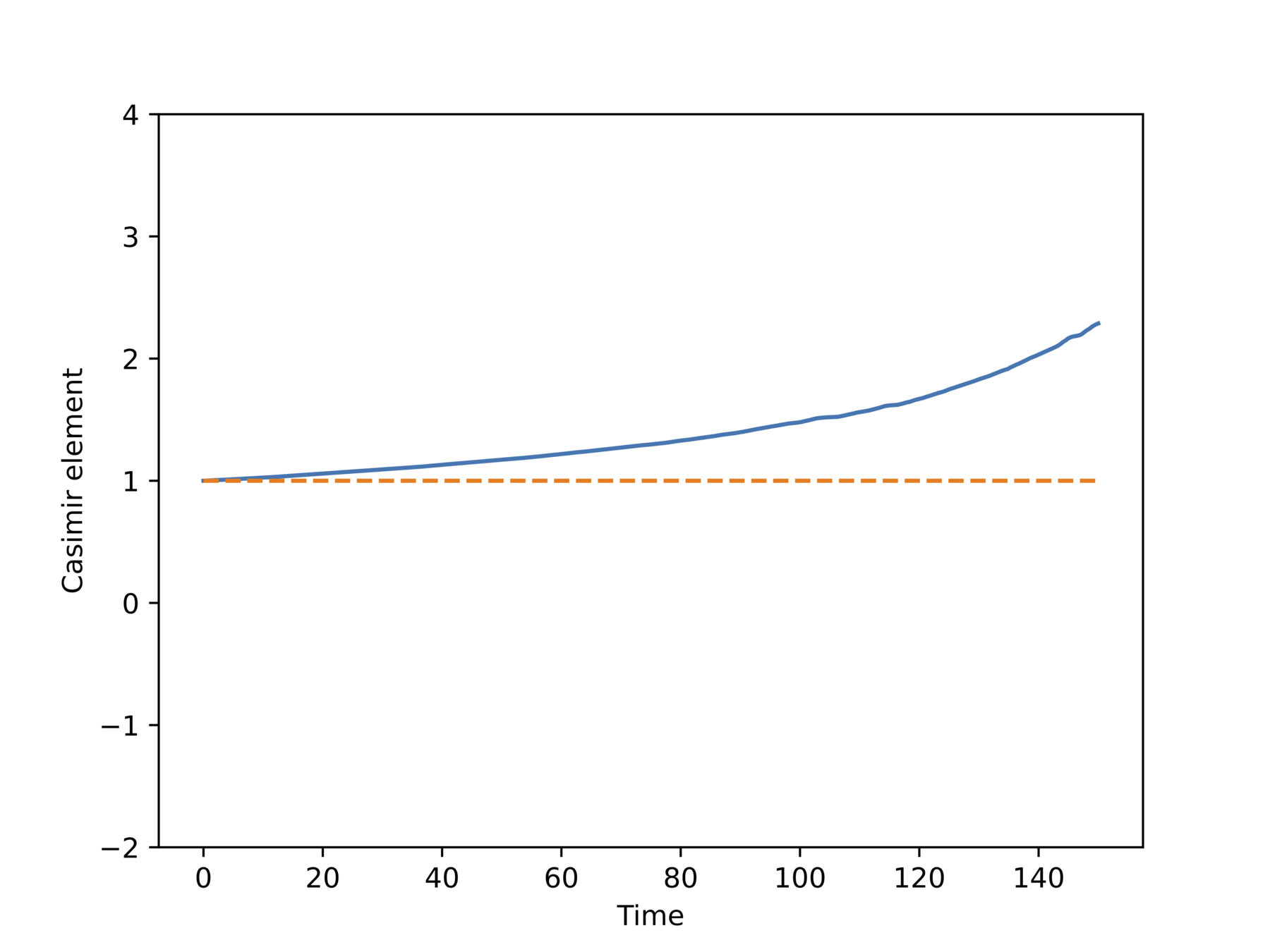
Non-physical behavior!
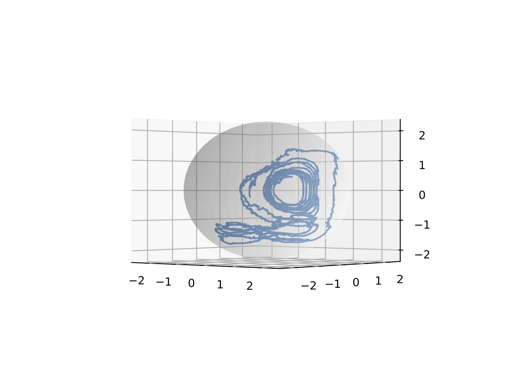
EXTRA: Stochastic LP systems
What happens with structure-preserving integrators?
EXTRA: Unreducing LP systems
Intuitive picture: implicit midpoint in disguise

unresolved unscientific question: if implicit midpoint could wear a disguise, how would it wear it?
Note: No a priori guarantee that this system remains on \(T^*G\)!
Embedded into \((R^{n \times n})^2\) but remains on \(T^*G\)
\(X_t = \mu(Q_t,P_t) \in \mathfrak{g}^*\) satisfies
EXTRA: Integration with tears
EXTRA: Integration with tears
- Symplectic
- Equivariant
- Well-studied
EXTRA: Integration with tears
Stochastic isospectral midpoint:
Take \(Q_n,P_n\) such that \(\mu(Q_n,P_n) = X_n\)
Take \(X_{n+1} = \mu(\Phi_h(Q_n,P_n))\)
Extra: Error analysis with tears
1) Show that the implicit midpoint method does not travel too far:
\(\sup_{h \geq 0} \sup_{n \geq 0} \|Q_n,P_n\| \leq R(Q_0,P_0). \)
2) Truncate the CHS system on \(T^*G\)
Upstairs
Downstairs
3) Apply error analysis from literature
Reduction by \(\mu\)
4) Convergence of method for truncated LP system
- Strong convergence: \(\mu\) is Lipschitz
- Weak convergence: \(\phi \circ \mu\) is valid test func
5) Truncated LP system = LP system
Recipe:
Extra: Error analysis with tears
- Assume: \(H_0 \in C^4\) and \(H_1,H_2, \ldots, H_M \in C^5\).
- \(T>0\): be a fixed final time,
- \(N \in \mathbb{N}\): number of steps
- \(X_0 \in \mathfrak{g}^*\): Deterministic initial condition
- \(\phi \in C^5\): Test function
Extra: Error analysis with tears
- Assume: \(H_0 \in C^4\) and \(H_1,H_2, \ldots, H_M \in C^5\).
- \(T>0\): be a fixed final time,
- \(N \in \mathbb{N}\): number of steps
- \(X_0 \in \mathfrak{g}^*\): Deterministic initial condition
- \(\phi \in C^5\): Test function
Extra: Error analysis with tears
Geometric structure of equations and its preservation is central. Used to prove
- Existence and uniquness
- Convergence
Without structure preservation, no convergence guarantees
Extra slides: IsoMP vs other methods
- Explicit methods based on splitting for separable Hamiltonians
- Extend to \(T\operatorname{GL}(n)\), use symplectic RATTLE
- Symplectic Lie group methods on \(T^* G\), map back and forth with exponential map
- Collective symplectic integrators
- IsoMP works directly on algebra
- no constraints
- no algebra-to-group mappings
- works for large class of Hamiltonians
Extra slides: generalities on shape matching
How to match?
Idea: Use a distance \(d_V\colon V \times V \to \mathbb R\) on \(V\), look for \(g \in G\) that solves
How to match \(A \in V \) with \(B \in V\)?
Problem: In general, no \(g\) takes \(A\) to \(B\) \(\implies\)
more and more complex warps of \(A\)
(the action is non-transitive).
Regularize!
Regularize!
Add a regularization term!
Penalize strange deformations
How to compute \(d_G(e,g)\)?
Pricey! An optimization problem in itself!
The simpler way: Let \(d_G\) be the distance function of a right-invariant Riemannian metric and generate \(g\) as a curve! (Geometry!)
Let it flow
Let it flow
\({\color{#a64d79}{\nu}}\colon [0,1] \to \mathfrak{g}\) is a curve in the vector space \(\mathfrak{g}\)!
Let right-invariance strike!
Let it flow
An optimization problem over curves in a vector space!
\({\color{#a64d79}{\nu}}\colon [0,1] \to \mathfrak{g}\) is a curve in the vector space \(\mathfrak{g}\)!
Let right-invariance strike!
Extra: Ingredients for shape analysis
- A Lie group of deformations \(G\) acting on a set of shapes \(V\) (metric space)
- A fidelity energy that evaluates the closeness of two shapes
- A regularization energy that penalizes aggresive deformations
Flexible choice
Right-invariant metric (not so flexible)
Extra slides: paper IV
Extra: Paper IV
In usual LM, all vector fields are available
Idea: Constrain set of vector fields
Sub-Riemannian landmark matching!
Landmark matching:
\(V = (\mathbb{T}^2)^N\),
\(G = \operatorname{Diff}(\mathbb{T}^2)\)
Extra: Paper IV
\(\mathcal{S}\)
\(v = F(u)(x)\)
\(\mathfrak{X}(M)\)
\(F(u)\)
\(\mathcal{U}\)

\(u\)
Extra: Paper IV
\(\mathcal{S}\)
\(v = F(u)(x)\)
\(\mathfrak{X}(M)\)
\(F(u)\)
\(\mathcal{U}\)
\(u\)
Extra: Paper IV
Dynamics of \(u\) are determined from the dynamics of \(v\)
Instead of optimizing over vector fields, optimize over \(\mathcal{U}\)
\(\mathcal{U}\) is finite dimensional \(\implies\) discretization
How to find dynamics of \(u\)?
Idea: Apply chain rule to \(\dot m = \operatorname{ad}_v^T m\)
Extra: Paper IV
\(\mathcal{S}\)
\(v = F(u)(x)\)
\(\mathfrak{X}(M)\)
\(F(u)\)
\(\mathcal{U}\)
\(u\)
Extra: Paper IV
Connected to neural networks!
Infinite number of layers \(\implies\)
Time-continuous optimal control problem
Skip connection \(\implies \) Explicit Euler
Extra: Paper IV
When matching landmarks, points are moved by a vector field parametrized by some control variable.
A neural networks moves points along a vector field determined by weights and biases.
Extra: Paper IV
- Landmarks
- Image
- Warping new landmarks
- Control parameters
- Input data, e.g. images
- "Meta-image"
- Testing
- Weights and biases
View networks with shape analysis glasses!
Extra slides: paper V
Extra: Paper V


Extra: Paper V
Geometric structure


In brief: Gradient flow horizontally or vertically
(More info: Modin, 2017 and references therein)
Gaussian Monge Problem:
\(\mu_0\) and \(\mu_1\) are both (zero-mean) normal distributions on \(\mathbb{R}^n\).
Normal distributions \(\cong\) \(P(n)\), positive-definite symmetric matrices


Extra: Paper V
Extra: Paper V
In brief: Gradient flow horizontally or vertically
Extra: Paper V
How to prove convergence?
Idea: Show \(\frac{\mathrm d} {\mathrm d t} J \to 0\), and that this means we hit polar cone
Extra slides: paper VI
Shooting,
Gradient
Quantitative results
The dynamic formulation
Matching by shooting
Recall example II from intro: reduction to dynamic formulation is made easy by right-invariance
Shape for Cryo-EM
Gradient is available
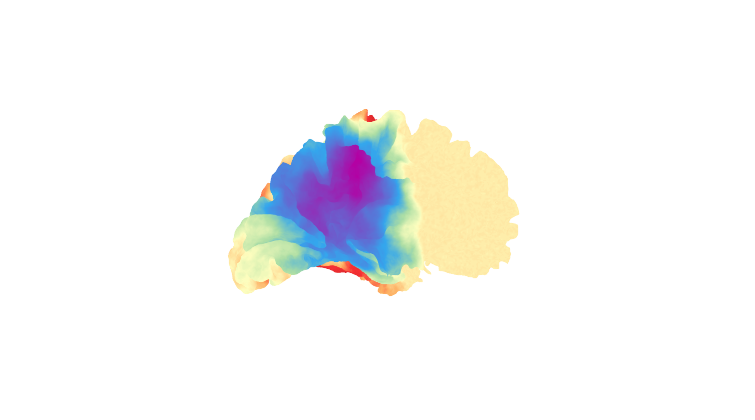
Extra: three deformations
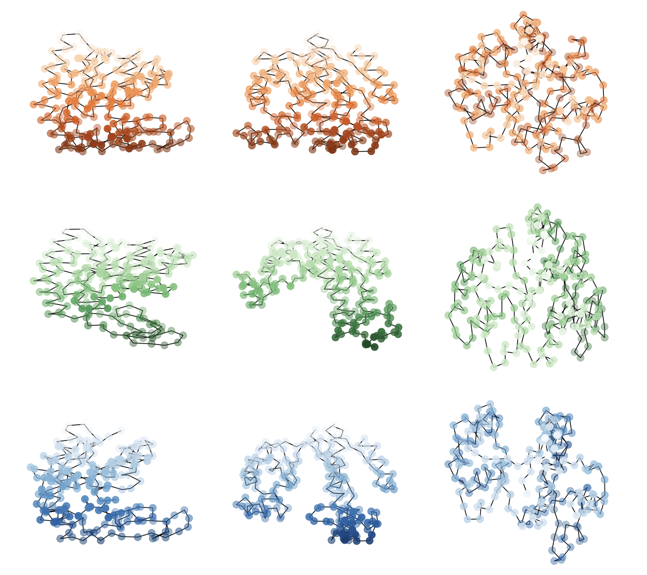
x
y
z
Deformed
Target
Template
Extra: quantitative
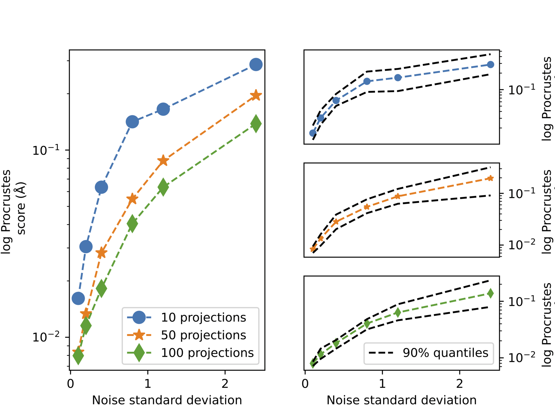
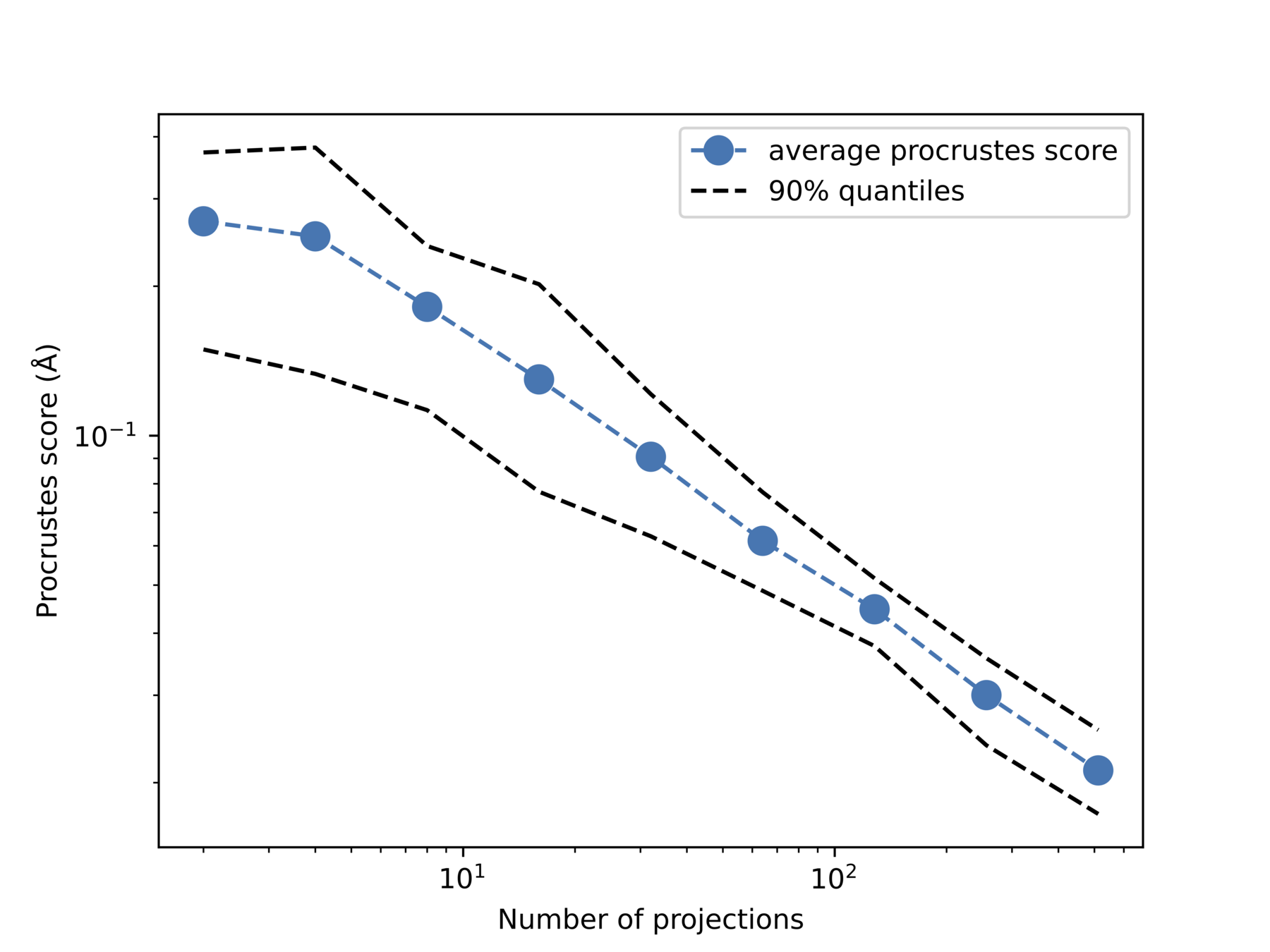
Increase noise
Increase #projections
Quantative measure: Procrustes score
Extra slides: paper VII
Euler equations
Zeitlin
Complexified Euler equations
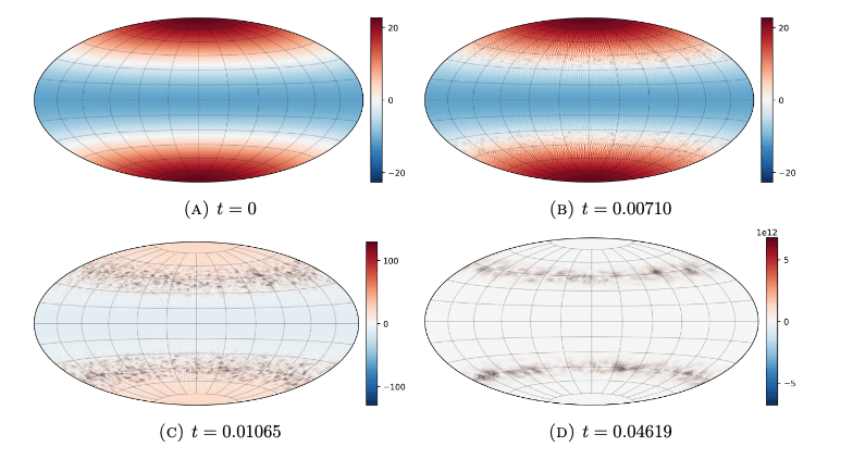
Simulations for Blow-up
Extra: Paper VII
The \(L^2\)-geodesic equation on \(\operatorname{Diff}_{\mu}(\mathbb{S}^2)\):

Extra: Paper VII
Euler eqs: Lie-Poisson system on \(C^\infty_0(\mathbb{S}^2) \cong (\mathfrak{X}_\mu(\mathbb{S}^2))^*\)

=> Sphere is Kähler
Initially for the torus, but we work on the sphere!
Extra: Paper VII
Goal: Find a mapping \(T_N:C_0^\infty(\mathbb{S^2}) \to \mathfrak{su}(N)\) such that:
Hoppe, 1989:
How to find \(T_{l,m}^N\)?
Extra: Paper VII
Coordinate function representation of \(\mathfrak{so}(3)\) in \((C^\infty_0(\mathbb{S}^2),\{\cdot,\cdot\})\).
Spin \(s = (N-1)/2\)-representation of \(\mathfrak{so}(3)\) in \(\mathfrak{u}(N)\)
Extra: Paper VII
Hoppe–Yau Laplacian:
Hoppe–Yau (1998):
The first \(N^2\) eigenvalues of \(\Delta\) coincides with those of \(\Delta_N\)
\(T_{l,m}^N\) are eigenfunctions to \(\Delta_N\)
Extra: Paper VII


Extra: Paper VII
Quantized system on \(\mathfrak{su}(N)\):
Continuous system on \(C^\infty_0(\mathbb{S}^2)\):
Extra: Paper VII
Canonical expression (EP-equations):
Relationship between \(\omega\) and \(\psi \)?
Consider complexified Euler equations as LP system on complexified functions:
Extra: Paper VII
Relationship between \(\omega\) and \(\psi \)?
Determined by Hamiltonian!
Math
Proven to blow up in finite time for toroidal case. Conjecture same is true for numerics
Extra: Paper VII
How to detect in numerics?
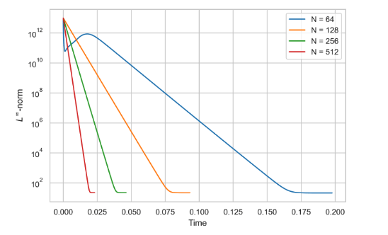
Grows very rapidly
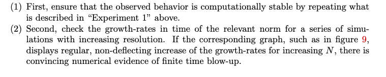
How to be sure that the observed behavior is not a numerical artifact?
Extra: Paper VII
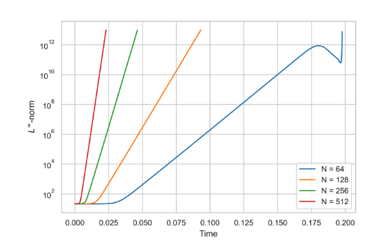
Growth of norm!
Extra: Paper VII
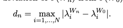
Check spectral deviation
Extra: Paper VII
Check reversibility
Extra: Paper VII
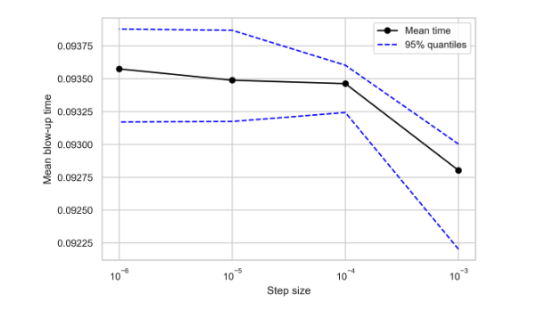
Check mean time to blow up wrt step size -stabilizes
Extra: Paper VII
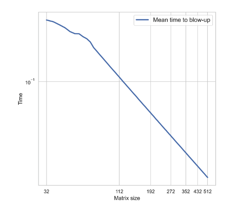
Check mean time to blow up wrt matrix size
Extra: Paper VII: signature
Linear growth after transient phase?
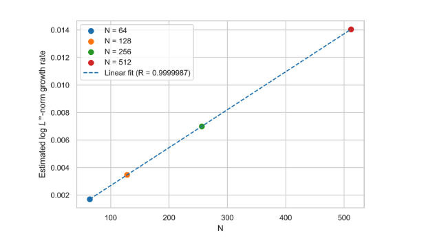
Linear rate vs matrix size - linear relationship
Extra: Paper VII: signature
Extra slides: notes on Zeitlin
Why not the torus?
Generator of isometries:
Generator of isometries:
