How to compute the polar factorization of a matrix in a way you shouldn't
The Monge problem


Geometric structure


In brief: Gradient flow horizontally or vertically
(More info: Modin, 2017 and references therein)
The Gaussian Monge problem
\(\mu_0\) and \(\mu_1\) are both (zero-mean) normal distributions on \(\mathbb{R}^n\).
Normal distributions \(\cong\) \(P(n)\), positive-definite symmetric matrices


Geometric structure
Geometric structure
In brief: Gradient flow horizontally or vertically
Vertical matrix flow
E.J, K. Modin, Convergence of the vertical gradient flow for the Gaussian Monge problem J. Comput. Dyn. (accepted), 2023
How to prove convergence?
Idea: Show \(\frac{\mathrm d} {\mathrm d t} J \to 0\), and that this means we hit polar cone
Questions!
Convergence rate in linear case?
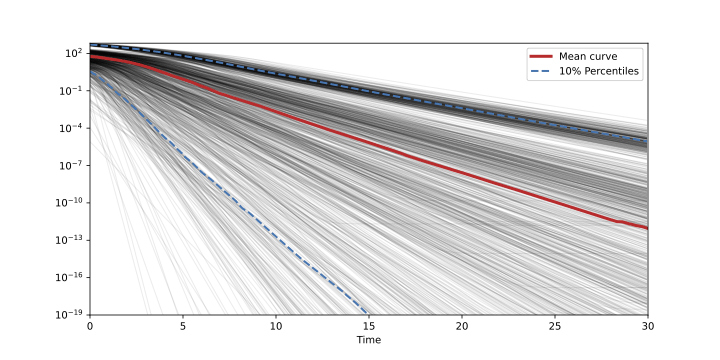
Random matrices with known factorization \(A = PU\), distance to \(B\) from \(P\).
Interesting for other, similar matrix flows.
Questions!
Gaussian case: pre-study for more work into the gradient flows in the infinite-dimensional case?
- Existence? Convergence to minimizer?
- Discretization?
Polar decompositions
Decompose a matrix into one orthogonal part and one symmetric p.d. part
Polar decompositions
Decompose a matrix into one orthogonal part and one symmetric p.d. part
Polar decompositions
Easy to do in for instance python
import numpy as np
from scipy.linalg import polar
a = np.array([[1, -1], [2, 4]])
u, p = polar(a, 'left')
Algorithm is based on SVD factorization, ~0.01 ms (including overhead)
Polar decompositions the hard way
Matrix ordinary differential equation!
- Plug into favorite matrix ODE solving algorithm that preserves structure (expensive)
- Run flow "until convergence"
In the end: \(B(\infty) = ????\)
To compute the polar decomposition of a matrix \(A\):
Take a known and fixed symmetric and positive definite matrix \(\Sigma_0\) and solve the following matrix ODE until \(t = \infty\):
The algorithm: implemented
import numpy as np
from scipy.linalg import solve_sylvester,expm, polar
A = np.array([[1, 1], [2, 4]])
Sigma0 = np.eye(2)
Sigma1 = A@Sigma0@A.T
T,h = 60,0.1 #Integration params: final time, step size
B = A
for _ in range(int(T/h)):
    Omega = solve_sylvester(Sigma1,Sigma1,2*Sigma1@(np.linalg.inv(B)-np.linalg.inv(B).T))
    B = expm(h*Omega)@B
Much more complicated! solve_sylvester hides stuff, expm is expensive. Total time: ~ 300 ms
The algorithm: i n a c t i o n
- Slow! When size grows, algo slows :(
- When has it converged enough?
- Much superior and optimized algos available
Why is it still interesting?
- So, the algo is crap
- But still, the thesis work I found the nicest and most rewarding
Interest lies in how the method arises.
Questions I think I should have raised:
- How did you come up with that?
- Why does it converge to the symmetric factor like that?
OPTIMAL TRANSPORT
The answer:


Optimal transport
The Gaussian Monge Problem
\(\mu_0\) and \(\mu_1\) are both (zero-mean) normal distributions on \(\mathbb{R}^n\): Parametrized by choice of p.d. symmetric covariance matrix
The statistical manifold of normal distributions is the set \(P(n)\) of positive-definite symmetric matrices
(REFERENCE: INFORMATION GEOMETRY, AMARI)
The Gaussian Monge Problem
The geometry of the GaussMP
Geometry? You work with manifolds and stuff... \(\operatorname{GL}(n)\) is a manifold.
Manifolds have tangent spaces
(they contain tangent vectors!)
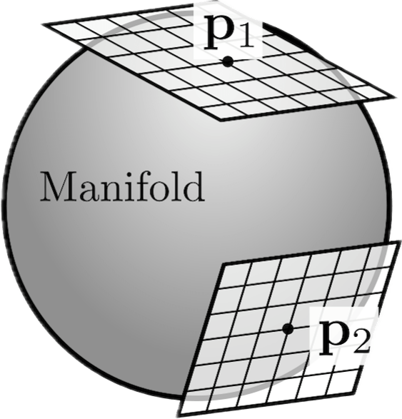
Manifolds can be equipped with Riemannian metrics (generalizations of Euclidean i.p.) that are inner products on each tangent space
The geometry of the GaussMP
Let's put a metric on \(\operatorname{GL}(n)\)
The metric induces a distance function on \(\operatorname{GL}(n)\)
By a fantastic coincidence, \(J(A) = d^2(I,A)\)
The solution to the GaussMP is known!
The geometry of the GaussMP
By Breniér's theorem, the solution of the GaussMP is the positive-definite symmetric part of the polar decomposition!
The geometry of the GaussMP
- \(\operatorname{GL}(n)\) is a Lie group
- It acts on \(P(n)\) by \(A.\Sigma = A \Sigma A^T\)
- This action is transitive, i.e., any two matrices in \(P(n)\) can be connected by one in \(\operatorname{GL}(n)\)
- The action thus defines a projection \(\pi(A) = A \Sigma_0 A^T \in P(n) \)
- The Lie subgroup \(\operatorname{O}(n,\Sigma_0)\) are the matrices that leave \(\Sigma_0\) unchanged, i.e., \(\pi(Q) = \Sigma_0\)
- Finally: \(\operatorname{O}(n,\Sigma_0)\) is isomorphic to \(C(\Sigma_0,\Sigma_1)\)
This is what in the business is known as a principal \(\operatorname{O}(n,\Sigma_0)\)-bundle, with fibers \(\pi^{-1}(\Sigma) \)
The geometry of the GaussMP
The geometry of the GaussMP
The Fiber above the \(\Sigma_0\) is \(\operatorname{O}(\Sigma_0,n)\)
The tangent spaces of \(\operatorname{GL}(n)\) splits into vertical component along fiber and horizontal perpendicular to fiber
The polar cone is all the horizontal geodesics connected to the identity. The polar cone is isomorphic to \(P(n)\)
Theorem: there is a unique element of the polar cone in \(\pi^{-1}(\Sigma_1)\) This is the solution to the OT problem.
Finding the matrix ODE
Use gradient flows to minimze \(J(A)\)! Restrict metric to \(\pi^{-1}(\Sigma_1)\), and compute
\(\dot B = -\nabla_{\mathcal G|_{\pi^{-1}(\Sigma_1)}} J(B), B(0) = A \)
Other GFs are available, along the polar cone, directly in the covariance matrices, etc.
Finding the matrix ODE
How to prove that this converges to \(P\)?
- Prove that the flow exists for all time
- Prove that as \(t \to \infty\), \(\frac{\mathrm d }{\mathrm d t} J(B) \to 0\),
- Prove that this in turn is equivalent to \(B(\infty) \in K_\diamond\)
- Use that the intersection of fiber and \(K_\diamond\) only contains one element!
Just a theoretical exercise?
The geometric structure is the same in the general OT case. Corresponding flow can be derived!
- Existence? Convergence to minimizer?
- Discretization?