Gradient flows for
indirect matching
problems
Erik Jansson

Joint work with:

Klas Modin (Chalmers Uni)
Carola-Bibiane Schönlieb
(Cambridge)
Ozan Öktem (KTH)
Jonathan Krook (KTH)


in 30 seconds (by a maths person)
Electron
microscope

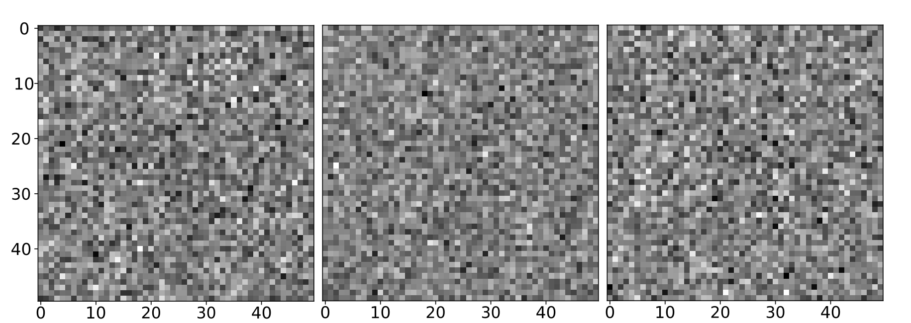
Low dose: low SNR
Many images
Many copies of the same protein but at different orientations and conformations
Particle picking
Reconstructing from Cryo-EM data
Reconstructing from Cryo-EM data
Issue: SNR is around 0.01-0.001, so almost no information
Could the problem be made easier if we knew which protein
was imaged and that we are observing a deformation of a representative conformation?
Hint: Yes, this incorporates an
"anatomical prior"
Reconstructing from Cryo-EM data
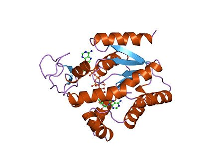
Goal to reconstruct
Template
Reconstructing from Cryo-EM data
3D reconstruction results
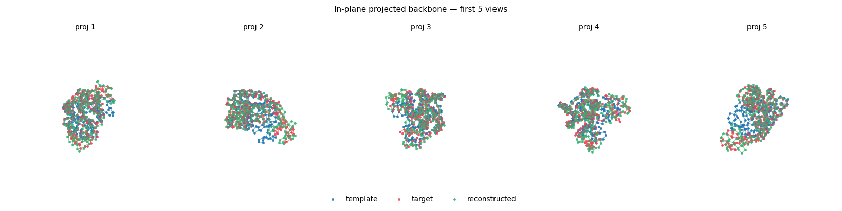
2D projection results
Tomography
in 30 seconds (by a maths person)
X-ray tube
Test object
Detector
Rotation
Tomography
We consider the limited angle (angle X-ray tube can slide to most 60 degrees)
sparse (only six angles) tomography.
Data
Target
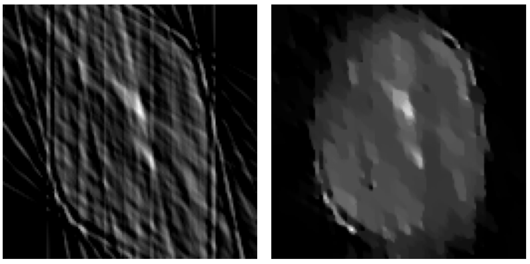
Two classic reconstructions
"Our" reconstruction
Same principle
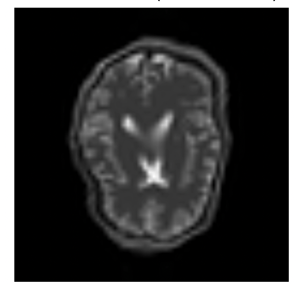
We are imaging a brain: anatomical prior
Data
Target
Template
Same principle
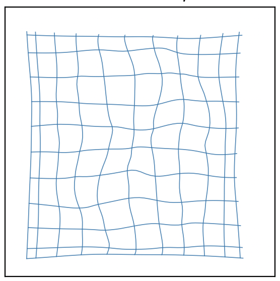
Deform a template to match an indirectly observed target
Stage is set for some shape matching!
Shapes are in a (metric) space \(V\) acted upon by a Lie group of deformations \(G\).
Quick background (LDDMM)
Deformations \(\gamma\) is endpoint of curve \(\gamma \colon [0,1] \to G \)
Right-invariance of metric
Indirect matching (LDDMM)
Geometric framework remains the same.
- Group \(G\) acting on shape space \(V\)
- Data is in data space \(Y\) (Hilbert)
Include a forward operator \(\mathcal{F}\colon V \to Y\)
Reconstructs the \(\gamma(1).A\) that best would map to \(B\)
Indirect matching (LDDMM)
- LDDMM framework remains the same, solve by shooting or your favourite algorithm
- However, framework remains slow (additional variables introduced)
- Gradient contains adjoint of differential of forward map: nonlinear FM => optimization issues
- Experience tell us LDDMM-based reconstruction works very well, though (at least for the two examples seen earlier)
Following Balehoskwy, Karlsson and Modin, there might be a faster way
Gradient flow directly on the group
Indirect matching (LDDMM)
Gradient flow directly on the group
Gradients are Riemannian object, so equip \(G\) with a right-invariant metric.
Translate vectors back to algebra, map one to dual with inertia operator, take duality pairing
Gradient computation via momentum map
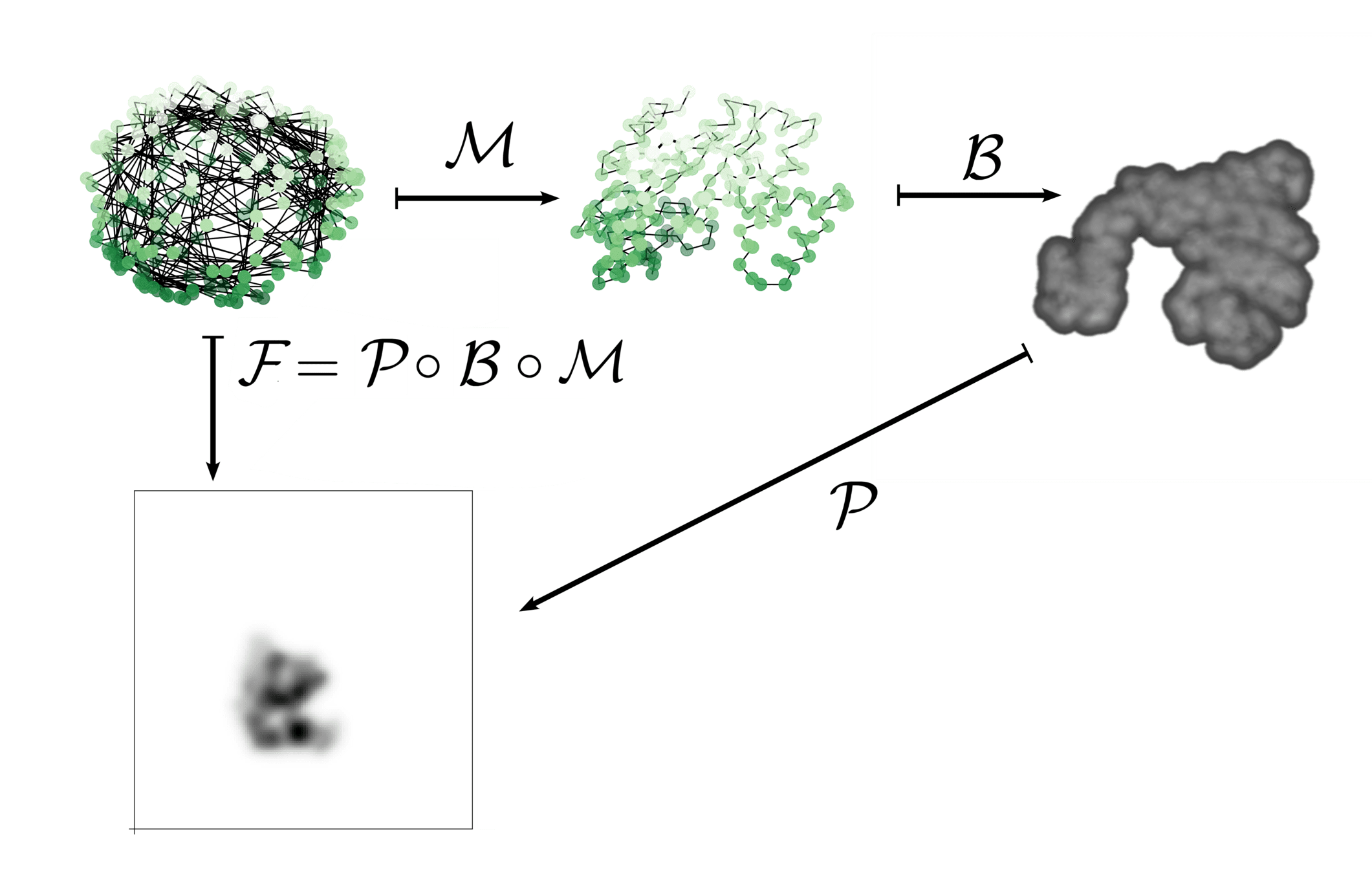
The Lie group action on the shape space induces a momentum map
Let \(f\colon V \to \R\) and take \(E(g) = f(\Phi(g,w))\)
\(\Phi\colon G \times V \to V\) is the group action
Let \(y \in Y\) be observed data
Set \(f = \mathcal{L}_y \circ \mathcal{F} \) for data loss function \(\mathcal{L}_y \colon Y \to \mathbb{R} \) and forward model \(\mathcal{F}\colon V \to Y\)
Then \(E(g) = \mathcal{L} \circ \mathcal{F} \circ \Phi(g,w)\) is a indirect matching loss!
Gradient flows!
We would like to minimize:
So we run:
A question: isn't this just greedy matching?
No, because we can easily regularize: Extend shape space \(V' = V \times V_R\), where the action of \(G\) on \(V_R\) is something that we should keep small (i.e., metric, background density, etc. Depends on group and problem)
Back to where we started, proteins
Goal to reconstruct
Template
Protein modelling
Proteins in 30 seconds (by a mathematician)
In this work: forget about everything but the \(C_\alpha\)s
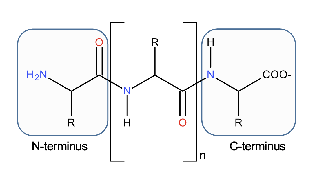
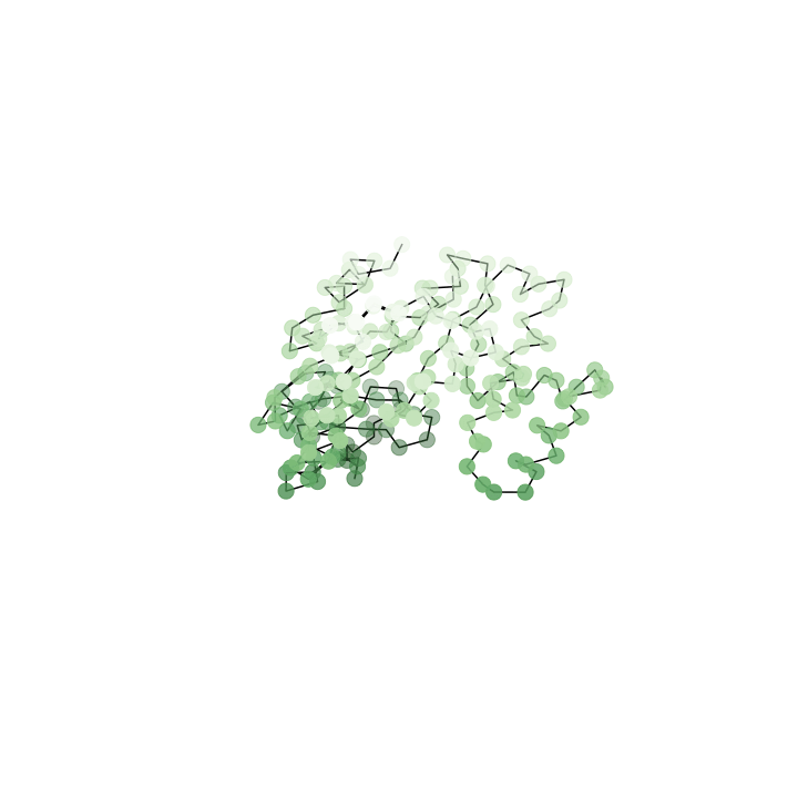
Relative positions
\((\mathbb R^3)^N\)
Mathematical model for proteins
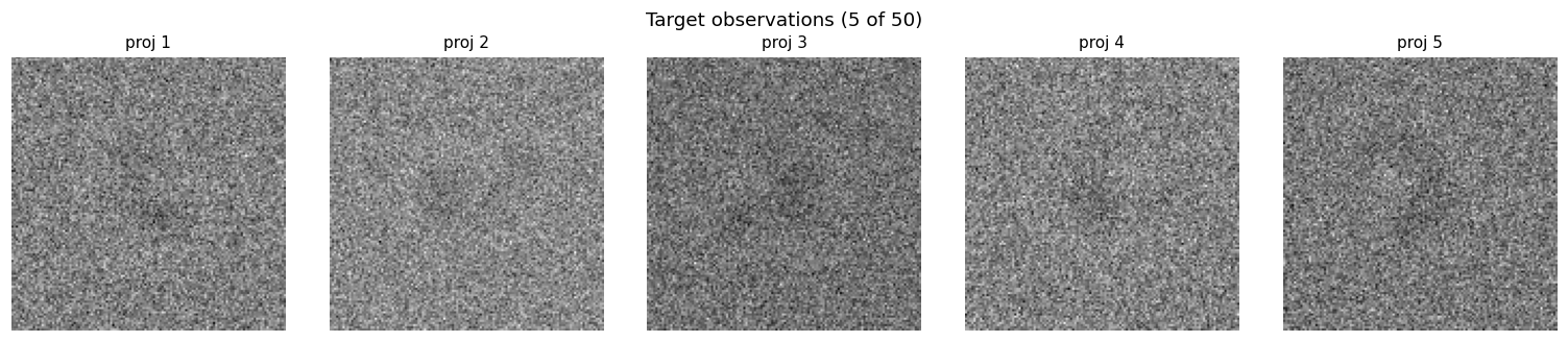
Set-up and forward model
Shape space: space of relative positions \(V = \mathbb{R}^{3N}\)
Data space - M 2D images, \(L^2(\mathbb{R}^2)^M\)
We want rigid deformations, so \(G = \operatorname{SO}(3)^N\)
Action of rotations on relative positions ensures that a deformed protein backbone looks like a protein backbone
Forward model and data fidelity
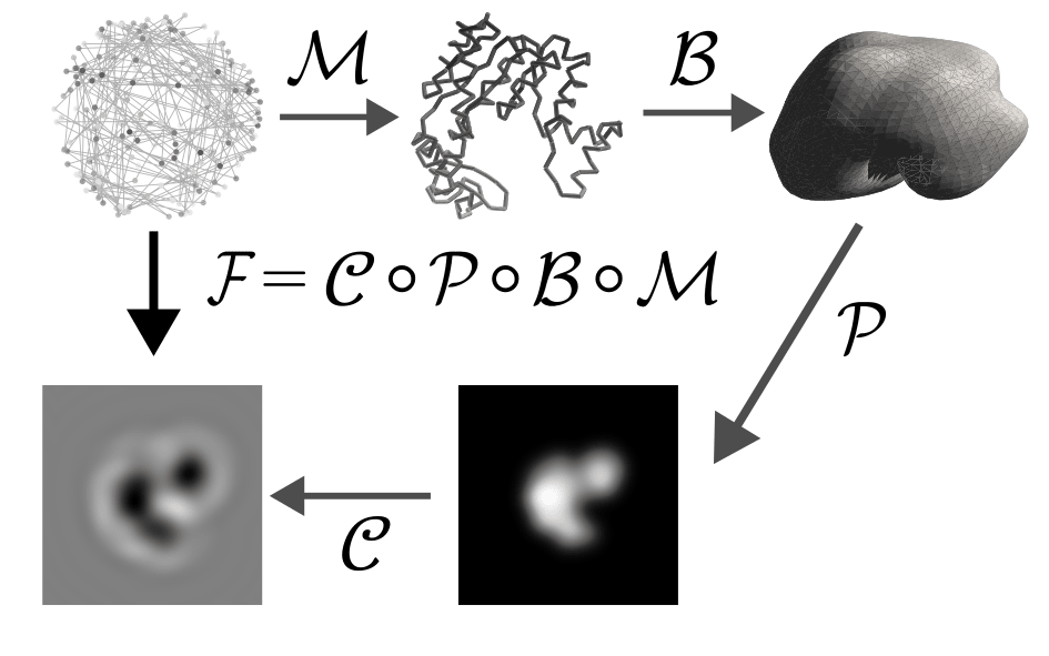
In the end: Each image with one projection and forward model \(\mathcal{F}_j, j = 1,\ldots, M\)
We use NCC as a similarity measure, i.e., \(\mathcal{L}_y(y') = \sum_i \alpha_i(1-\frac{\langle y_i,y_i'\rangle}{\|y_i\|\|y_i'\|})\)
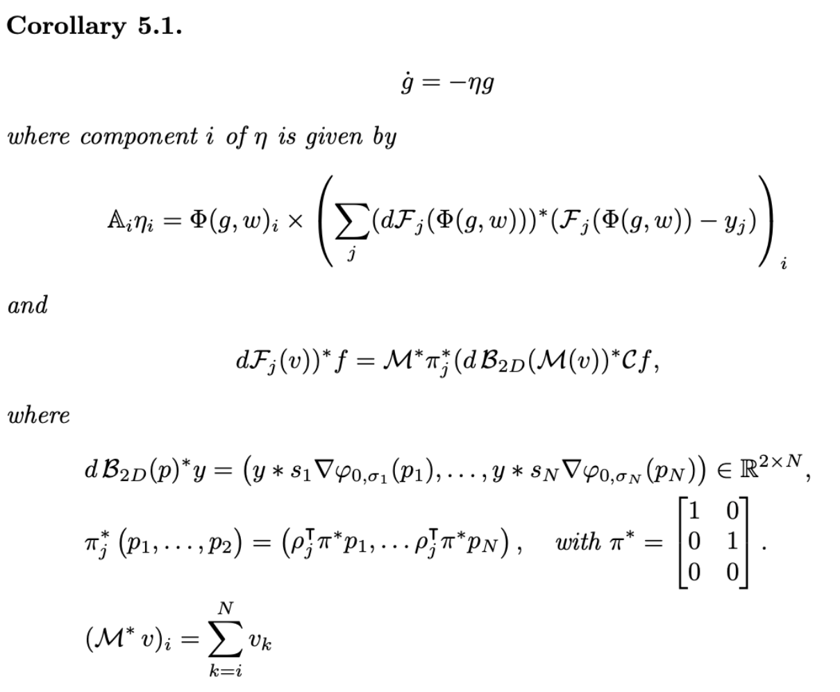
Protein gradient flow derivation
Group action \(\Phi\) by element-wise multiplication,
momentum map is angular momentum in each component
\(y_1, \ldots y_M\) are micrographs,
The adjoint is easy to derive but results in rather unaesthetic expression
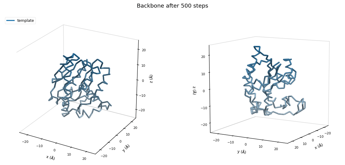
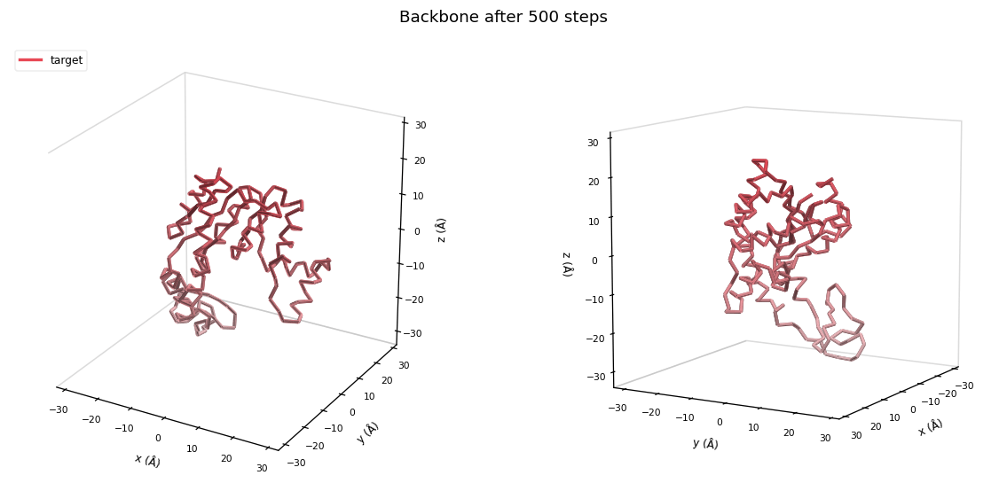
Gradient flow
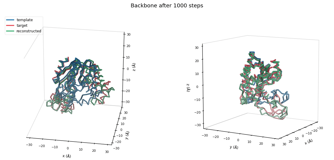
3D reconstruction results
210 residues, ADK, one chain (monomer)
3D reconstruction results
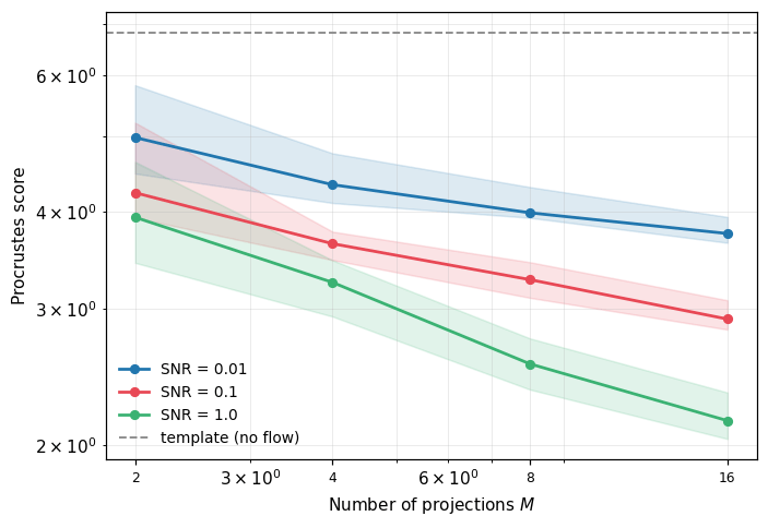
More projections = Good
Less noise = good
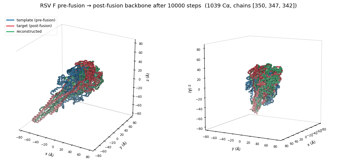
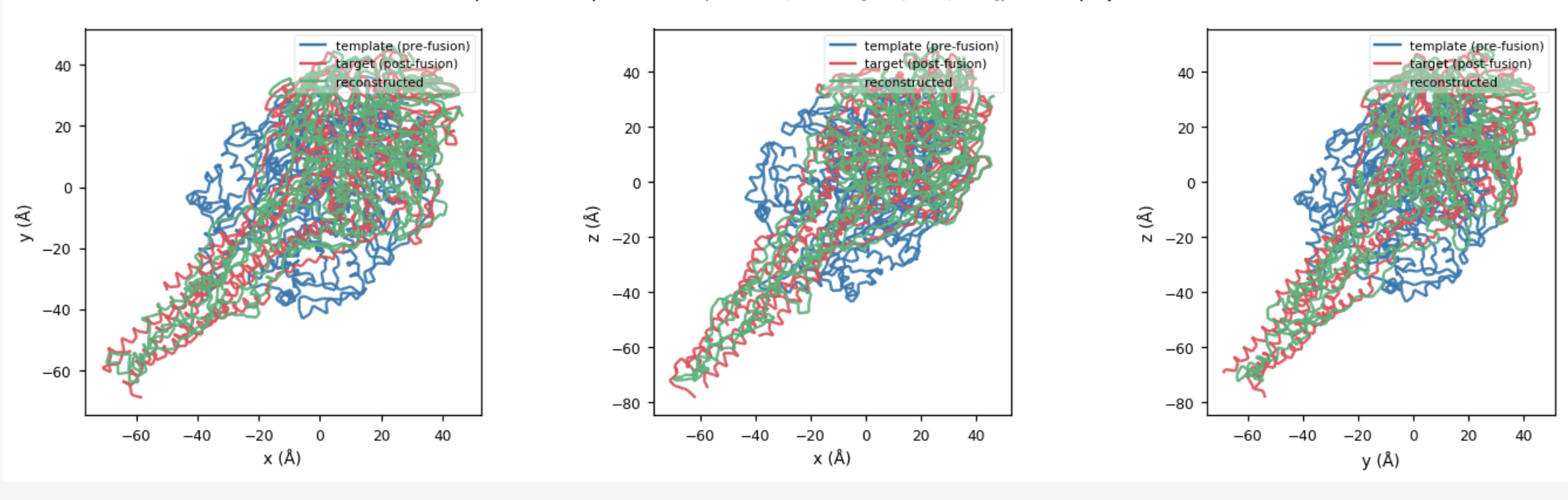
3D reconstruction results
Reconstruction to multimer proteins is straightforward.
Here: 3 Chains, each of ~340 residues, in total 1039 residues
Note on well-posedness
In finite dimensions
(on a compact group)....
Global well-posedness is easy to prove!
As are the properties of the IP
Tomography setup
- Classical set-up: \(G = \operatorname{Diff}(M), V = C^\infty(M), Y =L^2(S^1\times \mathbb{R}) \)
- Forward operator \(\mathcal{F}\colon \to L^2(S^1 \times \mathbb{R})\) is the ray transform.
For one beam parametrized by \((\theta \in S^1, t \in \mathbb{R})\), its value is given by
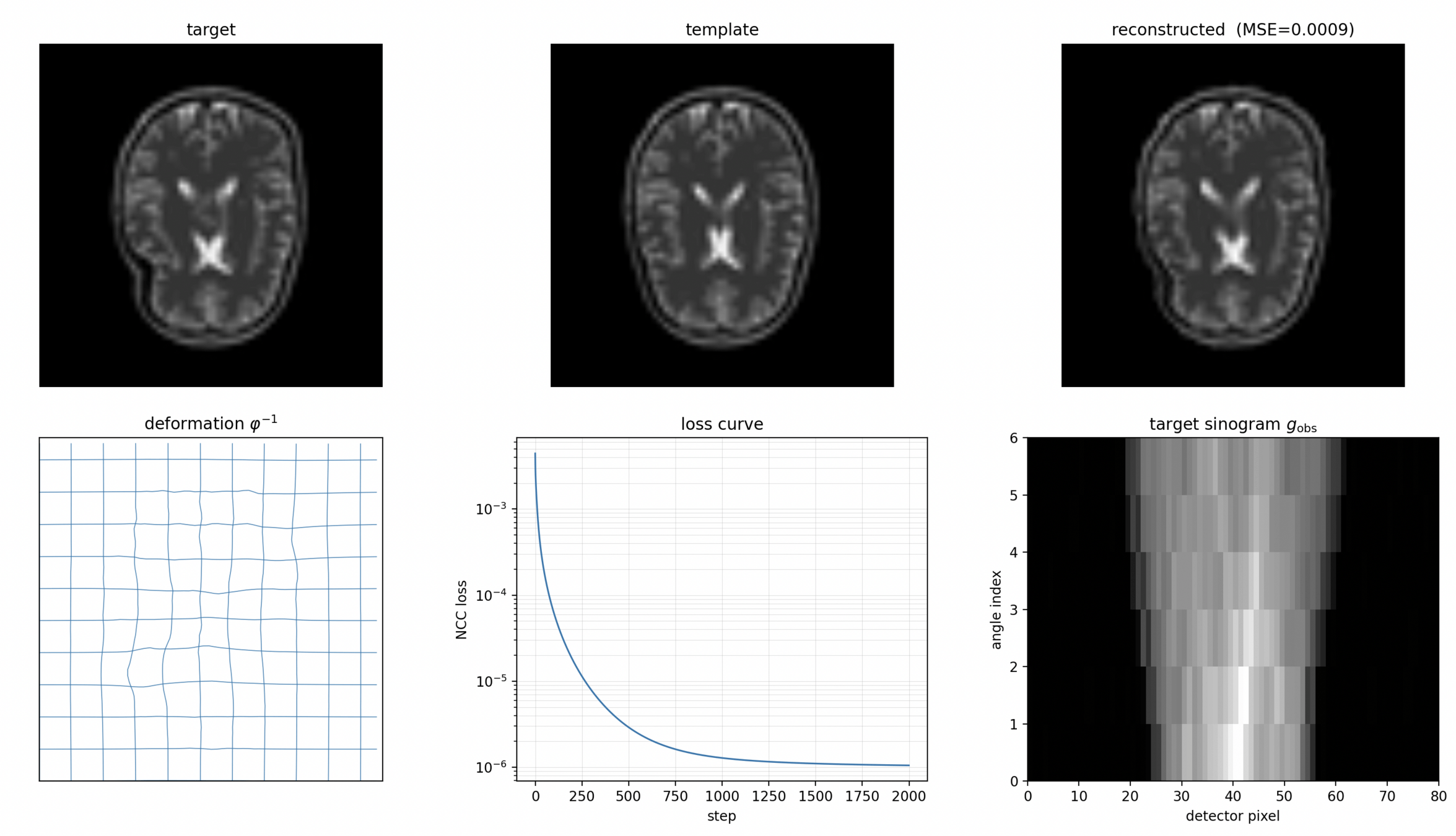
- Data fidelity is once again NCC \(\mathcal{L}_y(y')=1-\frac{\langle y,y'\rangle}{\|y\| \|y'\|}\)
Momentum map of action \(\Phi(g,w) = w\circ g^{-1}\)
Tomography gradient flow
The unregularized gradient flow is given by:
How and why to regularize?
Tomography results
Observations
Reconstruction
Target
Runs in a few seconds (but quite small images)
Tomography results
But now turn up the noise... (a factor 100, so not super realistic)
Reconstruction quality starts to deterioriate!
Two approaches to regularization
- Set \(V_R = \operatorname{Dens}(M)\): Regularization by action of \(g\) on reference volume, \(\Phi_R(g, \mathrm{d}x) = |Dg^{-1}|\mathrm{d}x\)
Recovers regularization part of a gradient flow from Bauer et al.
- Set \(V_R = \operatorname{Met}(M)\): Regularization by action of \(g\) on reference metric \(\mathbf{h}\), \(\Phi_R(g, \mathbf{h}) =\mathbf{h}_{g^{-1}(x)} (dg^{-1}u,dg^{-1}v)\)
Recovers regularization part of a gradient flow from Balehowsky et al.
Two approaches to regularization
Extend shape space and re-apply momentum map (which now is a sum)
Big question for me: Well-posedness.
For example, in tomography, pseudodifferential operators inside the GF appears.
Bit messy, but maybe Ebin–Marsden saves the day?
In summary
Fast and easy to converge
Comparable reconstructions to LDDMM
Easy to regularize
(but this is a story for another time)