Artificial neural networks for neuroscience
Erin Grant
Gatsby Unit & SWC, UCL
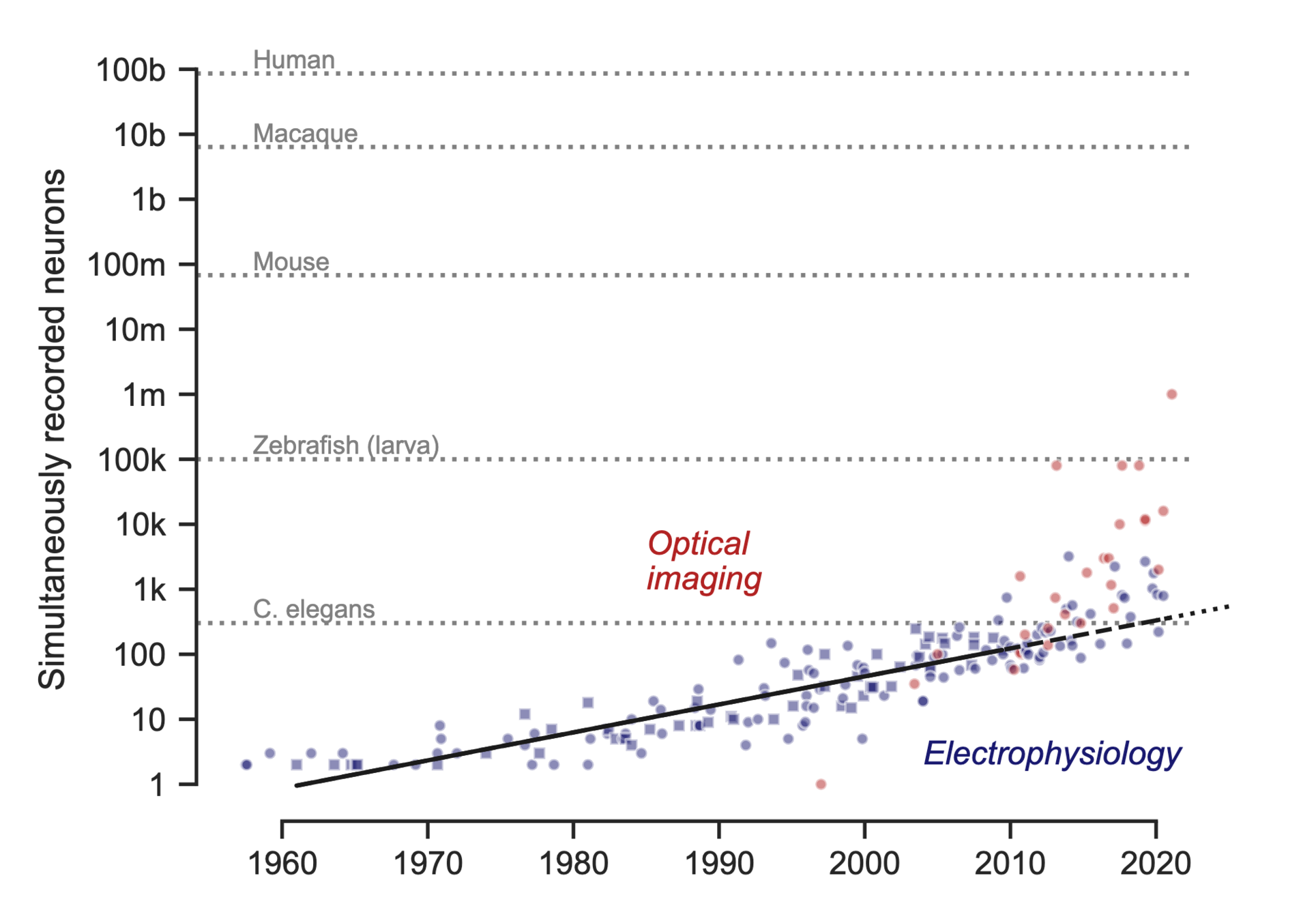
SWC Neuroinformatics 2024Improving techniques for recording population activity
Interpreting (lots of) neural data
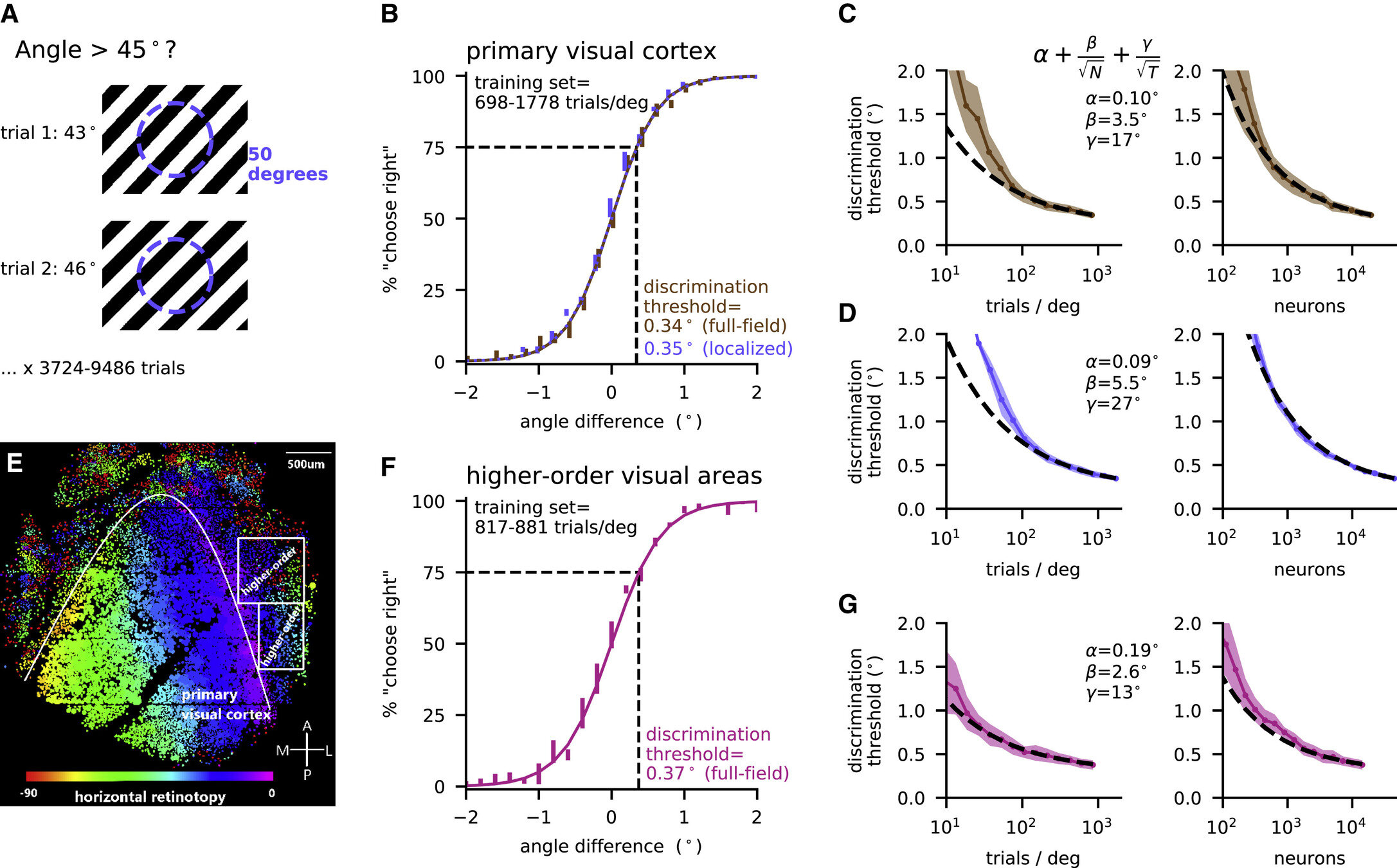
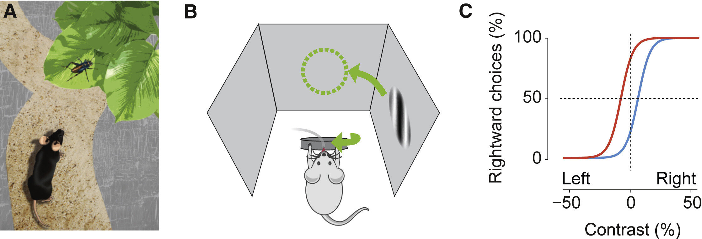
Canonical task: Orientation discrimination
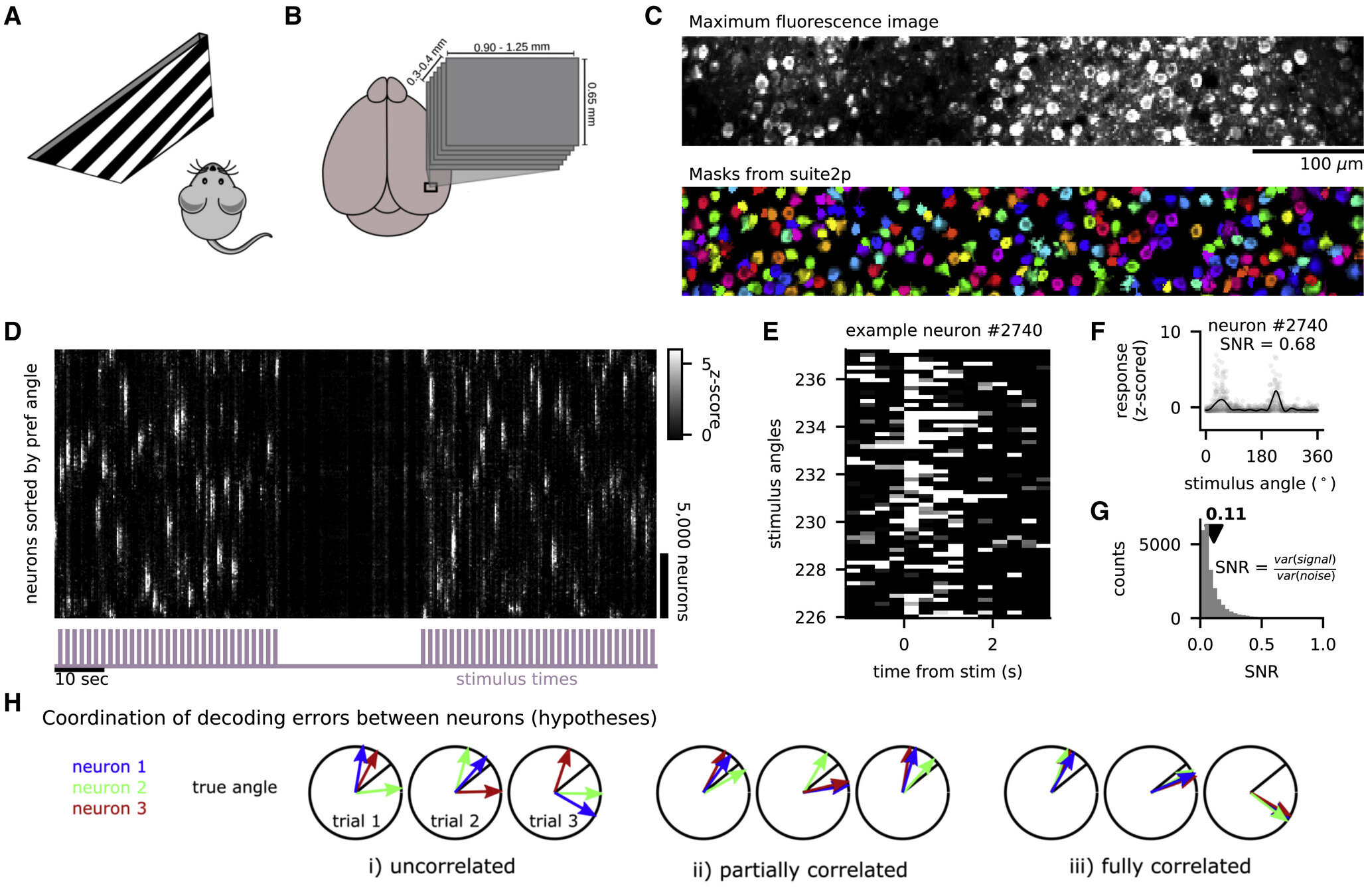
head-fixed mouse
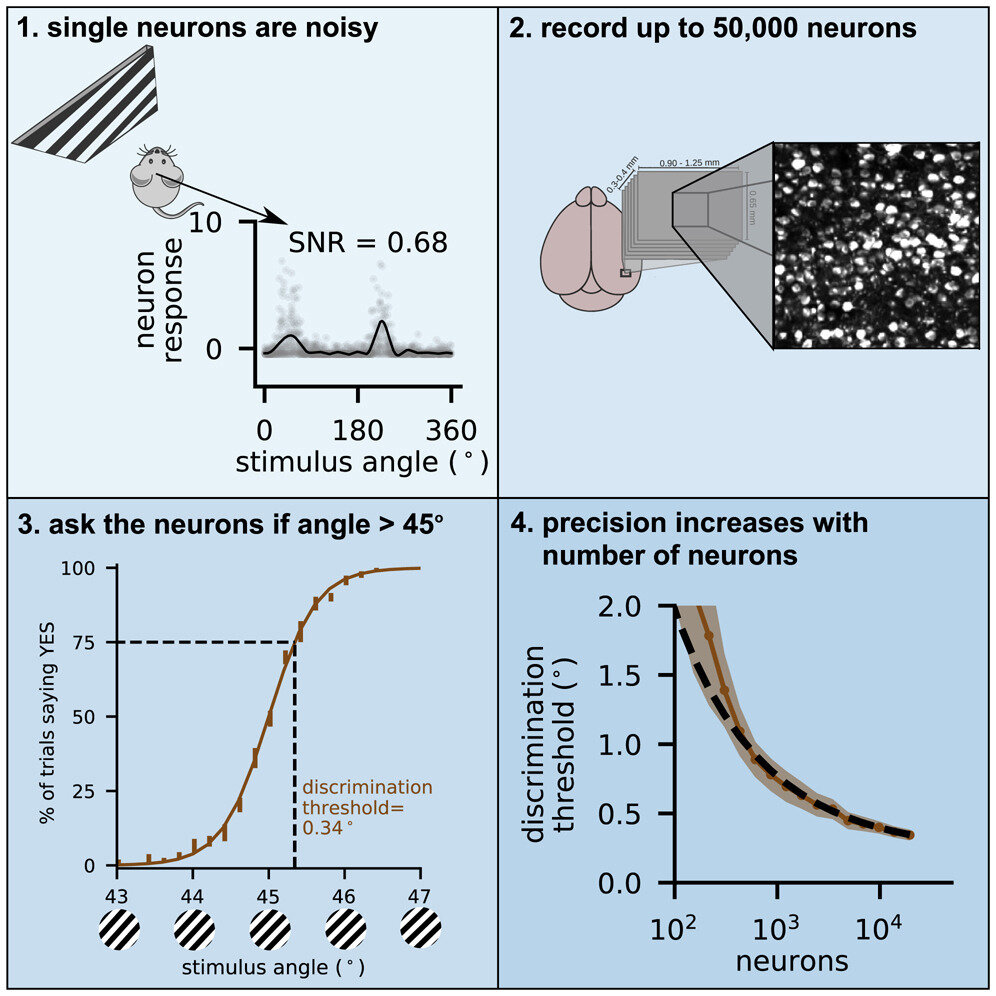
image 50K neurons
single neuron activity

decode "angle > 45
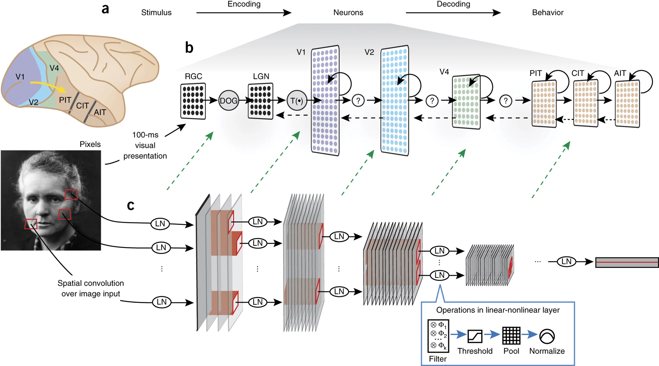
Modelling paradigms
Encoding:
Decoding:
Reverse-engineering:
Modelling paradigms
Reverse-engineering:
ANNs: Micro-scale
a single unit ("neuron"), linear:
$$\hat{y}=b + \sum_i w_i x_i $$
ANNs : Micro-scale
preactivation: $$ z=b+\sum_i w_i x_i $$
activation function:
$$g(z)=\max (0, z)$$
postactivation: $$ h= g(b+\sum_i w_i x_i )$$
Activation functions
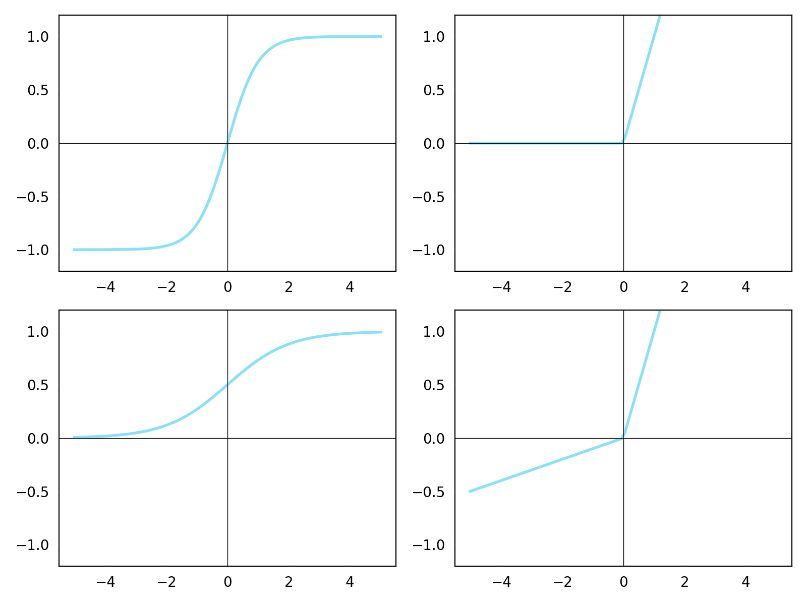
$$g(z)=\tanh(z)$$
$$g(z)=\max(0, z)$$
$$g(z)=\frac{1} {1 + e^{-x}}$$
$$g(z)=\max(\alpha z, z)$$
hyperbolic tangent
sigmoid
rectified linear (ReLU)
leaky ReLU
ANNs: Meso-scale
ANNs: Meso-scale
a single layer
(collection of neurons):
$$ \mathbf{h}=g(\mathbf{W}\mathbf{x})$$
ANNs: Meso-scale
a deep net
(sequence of layers):
$$\mathbf{h}^{(\ell)} = g(\mathbf{W}^{(\ell)}\mathbf{h}^{(\ell-1)})$$
$$\mathbf{h}^{(0)} = \mathbf{x}$$
$$\hat{\mathbf{y}} = \mathbf{W}^{(L)}\mathbf{h}^{(L-1)}$$
ANNs: Macro-scale
feedforward net
multi-layer perceptron
multi-layer perceptron
...anything that can be topologically ordered!
(all DAGs)
convolutional net
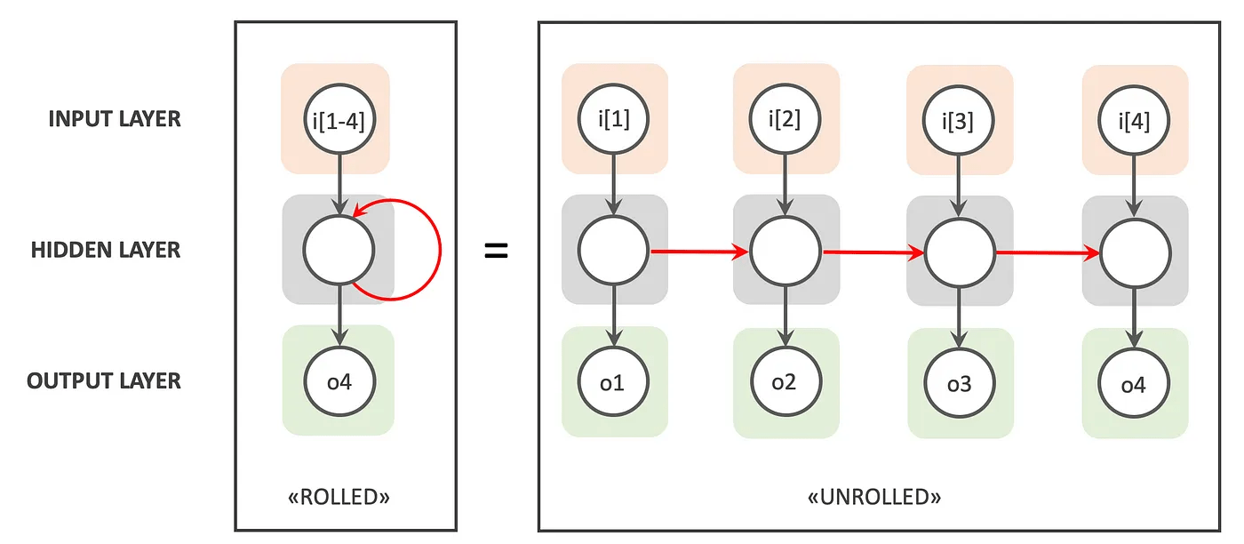
recurrent net
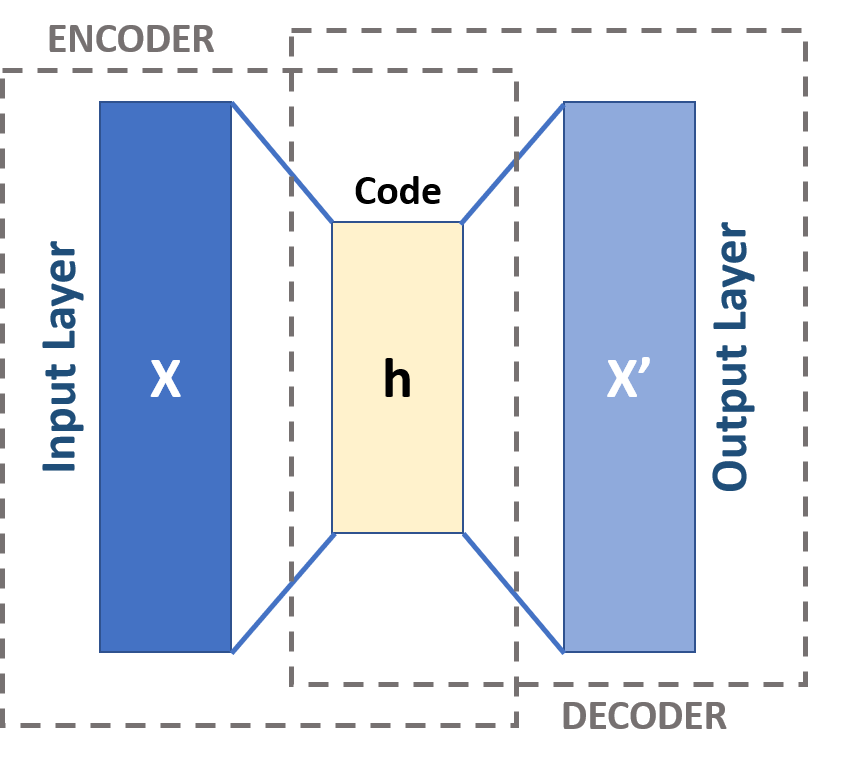
autoencoder
Loss functions
ground truth input
reconstructed input
("surrogate loss")
ground truth target
predicted target
intermediate representation
mean squared error (MSE)
usually for regression
cross entropy (xent)
usually for classification
supervised
unsupervised
(L2) reconstruction error
usually for an autoencoder
contrastive loss
usually for self-supervised learning
Training an ANN
Loss function for each datapoint:
$$\ell ( \hat{y}, y)=\cfrac{1}{2}(y- \hat{y})^2$$
Training corresponds to searching for a minimum:$$\arg\min_{w_1, w_2} \mathcal{L}(w_1, w_2)$$
$$\mathcal{L}(w_1, w_2) = \frac{1}{N} \sum_{i=1}^N \ell (\hat{y_i}, y_i)$$
Let's consider the average loss across N training examples as a function of the weights:
$$\hat{y}=w_1 x_1 + w_2 x_2$$
(equivalent to linear regression!)
The loss landscape view
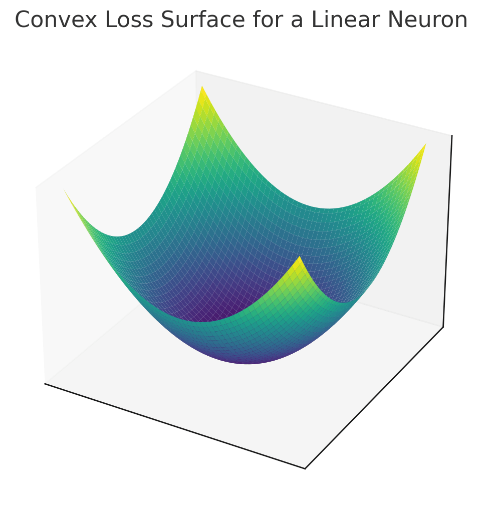
linear neuron, MSE
$$\mathcal{L}(w_1, w_2)$$
deep neural network
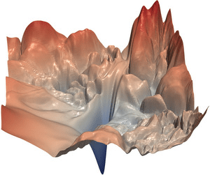
deep neural network
(low-D projection)
$$\mathcal{L}(\mathbf{W}^{(1)}, \mathbf{W}^{(2)}, \dots)$$
Idea: Pick a starting point. Use local information about the loss function to decide where to move next.
Iterative optimization
The best local information is usually the direction of steepest decrease of the loss, equivalent to the negative of the gradient:
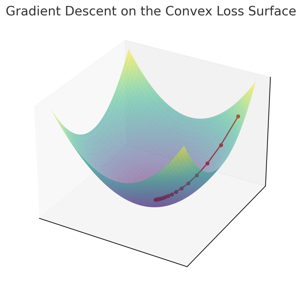
$$\mathcal{L}(w_1, w_2)$$
Convexity
Think: A ball rolled from any point on the loss surface will find its way to the lowest possible height.
A sufficient condition for all minima to be global minima.
i.e., if minima exist (the loss is bounded below), then all minima are equally good.
(Or will roll to negative infinity!)
$$\mathcal{L}(w_1, w_2)$$
Nonconvexity
(strictly) convex → unique global minimum
$$\mathcal{L}(w_1, w_2)$$
$$\mathcal{L}(\mathbf{W}^{(1)}, \mathbf{W}^{(2)}, \dots)$$
nonconvex
→
local minima, saddle points, plateaux, ravines
(possible but not guaranteed)
Nonlinearity
What can't we do with a linear neuron?
No linear decision boundary can separate the purple and yellow classes!
(Impossible to find weights for the linear neuron that achieve low error.)
exclusive OR (XOR)
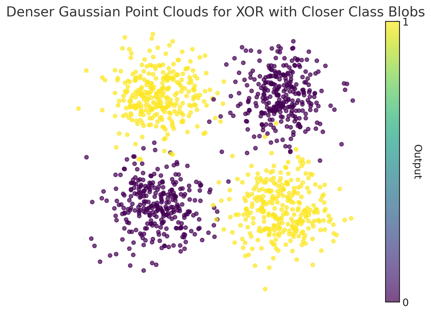
Nonlinearity
Adding just one multiplicative feature makes the problem linearly separable;
i.e., with this augmented "dataset", we can find weights that enable a linear neuron to solve the task.
Neural networks automate this process of feature learning!
Optimization in deep nets
Recall: steepest descent follows the negative direction of the gradient.
and similarly for the other weight.
$$\nabla \mathcal{L}(\mathbf{W}^{(1)}, \mathbf{W}^{(2)}, \dots)$$
is very complex! Can we do better than chain rule for every weight?
Backpropagaton
forward pass:
(compute loss)
backward pass:
(propagate error signal)
This procedure generalizes to all ANNs because they are DAGs!
$$\tfrac{\partial \ell}{\partial \ell}=1$$
$$\tfrac{\partial \ell}{\partial \hat{\mathbf{y}}}=\tfrac{\partial \ell}{\partial \ell} (\mathbf{y} - \hat{\mathbf{y}})$$
$$\tfrac{\partial \ell}{\partial \mathbf{W}^{(2)}}=\tfrac{\partial \ell}{\partial \hat{\mathbf{y}}} \mathbf{h}^T$$
$$\tfrac{\partial \ell}{\partial \mathbf{h}}={\mathbf{W}^{(2)}}^T \tfrac{\partial \ell}{\partial \mathbf{y}}$$
$$\tfrac{\partial \ell}{\partial \mathbf{z}}=\tfrac{\partial \ell}{\partial \mathbf{h}} \cdot g'(\mathbf{z})$$
$$\tfrac{\partial \ell}{\partial \mathbf{W}^{(1)}}=\tfrac{\partial \ell}{\partial \mathbf{z}} \mathbf{x}^T$$
$$\mathbf{z} = \mathbf{W}^{(1)}\mathbf{x}$$
$$\hat{\mathbf{y}} = \mathbf{W}^{(2)}\mathbf{h}$$
$$\mathbf{h} = g(\mathbf{z})$$
$$\ell=\tfrac{1}{2}\|\mathbf{y}-\hat{\mathbf{y}}\|^2$$
Open directions
Neural networks are a normative model:
They produce behavior and neural activity that is similar to biological intelligence when trained in an ecological task setting.
But the architectures, not to mention the neurons, as well as the learning rules are not biologically plausible.
We can still:
- Study how neural networks learn to perform tasks, and whether it is similar to how biological systems solve the same problem or not.
- Make quantitative predictions about interventions on activations & weights.
- Make quantitative predictions about generalization to new stimuli, tasks, etc.
Architectural manipulations motivated by biological plausibility.
Hypotheses in neural predictivity
hierarchical convolutional structure
local and long-range recurrence

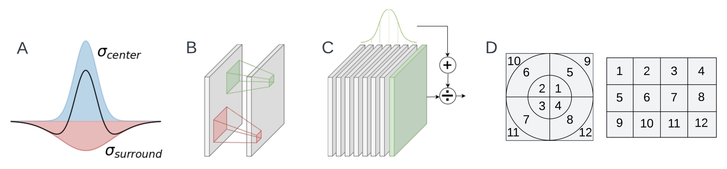
Manipulations don't always confer neural predictivity
