ML for physical and natural scientists 2023 2
dr.federica bianco | fbb.space | fedhere | fedhere

II probability and statistics
Week 1: Probability and statistics (stats for hackers)
Week 2: linear regression - uncertainties
Week 3: unsupervised learning - clustering
Week 4: kNN | CART (trees)
Week 5: Neural Networks - basics
Week 6: CNNs
Week 7: Autoencoders
Week 8: Physically motivated NN | Transformers
Somewhere I will also cover:
notes on visualizations
notes on data ethics
Tuesday: "theory"
Thursday: "hands on work"
Friday: "recap and preview"
slido.com
#2492 113

github

Reproducible research means:
all numbers in a data analysis can be recalculated exactly (down to stochastic variables!) using the code and raw data provided by the analyst.
Claerbout, J. 1990,
Active Documents and Reproducible Results, Stanford Exploration Project Report, 67, 139
reproducibility
allows reproducibility through code distribution
github
the Git software
is a distributed version control system:
a version of the files on your local computer is made also available at a central server.
The history of the files is saved remotely so that any version (that was checked in) is retrievable.
version control
allows version control
github
collaboration tool
by fork, fork and pull request, or by working directly as a collaborator
collaborative platform
allows effective collaboration

Reproducibility
Reproducible research means:
the ability of a researcher to duplicate the results of a prior study using the same materials as were used by the original investigator. That is, a second researcher might use the same raw data to build the same analysis files and implement the same statistical analysis in an attempt to yield the same results.
- provide raw data and code to reduce it to all stages needed to get outputs
- provide code to reproduce all figures
- provide code to reproduce all number outcomes
- seed your code random variables
Reproducible research in practice:
using the code and raw data provided by the analyst.
all numbers in an analysis can be recalculated exactly (down to stochastic variables!)
Assignments rules
your data should be accessible e.g. reading in a URL; all data you use should be public
-> use public data with live links
-> put your data on github if not accessible
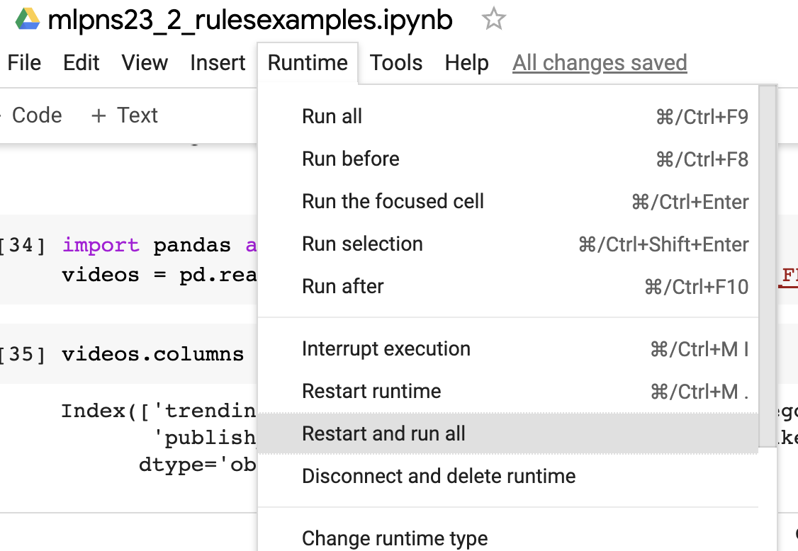
your notebook should work and reproduce exactly the results you reported in your notebook version
-> restart kernel + run all
->seed your code random variables

Assignments rules
your data should be accessible e.g. reading in a URL; all data you use should be public
-> use public data with live links
-> put your data on github if not accessible
your notebook should work and reproduce exactly the results you reported in your notebook version
-> restart kernel + run all
->seed your code random variables

Assignments rules
Other rules:
- Every figure should have axed labels
-
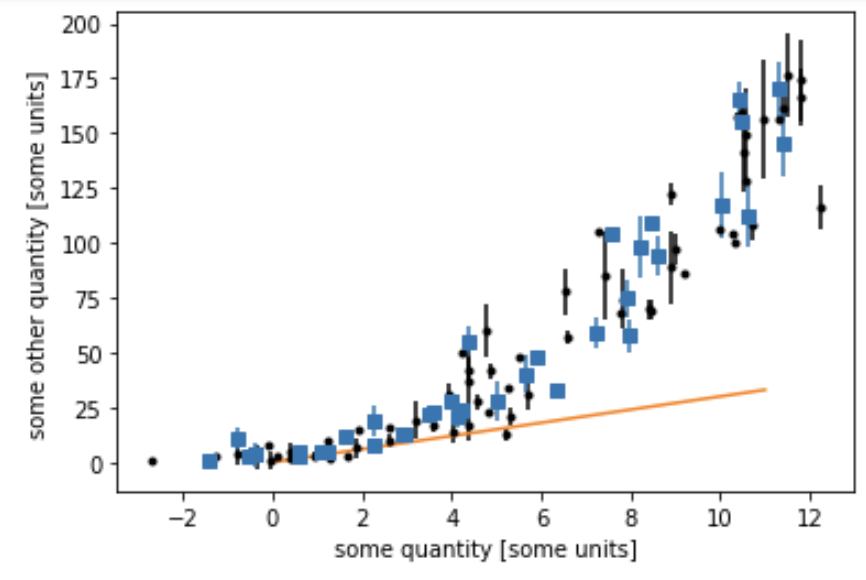
Every figure should have a caption that describes :
- what is being plotted (this plot shows ... against ... black dots are ... blue squares are... the line represents a linear model to...)
- why is interesting in the flow of your analysis (e.g. the model (orange line) is a good fit to the data only up to about x=4, at which point the data is systematically underpredicted by the model)
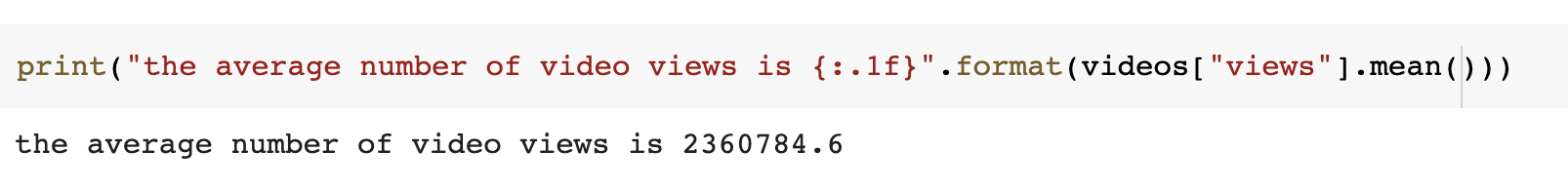
- The numbers that you print out should be explained. For example they should be embedded in a print statement (e.g. )
what are probability and statistics?
Crush Course in Statistics
freee statistics book: http://onlinestatbook.com/
Introduction to Statistics: An Interactive e-Book
probability
1
Basic Probability Frequentist interpretation
fraction of times something happens
probability of it happening
Basic Probability Bayesian interpretation
represents a level of certainty relating to a potential outcome or idea:
if I believe the coin is unfair (tricked) then even if I get a head and a tail I will still believe I am more likely to get heads than tails
<=>

Basic Probability Frequentist interpretation
fraction of times something happens
probability of it happening
<=>
P(E) = frequency of E
P(coin = head) = 6/11 = 0.55
Basic Probability Frequentist interpretation
fraction of times something happens
probability of it happening
<=>
P(coin = head) = 49/100 = 0.49
P(E) = frequency of E
P(coin = head) = 6/11 = 0.55

Basic probability arithmetics
Probability Arithmetic
disjoint events
A
B
Basic probability arithmetics
Probability Arithmetic
dependent events
A
B
Basic probability arithmetics
Probability Arithmetic
dependent events
A
B
Basic probability arithmetics
Probability Arithmetic
dependent events
statistics
2
statistics
takes us from observing a limited number of samples to infer on the population
TAXONOMY
Distribution: a formula (a model)
Population: all of the elemnts of a "family"
Sample: a finite subset of the population that you observe
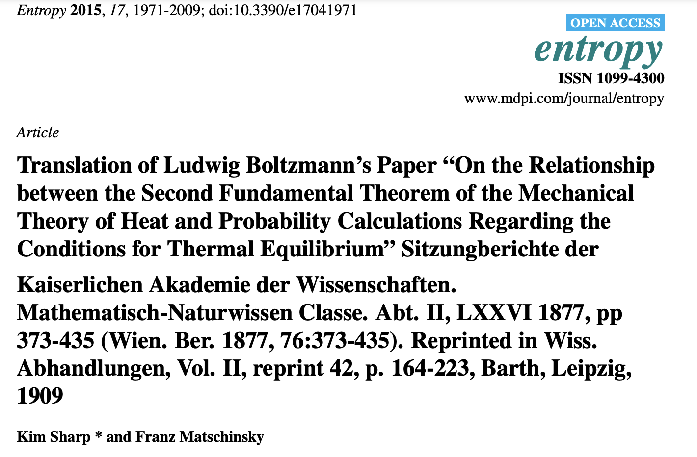
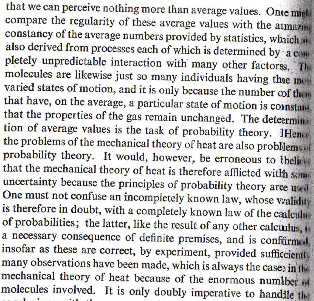
The application of stastistics to physics
Statistical Mechanics:
explains the properties of the macroscopic system by statiscal knowledge of the microscopic system, even the the state of each element of the system cannot be known exactly
Phsyics Example
describe properties of the Population while the population is too large to be observed.
Statistical Mechanics:
explains the properties of the macroscopic system by statiscal knowledge of the microscopic system, even the the state of each element of the system cannot be known exactly
example: Maxwell Boltzman distribution of velocity of molecules in an ideal gas
Phsyics Example
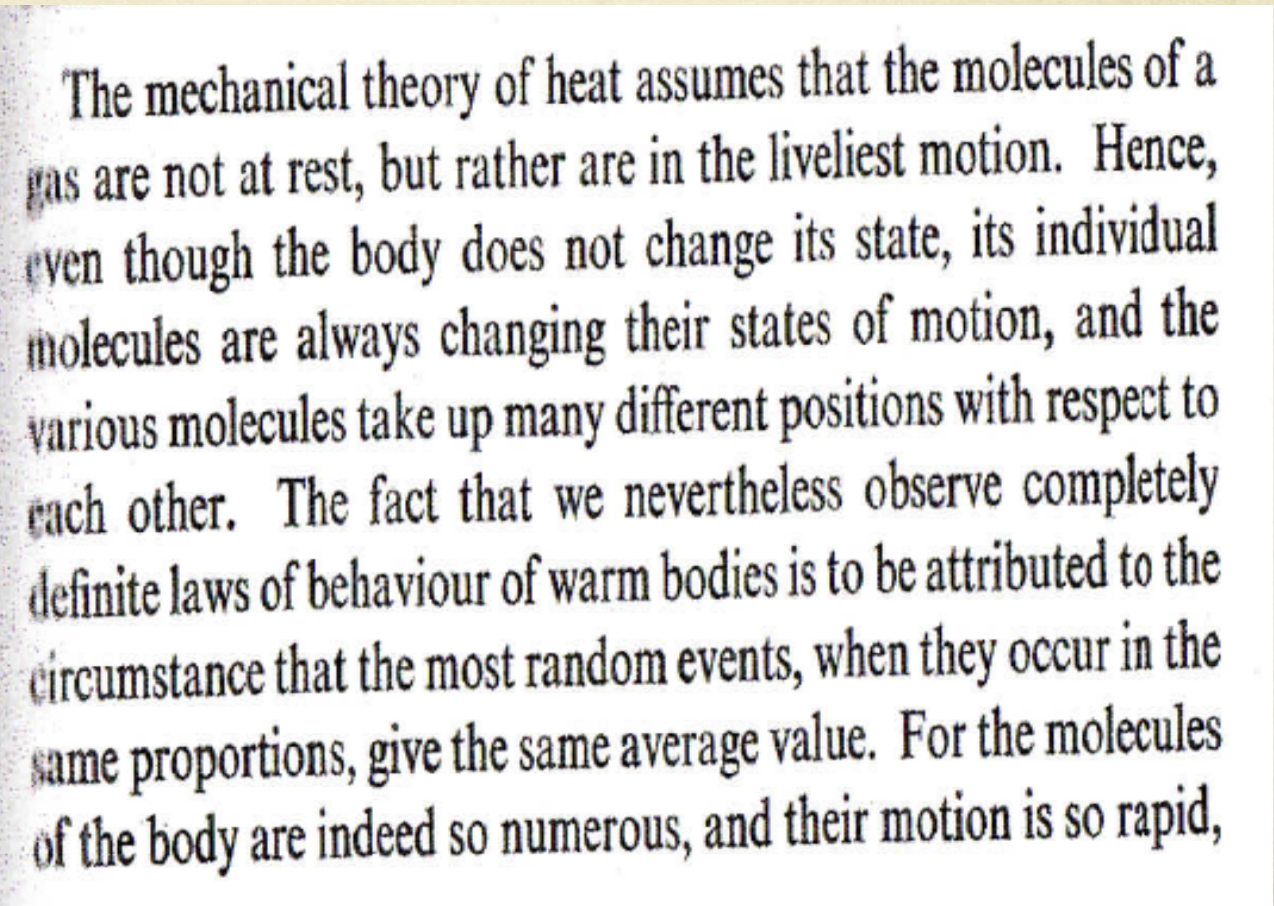
Boltzmann 1872
Phsyics Example
Boltzmann 1872
Boltzmann 1872
Phsyics Example
3
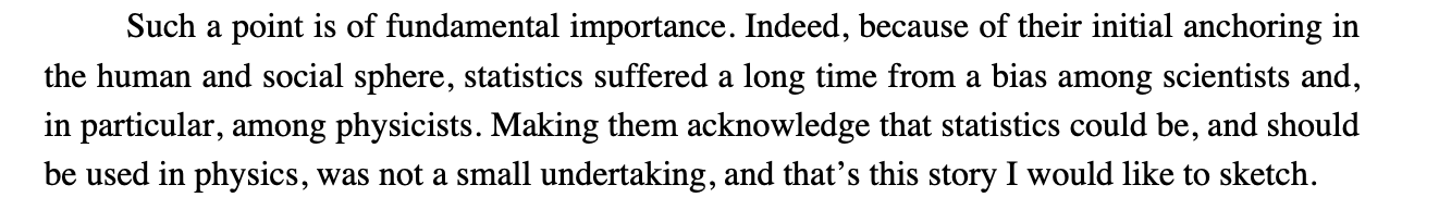
descriptive statistics:
we summarize the proprties of a distribution
descriptive statistics:
# myarray is a numpy array
myarray.mean() # the mean of all numbers in the array
myarray.mean(axis=1) # the mean along the second axis (one number per array row)
descriptive statistics:
we summarize the proprties of a distribution
mean: n=1
other measures of centeral tendency:
median: 50% of the distribution is to the left,
50% to the right
mode: most popular value in the distribution
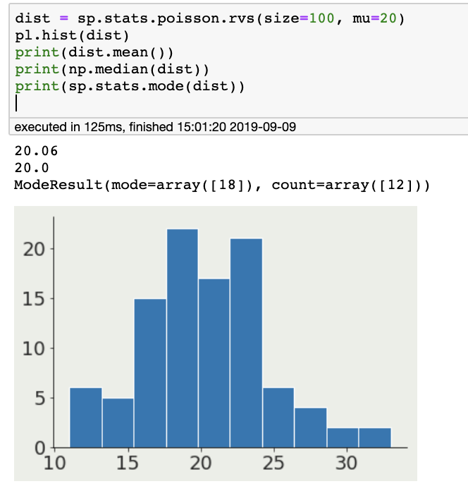
descriptive statistics:
we summarize the proprties of a distribution
variance: n=2
standard deviation
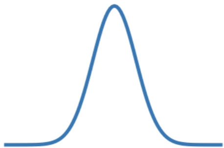
Gaussian distribution:
1σ contains 68% of the distribution
68%
# myarray is a numpy array
myarray.std() # the standard dev of all numbers in the array
myarray.std(axis=1) # the standard dev  along the second axis (one number per array row)
descriptive statistics:
we summarize the proprties of a distribution
variance: n=2
standard deviation
Gaussian distribution:
2σ contains 95% of the distribution
95%
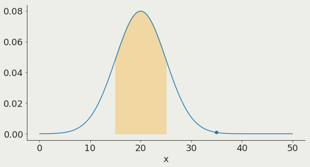
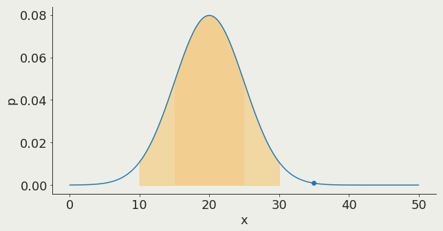
descriptive statistics:
we summarize the proprties of a distribution
variance: n=2
standard deviation
Gaussian distribution:
3σ contains 97.3% of the distribution
97.3%
TAXONOMY
central tendency: mean, median, mode
spread : variance, interquantile range
Probability distributions
Coin toss:
fair coin: p=0.5 n=1
Vegas coin: p=0.5 n=1
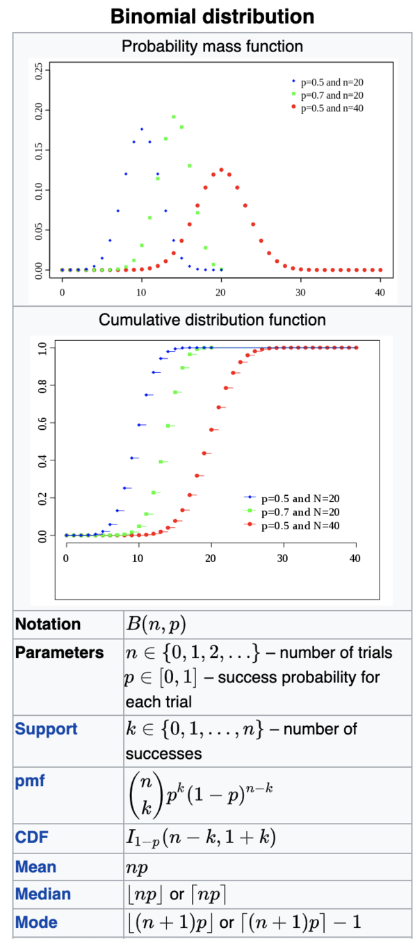
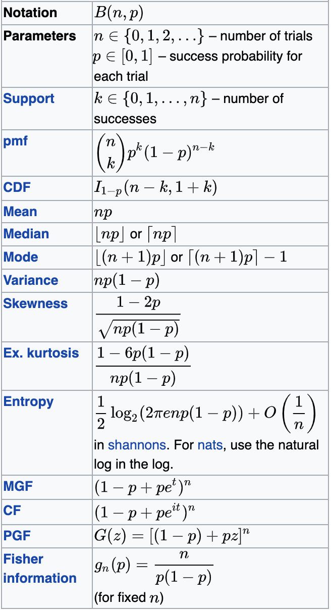
Binomial
Probability distributions
Coin toss:
fair coin: p=0.5 n=1
Vegas coin: p=0.5 n=1
Binomial
Probability distributions
Coin toss:
fair coin: p=0.5 n=1
Vegas coin: p=0.5 n=1
Binomial
Probability distributions
Coin toss:
fair coin: p=0.5 n=1
Vegas coin: p=0.5 n=1
Binomial
Probability distributions
central tendency
np=mean
Coin toss:
fair coin: p=0.5 n=1
Vegas coin: p=0.5 n=1
Binomial
Probability distributions
np(1-p)=variance
Binomial
Coin toss:
fair coin: p=0.5 n=1
Vegas coin: p=0.5 n=1
Probability distributions
Shut noise/count noise
The innate noise in natural steady state processes (star flux, rain drops...)
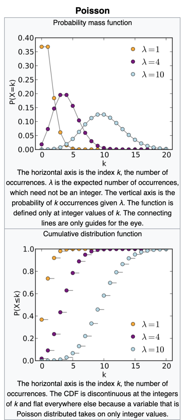
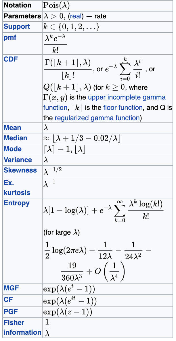
λ=mean
Poisson
Probability distributions
λ=variance
Shut noise/count noise
The innate noise in natural steady state processes (star flux, rain drops...)
Poisson
Probability distributions
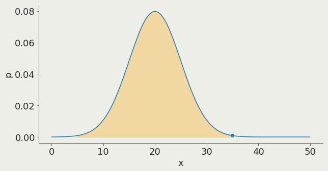
most common noise:
well behaved mathematically, symmetric, when we can we will assume our uncertainties are Gaussian distributed
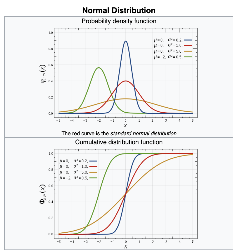
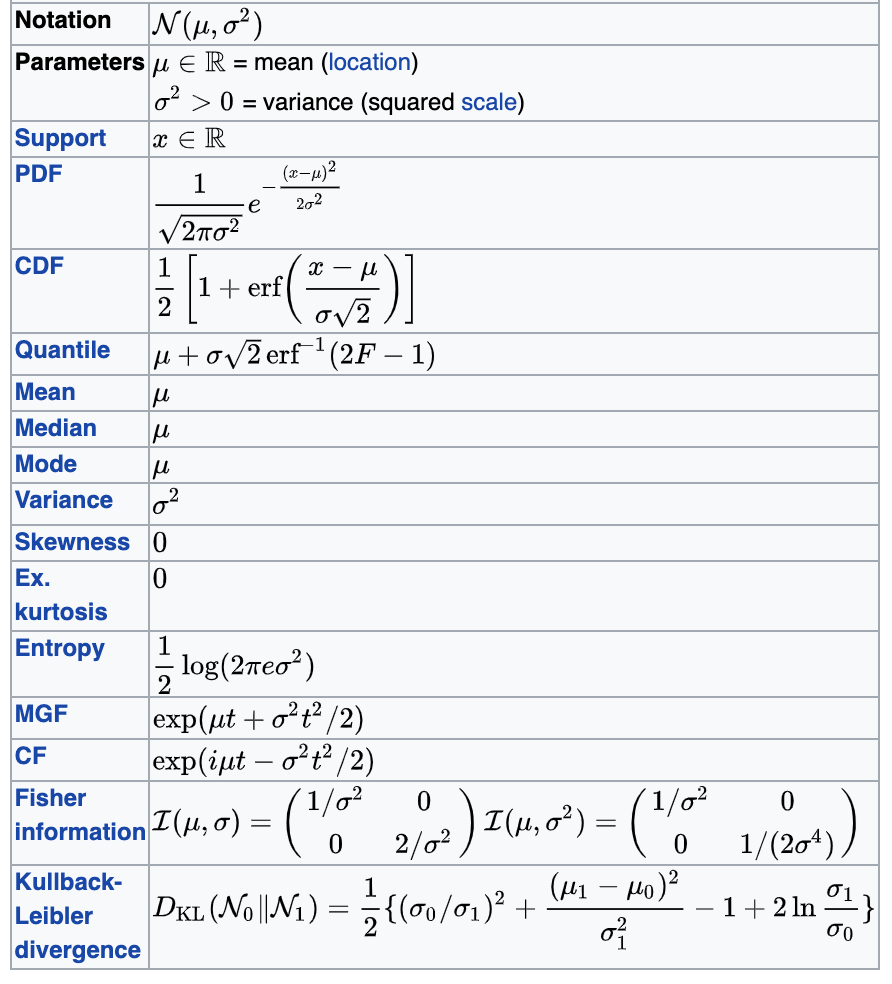
Gaussian
Probability distributions
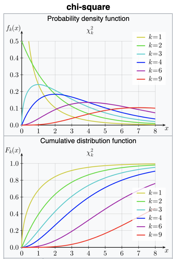
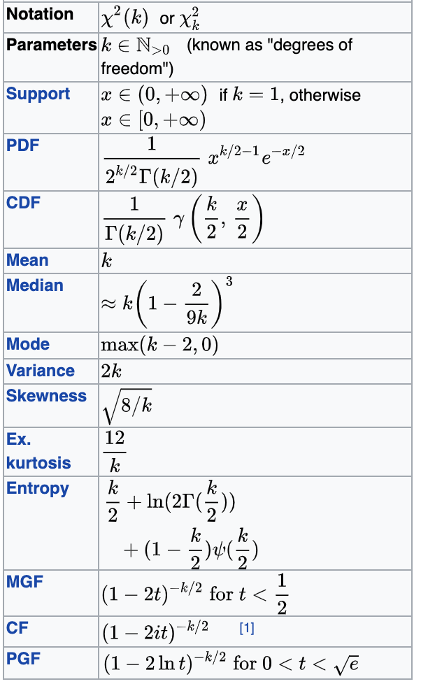
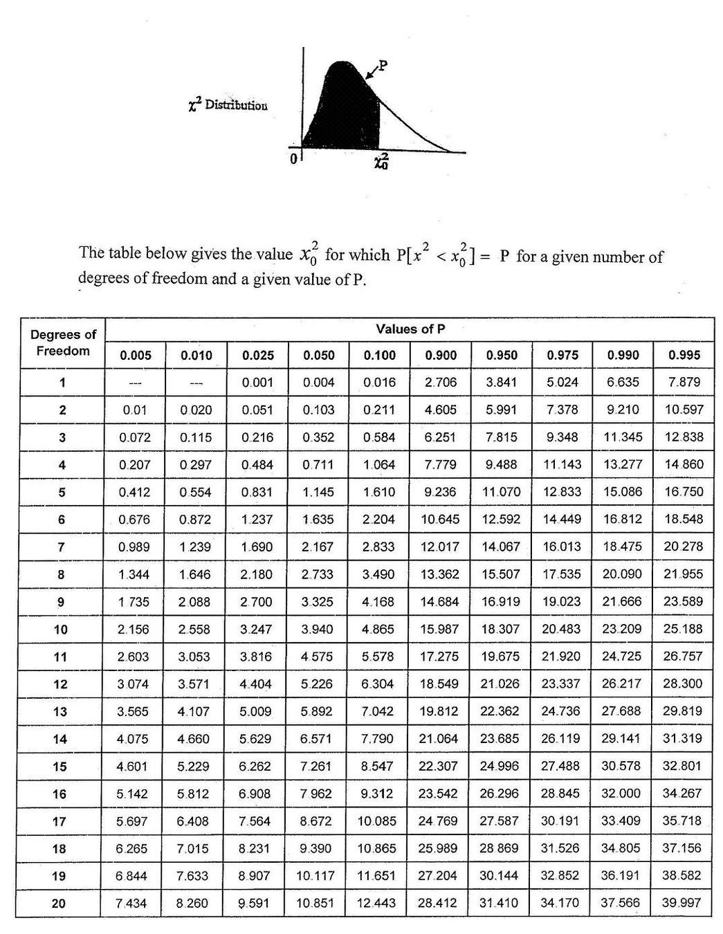
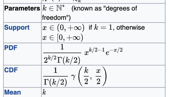
Chi-square (χ2)
turns out its extremely common
many pivotal quantities follow this distribution and thus many tests are based on this
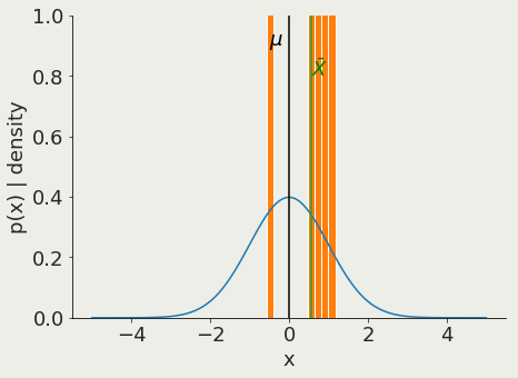
Suppose X1, X2, . . . , Xn are independent and identically-distributed, or i.i.d (=independent random variables with the same underlying distribution).
=>Xi all have the same mean µ and standard deviation σ.
Let X be the mean of Xi
Note that X is itself a random variable.
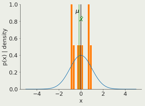
As Ν grows, the probability that X is close to µ goes to 1.
In the limit of N -> infinity
the mean of a sample of size Ν approaches the mean of the population μ
Law of large numbers
Laplace (1700s) but also: Poisson, Bessel, Dirichlet, Cauchy, Ellis
Let X1...XN be an N-elements sample from a population whose distribution has
mean μ and standard deviation σ
In the limit of N -> infinity
the sample mean x approaches a Normal (Gaussian) distribution with mean μ and standard deviation σ
regardless of the distribution of X
Central Limit Theorem
coding time!

key concepts
interpretation of probability
distributions
central limit theorem
homework
- HW1 : explore the Maxwell Boltzmann distribution
- HW2: graphic demonstration of the Central Limit Theorem
Foundations of Statistical Mechanics 1845—1915
Stephen G. Brush
Archive for History of Exact Sciences Vol. 4, No. 3 (4.10.1967), pp. 145-183
reading
resources
Sarah Boslaugh, Dr. Paul Andrew Watters, 2008
Statistics in a Nutshell (Chapters 3,4,5)
https://books.google.com/books/about/Statistics_in_a_Nutshell.html?id=ZnhgO65Pyl4C
David M. Lane et al.
Introduction to Statistics (XVIII)
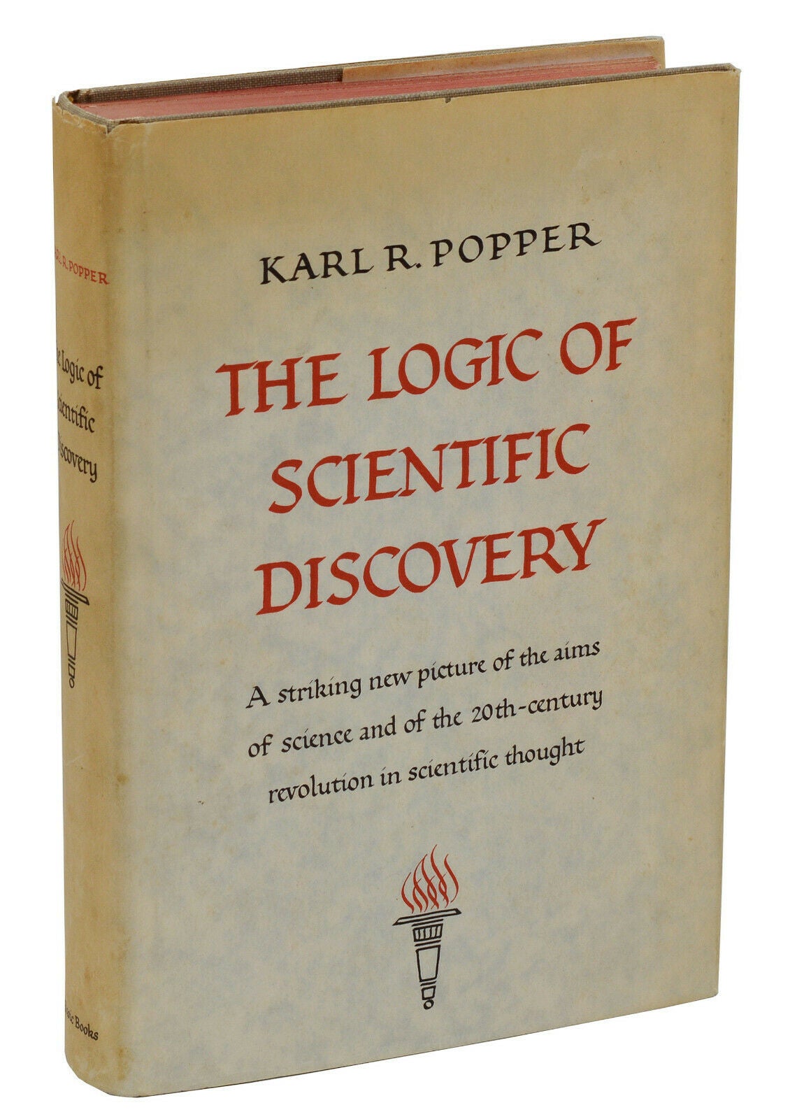
a scientific theory must be falsifiable
My proposal is based upon an asymmetry between verifiability and falsifiability; an asymmetry which results from the logical form of universal statements. For these are never derivable from singular statements, but can be contradicted by singular statements.
—Karl Popper, The Logic of Scientific Discovery
the demarcation problem:
what is science? what is not?
the scientific method
in a probabilistic context
4
p(physics | data)
https://speakerdeck.com/dfm/emcee-odi
p(physics | data)
https://speakerdeck.com/dfm/emcee-odi
Bayesian Inference
Forward Modeling
Frequentist approach (NHRT)
p(physics | data)
https://speakerdeck.com/dfm/emcee-odi
Null
Hypothesis
Rejection
Testing

model
prediction
data
does not falsify
falsifies
model
still holds
model
rejected
data
does not falsify
falsifies
model
prediction
model
still holds
"Under the Hypothesis" = if the model is true
model
rejected
data
does not falsify
falsifies
this will happen
model
prediction
model
still holds
model
rejected
"Under the Hypothesis" = if the model is true
data
does not falsify
falsifies
this has a low probability of happening
model
prediction
model
still holds
model
rejected
"Under the Null Hypothesis" = if the NH model is true
data
does not falsify
falsifies
model
prediction
model
still holds
low probability event happened
model
rejected
this has a low probability of happening
"Under the Null Hypothesis" = if the model is true
data
does not falsify
falsifies
model
still holds
rejected at 95%
0.05 p-value
5% confidence
low probability event happened
model
rejected
data
does not falsify
falsifies
model
still holds
rejected at 99.7%
0.003 p-value
0.3% confidence
low probability event happened
model
rejected
data
does not falsify
falsifies
model
still holds
rejected at 99.99...%
3-e7 p-value
3-e5% confidence
low probability event happened
model
rejected
data
does not falsify alternative
falsifies alternative
model still holds
"Under the Null Hypothesis" = if the proposed model is false
this has a low probability of happening
model
prediction
model rejected
low probability event happened
formulate the Null as the comprehensive opposite of your theory
Null hyposthesis rejection testing
5
Null
Hypothesis
Rejection
Testing
formulate your prediction
Null Hypothesis
1
Null
Hypothesis
Rejection
Testing
Alternative Hypothesis
identify all alternative outcomes
2
Null
Hypothesis
Rejection
Testing
Alternative Hypothesis
2
if all alternatives to our model are ruled out, then our model must hold
identify all alternative outcomes
Null
Hypothesis
Rejection
Testing
Alternative Hypothesis
identify all alternative outcomes
2
if all alternatives to our model are ruled out, then our model must hold
same concept guides prosecutorial justice
guilty beyond reasonable doubt

data
does not falsify
falsifies
this has a low probability of happening
model
prediction
Null still holds
Null rejected
"Under the Null Hypothesis" = if the old model is true
But instead of verifying a theory we want to falsify one
generally, our model about how the world works is the Alternative and we try to reject the non-innovative thinking as the Null
data
does not falsify
falsifies
this has a low probability of happening
model
prediction
Null still holds
Null rejected
"Under the Null Hypothesis" = if the old model is true
But instead of verifying a theory we want to falsify one
Earth is flat is Null
Earth is round is Alternative:
we reject the Null hypothesis that the Earth is flat (p=0.05)
data
does not falsify
falsifies
this has a low probability of happening
model
prediction
Null still holds
Null rejected
"Under the Null Hypothesis" = if the old model is true
But instead of verifying a theory we want to falsify one
Earth is flat is Null
Earth is round not flat is Alternative:
we reject the Null hypothesis that the Earth is flat (p=0.05)
Null
Hypothesis
Rejection
Testing
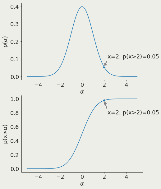
confidence level
p-value
threshold
3
set confidence threshold
95%
Null
Hypothesis
Rejection
Testing
4
find a measurable quantity which under the Null has a known distribution
pivotal quantities
pivotal quantities
quantities that under the Null Hypotheis follow a known distribution
if a quantity follows a known distribution, once I measure its value I can what the probability of getting that value actually is! was it a likely or an unlikely draw?
Null
Hypothesis
Rejection
Testing
4
pivotal quantities
quantities that under the Null Hypotheis follow a known distribution
also called "statistics"
e.g.: χ2 statistics: difference between expetation and reality squared
Z statistics: difference between means
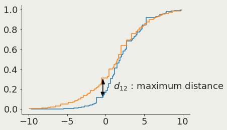
K-S statistics: maximum distance of cumulative distributions.
Null
Hypothesis
Rejection
Testing
4
pivotal quantities
quantities that under the Null Hypotheis follow a known distribution
Null
Hypothesis
Rejection
Testing
4
Null
Hypothesis
Rejection
Testing
5
calculate it!
pivotal quantities
Null
Hypothesis
Rejection
Testing
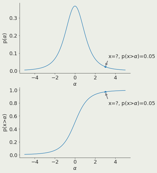
6
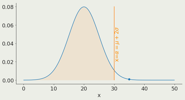
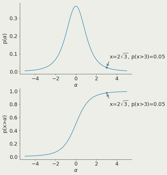
test data against alternative outcomes
95%
α is the x value corresponding to a chosen threshold
Null
Hypothesis
Rejection
Testing
6
test data against alternative outcomes
prediction is unlikely
Null rejected
Alternative holds
Null
Hypothesis
Rejection
Testing
6
test data against alternative outcomes
prediction is likely
Null holds
Alternative rejected
prediction is unlikely
Null rejected
Alternative holds
95%
Null
Hypothesis
Rejection
Testing
6
test data against alternative outcomes
prediction is likely
Null holds
Alternative rejected
prediction is unlikely
Null rejected
Alternative holds
95%
data
does not falsify alternative
falsifies alternative
model
holds
"Under the Null Hypothesis" = if the model is false
this has a low probability of happening
model
prediction
everything but model is rejected
low probability event happened
formulate the Null as the comprehensive opposite of your theory
Key Slide
formulate your prediction (NH)
1
2
identify all alternative outcomes (AH)
3
set confidence threshold
(p-value)
4
find a measurable quantity which under the Null has a known distribution
(pivotal quantity)
5
6
calculate the pivotal quantity
calculate probability of value obtained for the pivotal quantity under the Null
if probability < p-value : reject Null
Key Slide
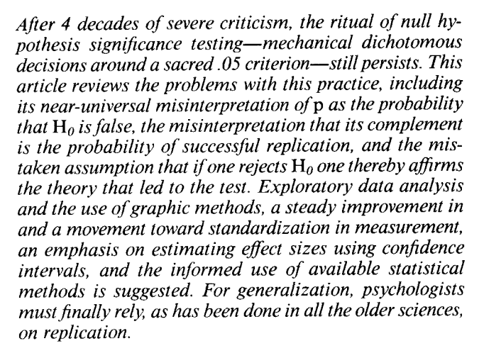
reading
the original link:
http://psycnet.apa.org/fulltext/1995-12080-001.html
(this link nees access to science magazine, but ou can use the link above which is the same file)
Jacob Cohen, 1994
The earth is round (p=0.05)

common tests and pivotal quantities
6
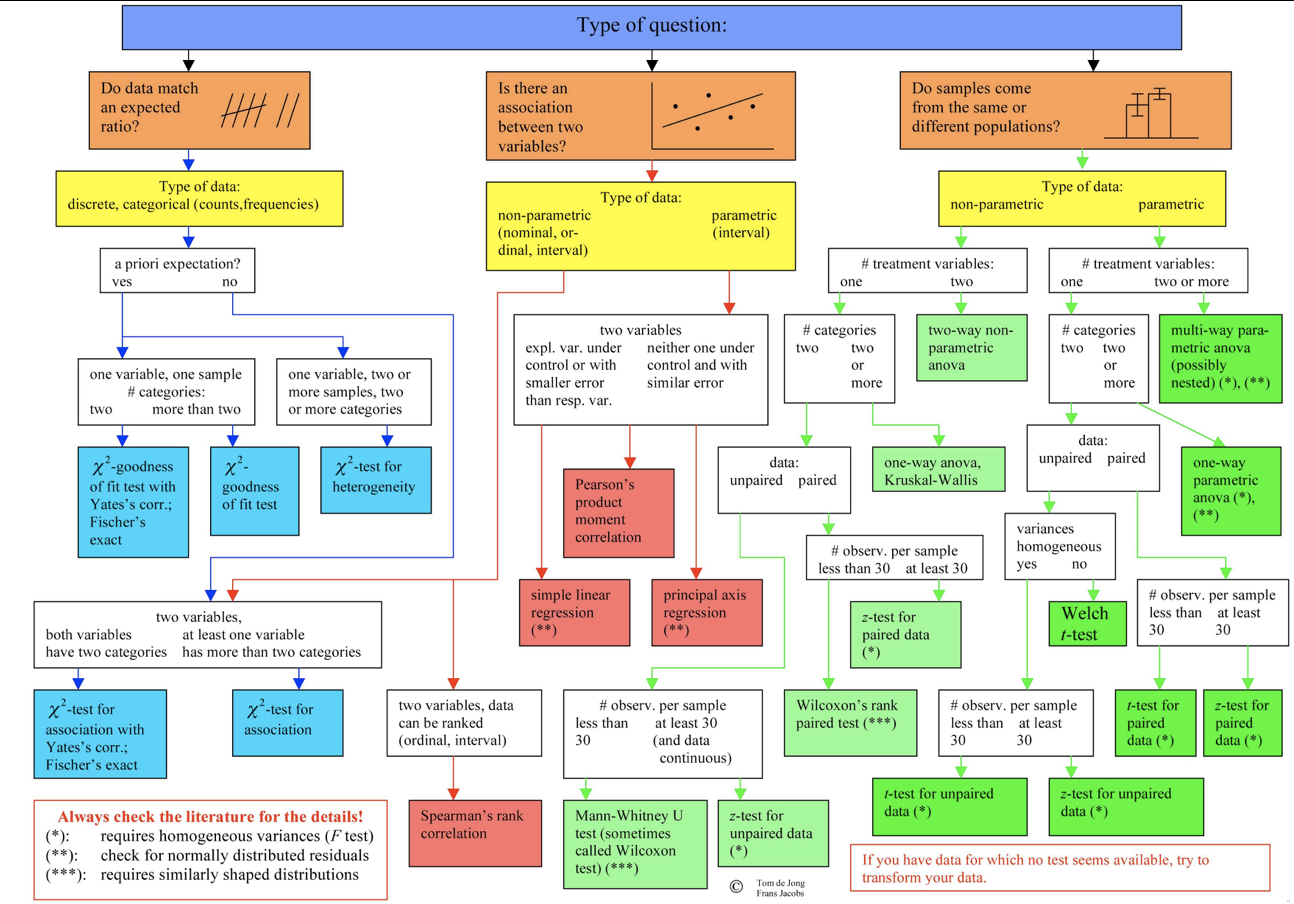
Z-test
Is the mean of a sample with known variance the same as that of a known population?
pivotal quantity
sample mean
sample variance =
population mean
Z-test
Is the mean of a sample with known variance the same as that of a known population?
pivotal quantity
sample mean
sample variance =
population mean
why do we need a test? why not just measuring the means and seeing it they are the same?
Z-test
Is the mean of a sample with known variance the same as that of a known population?
pivotal quantity
sample mean
population mean
sample variance =
Z-test
Is the mean of a sample with known variance the same as that of a known population?
pivotal quantity
sample mean
sample variance =
population mean
why should it depend on N? Law of large numbers
Z-test
Is the mean of a sample with known variance the same as that of a known population?
pivotal quantity
sample mean
sample variance =
population mean
The Z test provides a trivial interpretation of the measured quantity: the Z value is exactly the distance for the mean of the standard distribution of possible outcomes in units of standard deviation
so a result of 0.13 means we are 0.13 standard deviations to the mean (p>0.05)
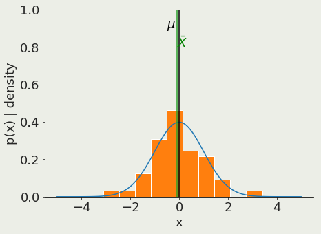
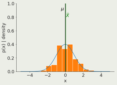
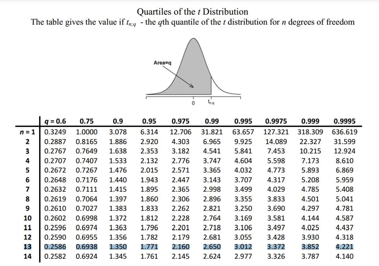
t- test
pivotal quantity
size of sample
unbias variance estimator
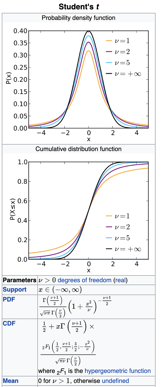


Are the means of 2 samples significantly different?
t- test
pivotal quantity
size of sample
unbias variance estimator
Are the means of 2 samples significantly different?
df=3
t- test
Are the means of 2 samples significantly different?
pivotal quantity
size of sample
unbias variance estimator
To interpret the outcome of a t-test I have to figure out the probability of a give p
so a result of 0.13 means we are 0.13 standard deviations to the mean (p>0.05)
t- test
Are the means of 2 samples significantly different?
pivotal quantity
size of sample
unbias variance estimator
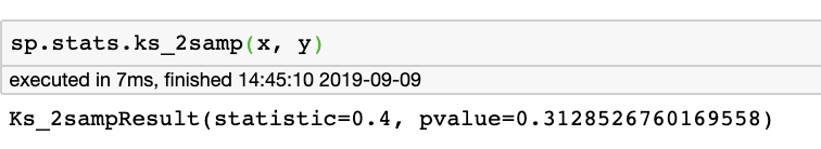
K-S test
Kolmogorof-Smirnoff :
do two samples come from the same parent distribution?
pivotal quantity
Cumulative distribution 1
Cumulative distribution 2
K-S test
Kolmogorof-Smirnoff :
do two samples come from the same parent distribution?
pivotal quantity
Cumulative distribution 1
Cumulative distribution 2
χ2 test
are the data what is expected from the model (if likelihood is Gaussian... we'll see this later) - ther are a few χ2 tests. The one here is the "Pearson's χ2 tests"
pivotal quantity
uncertainty
model
observation
number of observation
this should actually be the number of params in the model
χ2 test
pivotal quantity
uncertainty
model
observation
number of observation
are the data what is expected from the model (if likelihood is Gaussian... we'll see this later) - ther are a few χ2 tests. The one here is the "Pearson's χ2 tests"
the demarcation problem
in Bayesian context
beyond frequentism and NHRT
7
the demarcation problem
in Bayesian context
The probability that a belief is true given new evidence equals the probability that the belief is true regardless of that evidence times the probability that the evidence is true given that the belief is true divided by the probability that the evidence is true regardless of whether the belief is true.
- Thomas Bayes Essay towards solving a Problem in the Doctrine of Chances (1763)
"prior"
the demarcation problem
in Bayesian context
The probability that a belief is true given new evidence equals the probability that the belief is true regardless of that evidence times the probability that the evidence is true given that the belief is true divided by the probability that the evidence is true regardless of whether the belief is true.
- Thomas Bayes Essay towards solving a Problem in the Doctrine of Chances (1763)
"evidence"
pivotal quantities
quantities that under the Null Hypotheis follow a known distribution
Null
Hypothesis
Rejection
Testing
4
Bayes theorem
Bayes theorem
Bayes theorem
posterior
likelihood
prior
evidence
model parameters
data
D
Bayes theorem
constraints on the model
e.g. flux is never negative
P(f<0) = 0 P(f>=0) = 1
prior:
model parameters
data
D
Bayes theorem
model parameters
data
D
prior:
constraints on the model
people's weight <1000lb
& people's weight >0lb
P(w) ~ N(105lb, 90lb)
Bayes theorem
model parameters
data
D
prior:
constraints on the model
people's weight <1000lb
& people's weight >0lb
P(w) ~ N(105lb, 90lb)
the prior should not be 0 anywhere the probability might exist
Bayes theorem
model parameters
data
D
prior:
"uninformative prior"
Bayes theorem
likelihood:
this is our model
model parameters
data
D
Bayes theorem
evidence
????
model parameters
data
D
Bayes theorem
evidence
????
model parameters
data
D
it does not matter if I want to use this for model comparison
Bayes theorem
model parameters
data
D
it does not matter if I want to use this for model comparison
which has the highest posterior probability?
Bayes theorem
posterior: joint probability distributin of a parameter set (θ, e.g. (m, b)) condition upon some data D and a model hypothesys f
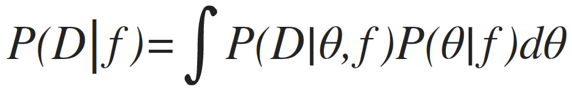
evidence: marginal likelihood of data under the model
prior: “intellectual” knowledge about the model parameters condition on a model hypothesys f. This should come from domain knowledge or knowledge of data that is not the dataset under examination
Bayes theorem
Bayes theorem
posterior: joint probability distributin of a parameter set (θ, e.g. (m, b)) condition upon some data D and a model hypothesys f
evidence: marginal likelihood of data under the model
prior: “intellectual” knowledge about the model parameters condition on a model hypothesys f. This should come from domain knowledge or knowledge of data that is not the dataset under examination
in reality all of these quantities are conditioned on the shape of the model: this is a model fitting, not a model selection methodology
the demarcation problem
in Bayesian context
The probability that a belief is true given new evidence equals the probability that the belief is true regardless of that evidence times the probability that the evidence is true given that the belief is true divided by the probability that the evidence is true regardless of whether the belief is true.
- Thomas Bayes Essay towards solving a Problem in the Doctrine of Chances (1763)
scaling laws
8
quantities that relate by powers
Example:
quantities that relate by powers
Example:
quantities that relate by powers
Example:
| scaling law: |
quantities that relate by powers
Example:
| scaling law: |
| scaling law: |
quantities that relate by powers
Example:
| scaling law: |
| scaling law: |
| regardless of the shape! |
quantities that relate by powers
Example:

quantities that relate by powers
Example:
why is this important?
The exsitance of a scaling relationship between physical quantities reveals an underlying driving mechanism
Astrophysics
The Tully–Fisher relation is an empirical relationship between the intrinsic luminosity of a spiral galaxy and its torational velocity
R. Brent Tully and J. Richard Fisher, 1977
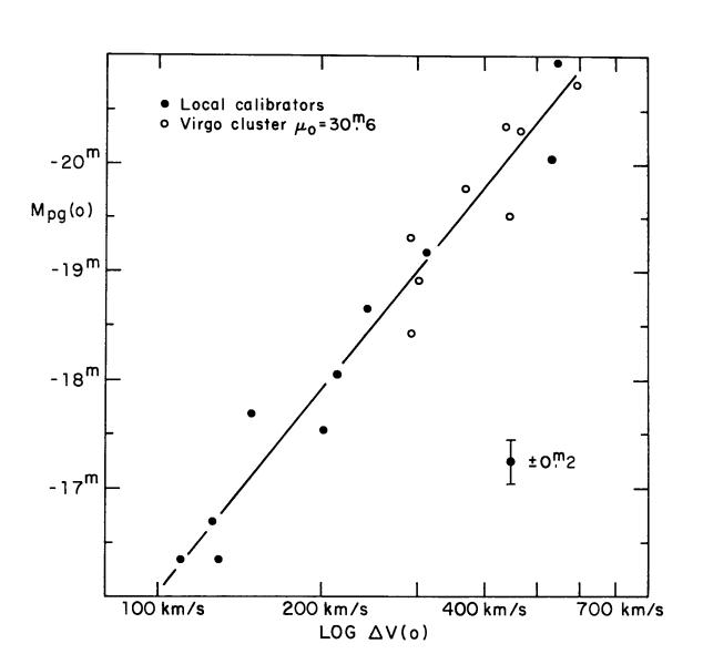
absolute brightness
log rotational velocity
Astronomy and Astrophysics, 54, 661
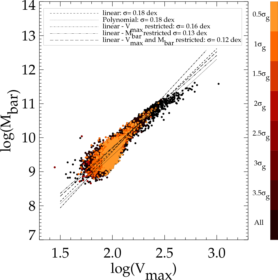
Astrophysics
The Tully–Fisher relation is an empirical relationship between the intrinsic luminosity of a spiral galaxy and its torational velocity
R. Brent Tully and J. Richard Fisher, 1977
log Mass
log rotational velocity
GRAVITY
Biology
Basal metabolism of mammals (that is, the minimum rate of energy generation of an organism) has long been known to scale empirically as
KLEIBER, M. (1932). Body size and metabolism. Hilgardia 6, 315
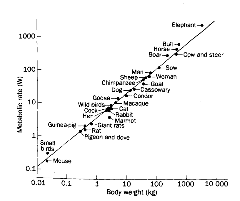
log metabolic rate
log weight
Biology
A general model that describes how essential materials are transported through space-filling fractal networks of branching tubes.
West, Brown, Enquist. 1997 Science
networks
G. West
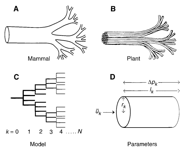
Diagrammatic examples of segments of biological distribution networks
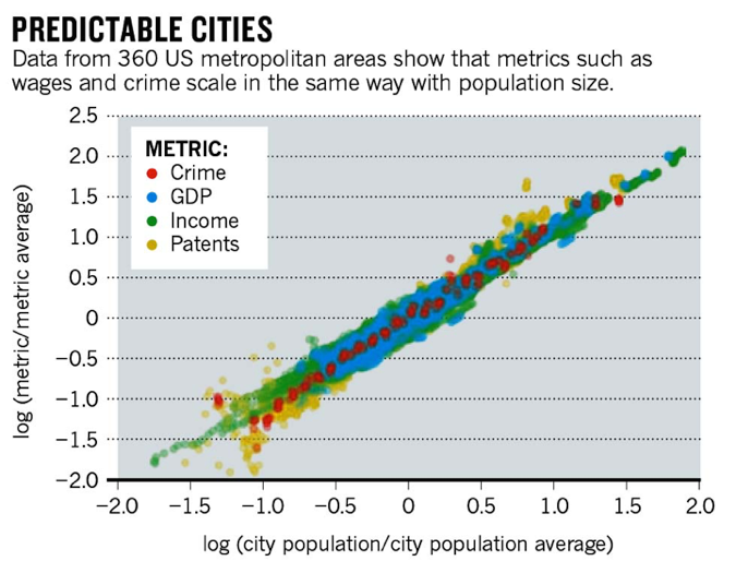
Urban Science
Cities are networks too! And they obey scaling laws on a ridiculus number of parameters!
Bettencourt, L. M. A., Lobo, J., Helbing, D., Kühnert, C. & West, G. B. Proc. Natl Acad. Sci. USA 104, 7301–7306 (2007)

G. West
key concepts
descriptive statistics
null hypothesis rejection testing setup
pivotal quantities
Z, t, χ2, K-S tests
the importance of scaling laws
homework
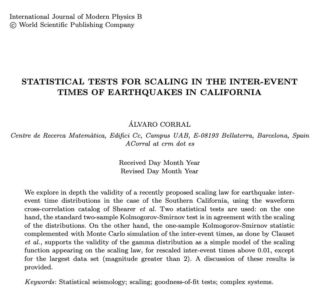
HW1 : earthquakes and KS test:
reproduce the work of Carrell 2018 using a KS-test to demonstrate the existence of s scaling law in the frequency of earthquakes
reading
watching
resources
Sarah Boslaugh, Dr. Paul Andrew Watters, 2008
Statistics in a Nutshell (Chapters 3,4,5)
https://books.google.com/books/about/Statistics_in_a_Nutshell.html?id=ZnhgO65Pyl4C
David M. Lane et al.
Introduction to Statistics (XVIII)
Bernard J. T. Jones, Vicent J. Martínez, Enn Saar, and Virginia Trimble
Scaling laws in physics
Bettencourt , Strumsky, West
Urban Scaling and Its Deviations: Revealing the Structure of Wealth, Innovation and Crime across Cities