


federica bianco
astro | data science | data for good
dr.federica bianco | fbb.space | fedhere | fedhere
Neural Networks: CNNs+autoencoders
this slide deck:
NN are a vast topics and we only have 2 weeks!
Some FREE references!
michael nielsen
better pedagogical approach, more basic, more clear
ian goodfellow
mathematical approach, more advanced, unfinished
michael nielsen
better pedagogical approach, more basic, more clear
0
Data driven models for exploration of structure, prediction that learn parameters from data.
Machine Learning
Data driven models for exploration of structure, prediction that learn parameters from data.
unupervised ------ supervised
set up: All features known for all observations
Goal: explore structure in the data
- data compression
- understanding structure
Algorithms: Clustering, (...)
x
y
Machine Learning
Data driven models for exploration of structure, prediction that learn parameters from data.
unupervised ------ supervised
set up: All features known for a sunbset of the data; one feature cannot be observed for the rest of the data
Goal: predicting missing feature
- classification
- regression
Algorithms: regression, SVM, tree methods, k-nearest neighbors, neural networks, (...)
x
y
Machine Learning
unupervised ------ supervised
set up: All features known for a sunbset of the data; one feature cannot be observed for the rest of the data
Goal: predicting missing feature
- classification
- regression
Algorithms: regression, SVM, tree methods, k-nearest neighbors, neural networks, (...)
unupervised ------ supervised
set up: All features known for all observations
Goal: explore structure in the data
- data compression
- understanding structure
Algorithms: k-means clustering, agglomerative clustering, density based clustering, (...)
Machine Learning
model parameters are learned by calculating a loss function for diferent parameter sets and trying to minimize loss (or a target function and trying to maximize)
e.g.
L1 = |target - prediction|
Learning relies on the definition of a loss function
Machine Learning
Learning relies on the definition of a loss function
| learning type | loss / target |
|---|---|
| unsupervised | intra-cluster variance / inter cluster distance |
| supervised | distance between prediction and truth |
Machine Learning
The definition of a loss function requires the definition of distance or similarity
Machine Learning
Minkowski distance
Jaccard similarity
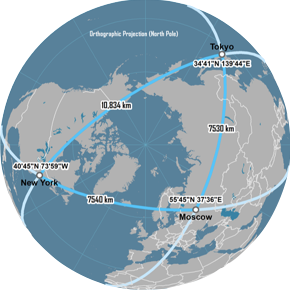
Great circle distance
The definition of a loss function requires the definition of distance or similarity
Machine Learning
Neural Networks
1
output
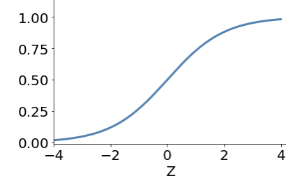
sigmoid
.
.
.
Perceptrons are linear classifiers:
makes predictions based on a linear predictor function
combining a set of weights (=parameters) with the feature vector.
weights
bias
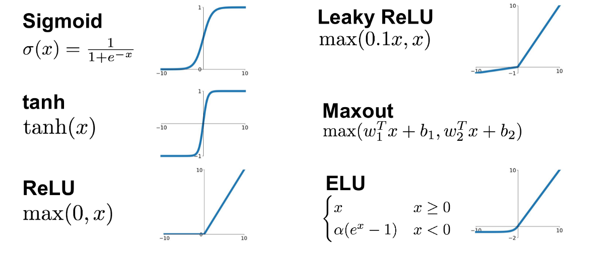
activation function
Turn a linear prediction into a binary or probabilistic classification
activation function
x1
x2
b1
b2
b3
b
w11
w12
w13
w21
w22
w23
w: weight
sets the sensitivity of a neuron
b: bias:
up-down weights a neuron
yes/no
x1
x2
b1
b2
b3
b
w11
w12
w13
w21
w22
w23
w: weight
sets the sensitivity of a neuron
b: bias:
up-down weights a neuron
yes/no
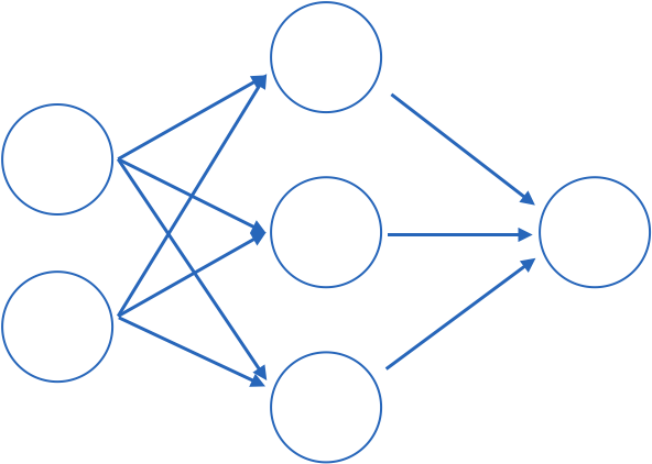
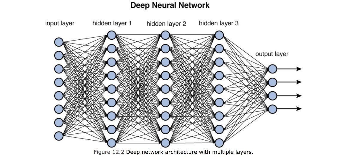
connected: all nodes go to all nodes of the next layer.
activation function
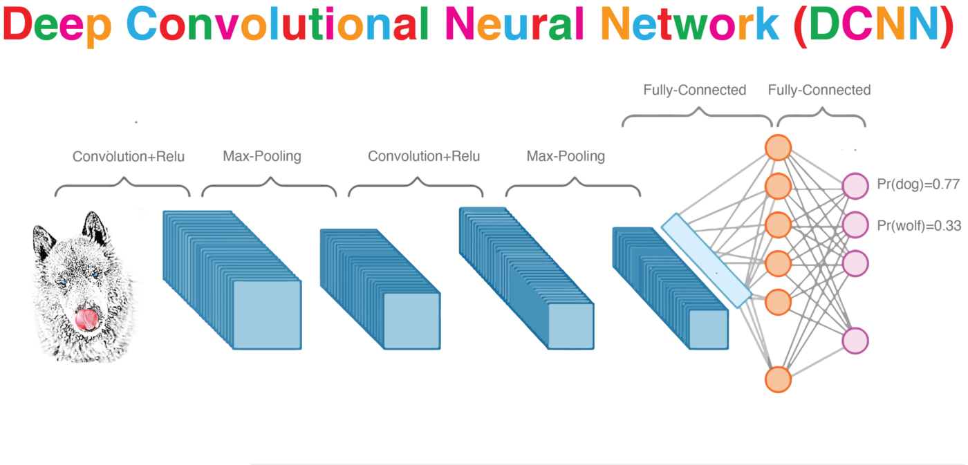
Deep Neural Networks
2
output
input layer
hidden layer
output layer
Fully connected: all nodes go to all nodes of the next layer.
output
input layer
hidden layer
output layer
Sparcely connected: all nodes go to all nodes of the next layer.
output
input layer
hidden layer
output layer
Sparcely connected: all nodes go to all nodes of the next layer.
The last layer is always connected
1x3
3x5
5x2
=
2x1
what we are doing is just a series of matrix multiplictions.
what we are doing is exactly a series of matrix multiplictions.
3x5
5x2
2x1
=
what we are doing is exactly a series of matrix multiplictions.
3x5
5x2
2x1
=
what we are doing is exactly a series of matrix multiplictions.
3x5
5x2
2x1
=
what we are doing is exactly a series of matrix multiplictions.
3x5
5x2
2x1
=
what we are doing is exactly a series of matrix multiplictions.
The purpose is to approximate a function φ
y = φ(x)
which (in general) is not linear with linear operations
The purpose is to approximate a function φ
y = φ(x)
which (in general) is not linear with linear operations
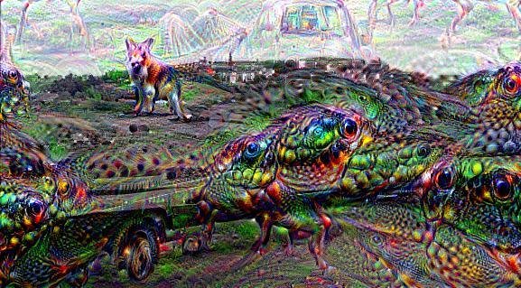
@akumadog
@akumadog
@akumadog
@akumadog
@akumadog
@akumadog
@akumadog
@akumadog
@akumadog
@akumadog
@akumadog
@akumadog
@akumadog
@akumadog
@akumadog
@akumadog
@akumadog
@akumadog
@akumadog
@akumadog
@akumadog
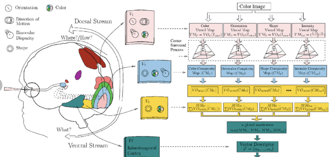
The visual cortex learns hierarchically: first detects simple features, then more complex features and ensembles of features
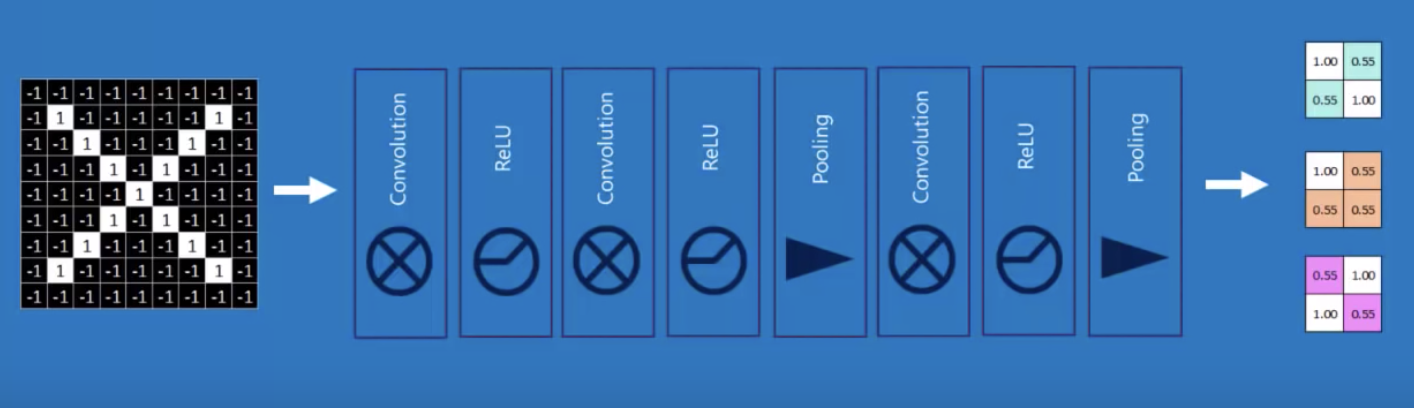
Convolution
convolution is a mathematical operator on two functions
f and g
that produces a third function
f x g
expressing how the shape of one is modified by the other.
o
two images.
| -1 | -1 | -1 | -1 | -1 |
|---|---|---|---|---|
| -1 | -1 | -1 | ||
| -1 | -1 | -1 | -1 | |
| -1 | -1 | -1 | ||
| -1 | -1 | -1 | -1 | -1 |
1
1
1
1
1
1
1
1
1
| -1 | -1 | -1 | -1 | -1 |
|---|---|---|---|---|
| -1 | -1 | -1 | -1 | -1 |
| -1 | -1 | -1 | -1 | -1 |
| -1 | -1 | -1 | -1 | -1 |
| -1 | -1 | -1 | -1 | -1 |
| 1 | -1 | -1 |
| -1 | 1 | -1 |
| -1 | -1 | 1 |
1
1
1
1
1
| -1 | -1 | -1 | -1 | -1 |
|---|---|---|---|---|
| -1 | -1 | -1 | ||
| -1 | -1 | -1 | -1 | |
| -1 | -1 | -1 | ||
| -1 | -1 | -1 | -1 | -1 |
| -1 | -1 | 1 |
| -1 | 1 | -1 |
| 1 | -1 | -1 |
feature maps
1
1
1
1
1
convolution
| -1 | -1 | -1 | -1 | -1 |
|---|---|---|---|---|
| -1 | -1 | -1 | ||
| -1 | -1 | -1 | -1 | |
| -1 | -1 | -1 | ||
| -1 | -1 | -1 | -1 | -1 |
| 1 | -1 | -1 |
| -1 | 1 | -1 |
| -1 | -1 | 1 |
1
1
1
1
1
| -1 | -1 | -1 | -1 | -1 |
|---|---|---|---|---|
| -1 | -1 | -1 | ||
| -1 | -1 | -1 | -1 | |
| -1 | -1 | -1 | ||
| -1 | -1 | -1 | -1 | -1 |
| 1 | -1 | -1 |
| -1 | 1 | -1 |
| -1 | -1 | 1 |
| 1 | -1 | -1 |
| -1 | 1 | -1 |
| -1 | -1 | 1 |
| 7 | ||
|---|---|---|
=
1
1
1
1
1
| -1 | -1 | -1 | -1 | -1 |
|---|---|---|---|---|
| -1 | -1 | -1 | ||
| -1 | -1 | -1 | -1 | |
| -1 | -1 | -1 | ||
| -1 | -1 | -1 | -1 | -1 |
| 1 | -1 | -1 |
| -1 | 1 | -1 |
| -1 | -1 | 1 |
| 1 | -1 | -1 |
| -1 | 1 | -1 |
| -1 | -1 | 1 |
| 7 | -3 | |
|---|---|---|
=
1
1
1
1
1
| -1 | -1 | -1 | -1 | -1 |
|---|---|---|---|---|
| -1 | -1 | -1 | ||
| -1 | -1 | -1 | -1 | |
| -1 | -1 | -1 | ||
| -1 | -1 | -1 | -1 | -1 |
| 1 | -1 | -1 |
| -1 | 1 | -1 |
| -1 | -1 | 1 |
| 1 | -1 | -1 |
| -1 | 1 | -1 |
| -1 | -1 | 1 |
| 7 | -3 | 3 |
|---|---|---|
=
1
1
1
1
1
| -1 | -1 | -1 | -1 | -1 |
|---|---|---|---|---|
| -1 | -1 | -1 | ||
| -1 | -1 | -1 | -1 | |
| -1 | -1 | -1 | ||
| -1 | -1 | -1 | -1 | -1 |
| 1 | -1 | -1 |
| -1 | 1 | -1 |
| -1 | -1 | 1 |
| 1 | -1 | -1 |
| -1 | 1 | -1 |
| -1 | -1 | 1 |
| 7 | -1 | 3 |
|---|---|---|
| ? | ||
=
1
1
1
1
1
| -1 | -1 | -1 | -1 | -1 |
|---|---|---|---|---|
| -1 | -1 | -1 | ||
| -1 | -1 | -1 | -1 | |
| -1 | -1 | -1 | ||
| -1 | -1 | -1 | -1 | -1 |
| 1 | -1 | -1 |
| -1 | 1 | -1 |
| -1 | -1 | 1 |
| 1 | -1 | -1 |
| -1 | 1 | -1 |
| -1 | -1 | 1 |
| 7 | -1 | 3 |
|---|---|---|
| ? | ? | |
=
1
1
1
1
1
| -1 | -1 | -1 | -1 | -1 |
|---|---|---|---|---|
| -1 | -1 | -1 | ||
| -1 | -1 | -1 | -1 | |
| -1 | -1 | -1 | ||
| -1 | -1 | -1 | -1 | -1 |
| 1 | -1 | -1 |
| -1 | 1 | -1 |
| -1 | -1 | 1 |
| 1 | -1 | -1 |
| -1 | 1 | -1 |
| -1 | -1 | 1 |
| 7 | -1 | 3 |
|---|---|---|
| ? | ? | |
=
1
1
1
1
1
| -1 | -1 | -1 | -1 | -1 |
|---|---|---|---|---|
| -1 | -1 | -1 | ||
| -1 | -1 | -1 | -1 | |
| -1 | -1 | -1 | ||
| -1 | -1 | -1 | -1 | -1 |
| 1 | -1 | -1 |
| -1 | 1 | -1 |
| -1 | -1 | 1 |
| 7 | -3 | 3 |
| -3 | 5 | -3 |
| 3 | -1 | 7 |
=
input layer
feature map
convolution layer
the feature map is "richer": we went from binary to R
1
1
1
1
1
| -1 | -1 | -1 | -1 | -1 |
|---|---|---|---|---|
| -1 | -1 | -1 | ||
| -1 | -1 | -1 | -1 | |
| -1 | -1 | -1 | ||
| -1 | -1 | -1 | -1 | -1 |
| 1 | -1 | -1 |
| -1 | 1 | -1 |
| -1 | -1 | 1 |
| 7 | -3 | 3 |
| -3 | 5 | -3 |
| 3 | -1 | 7 |
=
input layer
feature map
convolution layer
the feature map is "richer": we went from binary to R
and it is reminiscent of the original layer
7
5
7
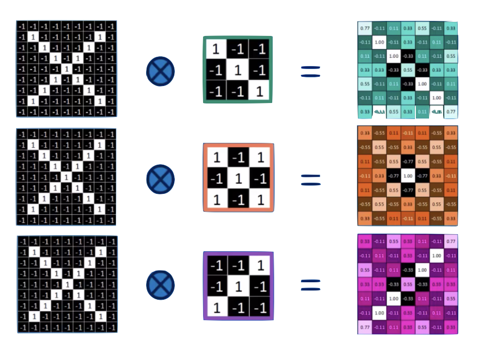
Convolve with different feature: each neuron is 1 feature
| 7 | -3 | 3 |
| -3 | 5 | -3 |
| 3 | -1 | 7 |
7
5
7
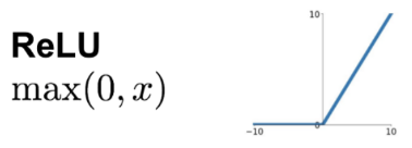
ReLu: normalization that replaces negative values with 0's
| 7 | 0 | 3 |
| 0 | 5 | 0 |
| 3 | 0 | 7 |
7
5
7
Max-Pool
MaxPooling: reduce image size, generalizes result
| 7 | 0 | 3 |
| 0 | 5 | 0 |
| 0 | 0 | 7 |
7
5
7
MaxPooling: reduce image size, generalizes result
| 7 | 0 | 3 |
| 0 | 5 | 0 |
| 3 | 0 | 7 |
7
5
7
2x2 Max Poll
| 7 | 5 |
MaxPooling: reduce image size, generalizes result
| 7 | 0 | 3 |
| 0 | 5 | 0 |
| 3 | 0 | 7 |
7
5
7
2x2 Max Poll
| 7 | 5 |
| 5 |
MaxPooling: reduce image size, generalizes result
| 7 | 0 | 3 |
| 0 | 5 | 0 |
| 3 | 0 | 7 |
7
5
7
2x2 Max Poll
| 7 | 5 |
| 5 | 7 |
MaxPooling: reduce image size & generalizes result
By reducing the size and picking the maximum of a sub-region we make the network less sensitive to specific details
training DNN
3
.
.
.
Any linear model:
y : prediction
ytrue : target
Error: e.g.
intercept
slope
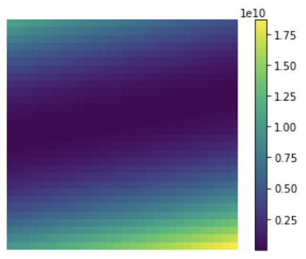
L2
x
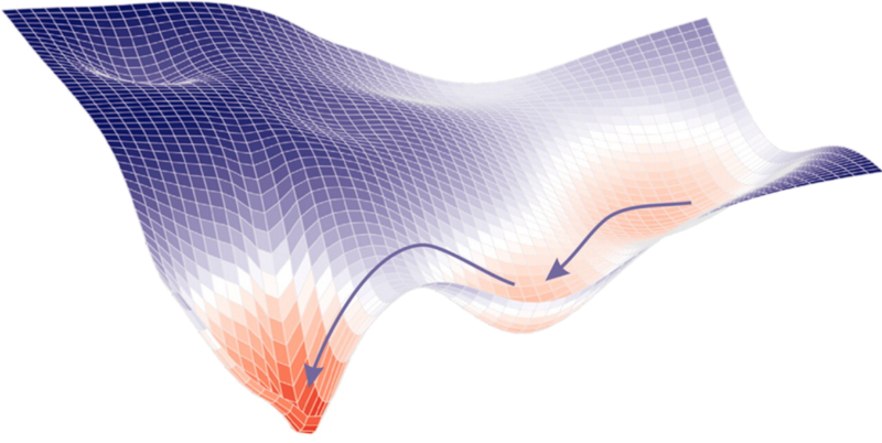
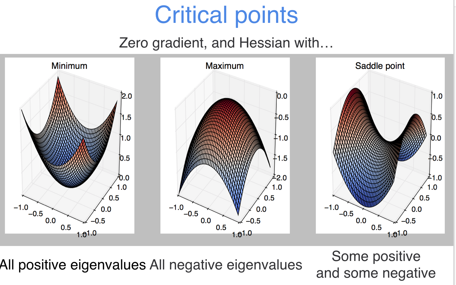
Find the best parameters by finding the minimum of the L2 hyperplane
at every step look around and choose the best direction
.
.
.
Any linear model:
y : prediction
ytrue : target
Error: e.g.
intercept
slope
L2
Find the best parameters by finding the minimum of the L2 hyperplane
at every step look around and choose the best direction
at every step look around and choose the best direction
Training models with this many parameters requires a lot of care:
. defining the metric
. optimization schemes
. training/validation/testing sets
But just like our simple linear regression case, the fact that small changes in the parameters leads to small changes in the output for the right activation functions.
define a cost function, e.g.
Training a feed-forward DNN
feed data forward through network and calculate cost metric
for each layer, calculate effect of small changes on next layer
Training models with this many parameters requires a lot of care:
. defining the metric
. optimization schemes
. training/validation/testing sets
earlier layers learn more slowly
Training a feed-forward DNN
Loss functions: with NN you often encounter this loss function
negative loglikelihood or cross entropy
if
how does linear descent look when you have a whole network structure with hundreds of weights and biases to optimize??
.
.
.
output
Training a feed-forward DNN
how does linear descent look when you have a whole network structure with hundreds of weights and biases to optimize??
Training a feed-forward DNN
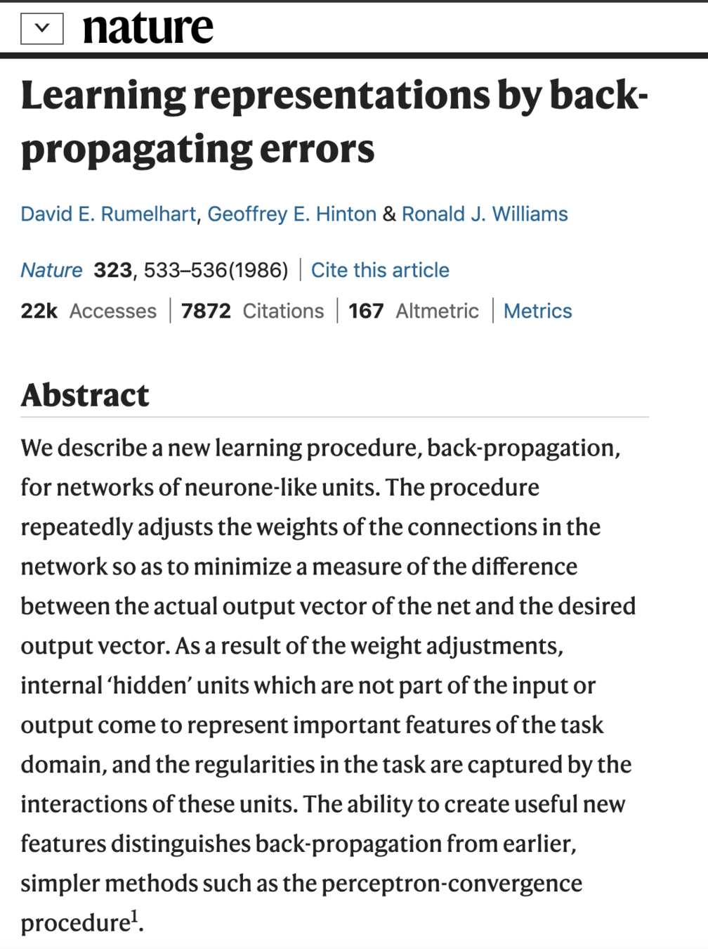
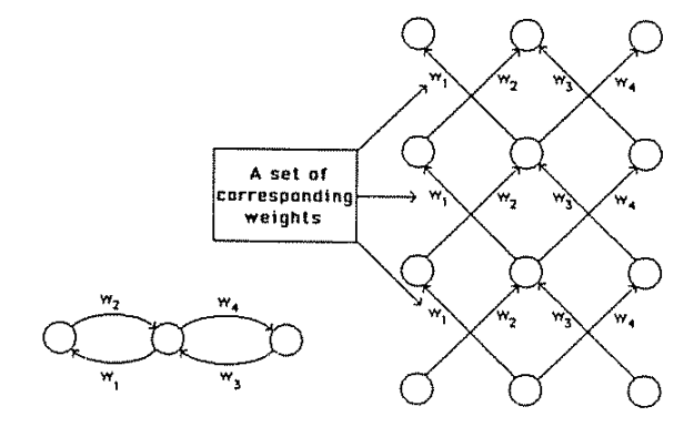
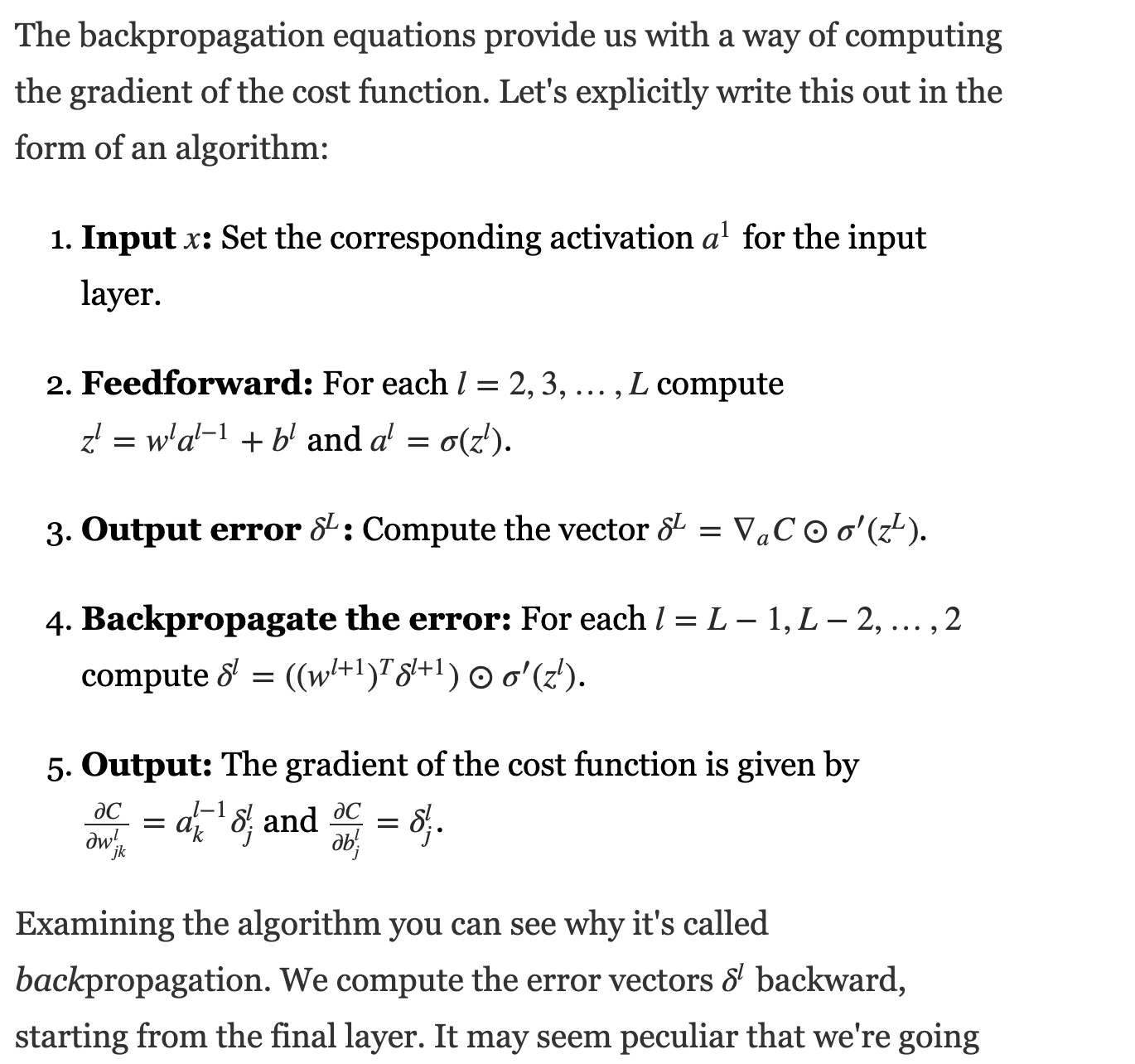
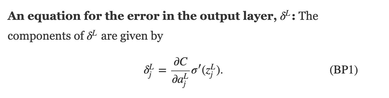
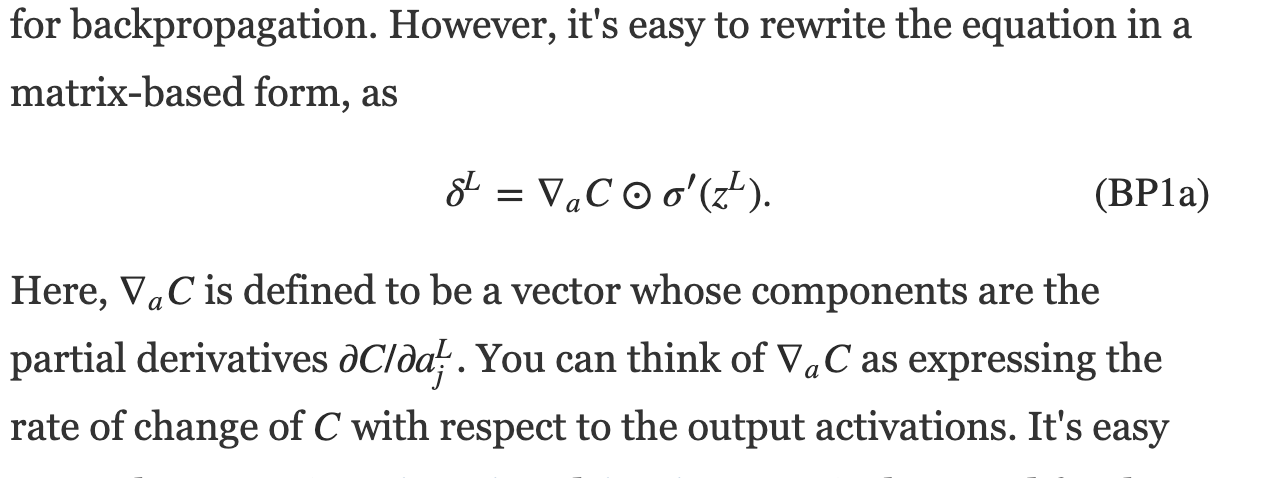
- we want to get the gradient to use it in downhill optimization
backprop is a dynamic programming algorithm that calculates all gradients than looks them up
Training a feed-forward DNN
- we want to get the gradient to use it in downhill optimization
- chain rule
Training a feed-forward DNN
This is the simplest deep NN: one neuron per layer
these are the changes on the last layer w respect to w and b
Training a feed-forward DNN
Training a feed-forward DNN
This is the simplest deep NN: one neuron per layer
x
z1
z2
z3
z4
how does linear descent look when you have a whole network structure with hundreds of weights and biases to optimize??
think of applying just gradient to a function of a function of a function... use:
1) partial derivatives, 2) chain rule
define a cost function, e.g.
Training a DNN
Training a DNN
build a DNN from scratch using numpy
Autoencoders
4
Unsupervised learning with
Neural Networks
What do NN do? approximate complex functions with series of linear functions
.... so if my layers are smaller what I have is a compact representation of the data
}
5dim representation
4dim
3dim
complex imput data
Unsupervised learning with
Neural Networks
What do NN do? approximate complex functions with series of linear functions
To do that they extract information from the data
Each layer of the DNN produces a representation of the data a "latent representation" .
The dimensionality of that latent representation is determined by the size of the layer (and its connectivity, but we will ignore this bit for now)
.... so if my layers are smaller what I have is a compact representation of the data
}
5dim representation
4dim
3dim
complex imput data
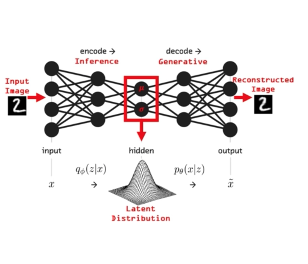
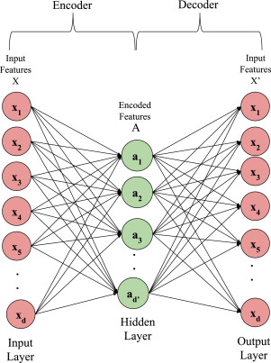
Autoencoder Architecture
Feed Forward DNN:
the size of the input is 5,
the size of the last layer is 2
Autoencoder Architecture
replicat the same structure backwards
Autoencoder Architecture
input
output
ask it to reproduce the input
if you have not lost informatoin in the compression you can reproduce the input closely!
the target of the Autoencoder is the data itself
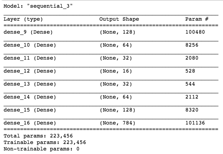
Autoencoder Architecture
Autoencoder Architecture
from keras.layers import Dense, Flatten, Reshape, Input, InputLayer
from keras.models import Sequential, Model

def build_autoencoder(image_shape, bn_size):
    # Encoder
    encoder = Sequential()
    encoder.add(InputLayer(img_shape))
    encoder.add(Flatten())
    encoder.add(Dense(bn_size))

    # Decoder
    decoder = Sequential()
    decoder.add(InputLayer((bn_size,)))
    decoder.add(Dense(np.prod(image_shape)))
    decoder.add(Reshape(image_shape))

    return encoder, decoder
Autoencoder Architecture
Building a DNN
with keras and tensorflow
Trivial to build, but the devil is in the details!
Building a DNN
with keras and tensorflow
Trivial to build, but the devil is in the details!
from keras.models import Sequential
#can upload pretrained models from keras.models
from keras.layers import Dense, Conv2D, MaxPooling2D
#create model
model = Sequential()
#create the model architecture by adding model layers
model.add(Dense(10, activation='relu', input_shape=(n_cols,)))
model.add(Dense(10, activation='relu'))
model.add(Dense(1))
#need to choose the loss function, metric, optimization scheme
model.compile(optimizer='adam', loss='mean_squared_error')
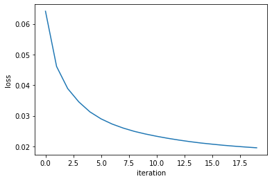
#need to learn what to look for - always plot the loss function!
model.fit(x_train, y_train, validation_data=(x_test, y_test),
epochs=20, batch_size=100, verbose=1)
#note that the model allows to give a validation test,
#this is for a 3fold cross valiation: train-validate-test
#predict
test_y_predictions = model.predict(validate_X)Building a DNN
with keras and tensorflow
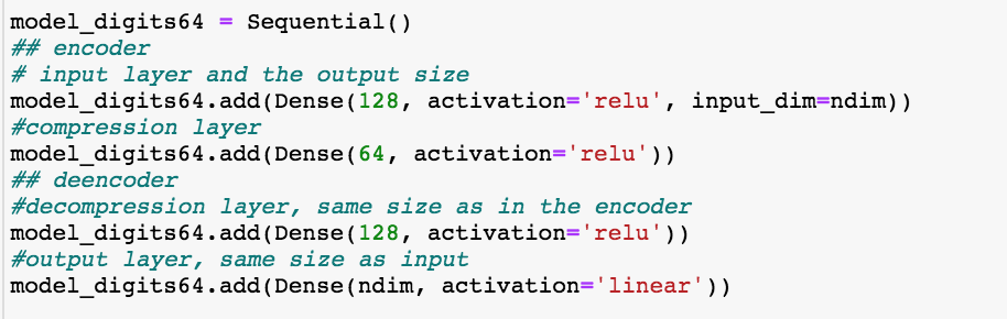
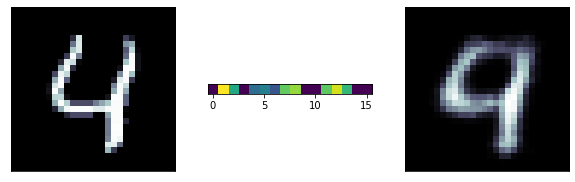
autoencoder for image recontstruction
encoder
This autoencoder model has a 64-neuron bottle neck. This means it will generate a compressed representation of the data out of that layer which is 16-dimensional (the original size is 784 pixels)
Building a DNN
with keras and tensorflow
autoencoder for image recontstruction
This autoencoder model has a 64-neuron bottle neck. This means it will generate a compressed representation of the data out of that layer which is 16-dimensional (the original size is 784 pixels)
Building a DNN
with keras and tensorflow
autoencoder for image recontstruction
decoder
This autoencoder model has a 64-neuron bottle neck. This means it will generate a compressed representation of the data out of that layer which is 16-dimensional (the original size is 784 pixels)
Building a DNN
with keras and tensorflow
autoencoder for image recontstruction
This autoencoder model has a 64-neuron bottle neck. This means it will generate a compressed representation of the data out of that layer which is 16-dimensional (the original size is 784 pixels)
bottle neck
Building a DNN
with keras and tensorflow
autoencoder for image recontstruction
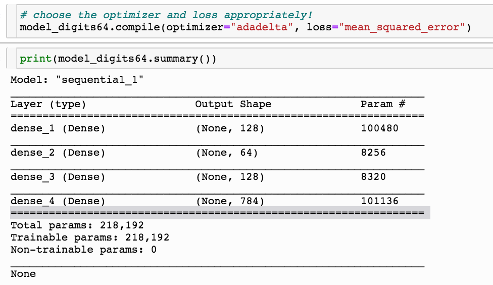
This simple odel has 200000 parameters!
My original choice is to train it with "adadelta" with a mean squared loss function, all activation functions are relu, appropriate for a linear regression
Building a DNN
with keras and tensorflow
autoencoder for image recontstruction
What should I choose for the loss function and how does that relate to the activation functiom and optimization?
Building a DNN
with keras and tensorflow
autoencoder for image recontstruction
What should I choose for the loss function and how does that relate to the activation functiom and optimization?
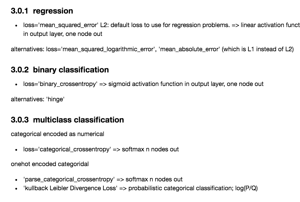
| loss | good for | activation last layer | size last layer |
|---|---|---|---|
| mean_squared_error | regression | linear | one node |
| mean_absolute_error | regression | linear | one node |
| mean_squared_logarithmit_error | regression | linear | one node |
| binary_crossentropy | binary classification | sigmoid | one node |
| categorical_crossentropy | multiclass classification | sigmoid | N nodes |
| Kullback_Divergence | multiclass classification, probabilistic inerpretation | sigmoid | N nodes |
autoencoder for image recontstruction
model_digits64.add(Dense(ndim,
                        activation='linear'))
model_digits64_sig.compile(optimizer="adadelta",
                   loss="mean_squared_error")
model_digits64_sig.add(Dense(ndim,
activation='sigmoid'))
model_digits64_sig.compile(optimizer="adadelta",
loss="mean_squared_error")
model_digits64_sig.add(Dense(ndim,
activation='sigmoid'))
model_digits64_bce.compile(optimizer="adadelta",
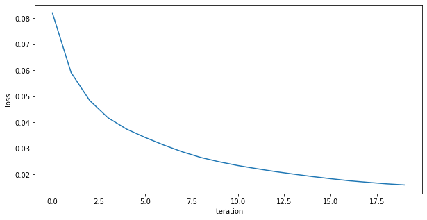
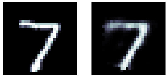
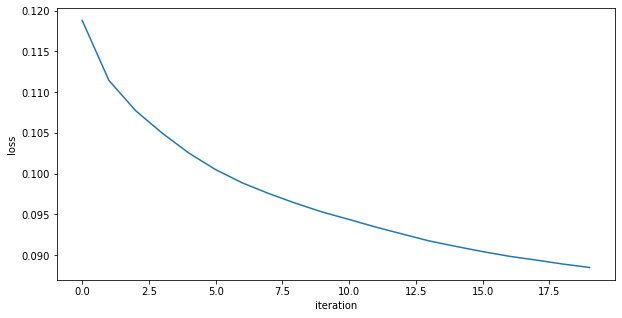
loss="binary_crossentropy")loss function: did not finish learning, it is still decreasing rapidly
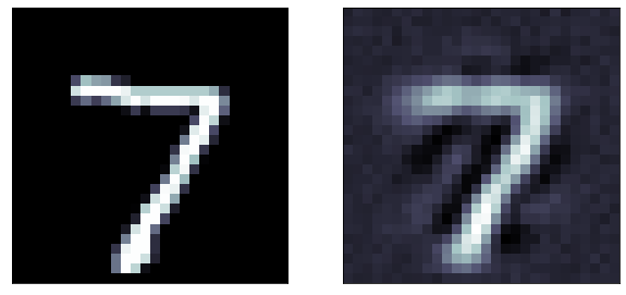
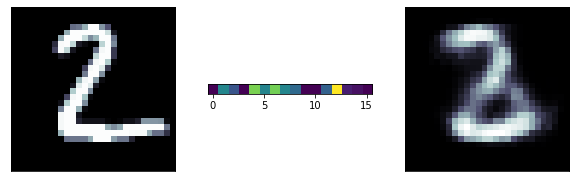
The predictions are far too detailed. While the input is not binary, it does not have a lot of details. Maybe approaching it as a binary problem (with a sigmoid and a binary cross entropy loss) will give better results
loss function: also did not finish learning, it is still decreasing rapidly
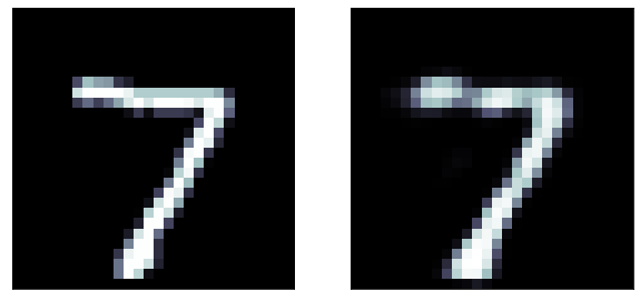
A sigmoid gives activation gives a much better result!
Binary cross entropy loss function: It is more appriopriate when the output layer is sigmoid
Even better results!
original
predicted
predicted
original
predicted
original
predicted
autoencoder for image recontstruction
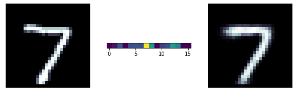
A more ambitious model has a 16 neurons bottle neck: we are trying to extract 16 numbers to reconstruct the entire image! its pretty remarcable! those 16 number are extracted features from the data
predicted
original
latent
representation
autoencoder for image recontstruction
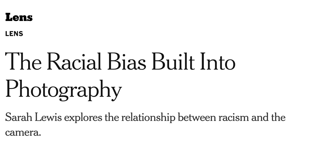
The bias is in the data
The bias is in the models and the decision we make
The bias is in how we choose to optimize our model
Should AI reflect
who we are
(and enforce and grow our bias)
or should it reflect who we aspire to be?
(and who decides what that is?)
The bias is society that provides the framework to validate our biased models
The bias is in the data
The bias is in the models and the decision we make
The bias is in how we choose to optimize our model
The bias is society that provides the framework to validate our biased models
none of this is new
https://www.nytimes.com/2019/04/25/lens/sarah-lewis-racial-bias-photography.html
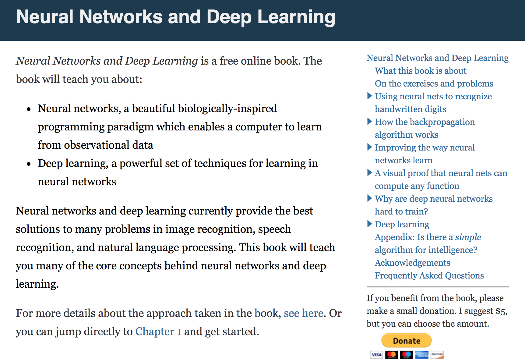
Neural Network and Deep Learning
an excellent and free book on NN and DL
http://neuralnetworksanddeeplearning.com/index.html
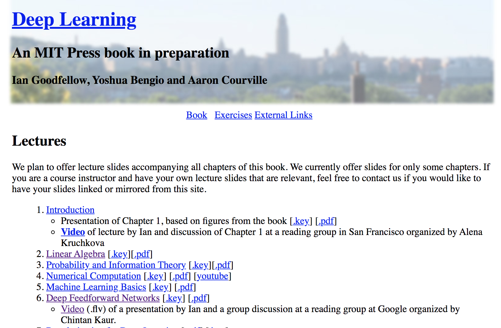
Deep Learning An MIT Press book in preparation
Ian Goodfellow, Yoshua Bengio and Aaron Courville
https://www.deeplearningbook.org/lecture_slides.html
History of NN
https://cs.stanford.edu/people/eroberts/courses/soco/projects/neural-networks/History/history2.html
By federica bianco
Autoencoders


