


federica bianco
astro | data science | data for good
dr.federica bianco | fbb.space | fedhere | fedhere
NHRT
1. overfitting
2. p-value inference
3. mapping in python (intro to geopandas)
descriptive statistics
1
are these 2 numbers the same?
clearly 1.2 = 1.8
are these 2 numbers the same?
two numbers are never actually the same, but we understand that there are limitations in how well numbers represent reality
1.2+/- 1 = 1.8+/- 1
because the [0.2-2.2] interval overlaps the [0.8-2.8] interval
All data has some element of randomness either because:
All data has some element of randomness either because:
we think of data points as a number extracted from a distribution. sometimes we have expectations for that distribution, sometimes we do not.
observational approach: a distribution represent the frequency with which we obtain a value ~x when measuring a phenomenon
number of values
measured between
x and x+dx
x
analyst approach: a distribution represent the probability with which a phenomenon generates a value that we measure to be ~x
frequency
probability
normal or Gaussian
continuous support
Poisson
discrete support
fraction of draws
fraction of draws
normal or Gaussian
continuous support
Poisson
discrete support
parameters (lambda=10)
parameters
support
fraction of draws
fraction of draws
parameters (-0.1, 0.9)
support
normal or Gaussian
continuous support
Poisson
discrete support
parameters (lambda=1)
means: 1, 2
standard deviation: 1, 1
are these distributions the same?
a distribution’s moments summarize its properties:
central tendency: mean (n=1), median, mode (peak)
spread: standard deviation/variance (n=2), quartiles
symmetry: skewness (n=3)
cuspiness: kurtosis (n=4)
Normal
Chi-squared
a distribution’s moments summarize its properties:
central tendency: mean (n=1), median, mode (peak)
spread: standard deviation (variance n=2), quartiles
symmetry: skewness (n=3)
cuspiness: kurtosis (n=4)
a distribution’s moments summarize its properties:
central tendency: mean (n=1), median, mode (peak)
spread: standard deviation (variance n=2), quartiles
symmetry: skewness (n=3)
cuspiness: kurtosis (n=4)
a distribution’s moments summarize its properties:
central tendency: mean (n=1), median, mode (peak)
spread: standard deviation (variance n=2), quartiles
symmetry: skewness (n=3)
cuspiness: kurtosis (n=4)
are these distributions the same?
if distributions have the same measured means within 1 (or n) standard deviation they should be considered "the same"
means: 1,2
standard deviation: 1,1
1.5*IQR
IQR interquartile range (25%-75%)
mean
a distribution’s moments summarize its properties:
central tendency: mean (n=1), median, mode (peak)
spread: standard deviation (variance n=2), quartiles
symmetry: skewness (n=3)
cuspiness: kurtosis (n=4)
p-value hypothesis testing
2
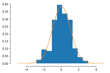
Imagine that I take a measurements of a quantity that is expected to be normally distributed with mean 0 and stdev 1
what is the probability that I would measure 1.5?
16%
16%
The probability of measuring any one value is mathematically 0... however I can say that
the probability of measuring something between -1σ and 1σ (within 1-sigma) is 68%.
So the probability of measuring something outside is 100-68 = 32%.
So if I measure something outside of [-1σ:1σ] that had a probability <32% of being measured.
Imagine that I take a measurements of a quantity that is expected to be normally distributed with mean 0 and stdev 1
what is the probability that I would measure 1.5?
The probability of measuring any one value is mathematically 0... however I can say that
the probability of measuring something between -2σ and 2σ (within 2-sigma) is 95%.
So the probability of measuring something outside is 100-95 = 5%.
So if I measure something outside of [-2σ:2σ] that had a probability <5% of being measured.
Imagine that I take a measurements of a quantity that is expected to be normally distributed with mean 0 and stdev 1
what is the probability that I would measure 1.5?
The probability of measuring any one value is mathematically 0... however I can say that
the probability of measuring something between -3σ and 3σ (within 3-sigma) is 99.7%.
So the probability of measuring something outside is 100-99.7 = 0.3%.
So if I measure something outside of [-3σ:3σ] that had a probability <0.3% of being measured.
Imagine that I take a measurements of a quantity that is expected to be normally distributed with mean 0 and stdev 1
what is the probability that I would measure 1.5?
it might be easier to think about it as cumulative distributions if you are comfortable with integrals
the probability of measuring something between -3σ and 3σ (within 3-sigma) is 99.7%.
So the probability of measuring something outside is 100-99.7 = 0.3%.
So if I measure something outside of [-3σ:3σ] that had a probability <0.3% of being measured.
Distribution of measurements under the Null hypothesie
2σ
Null hypothesis rejected
(p-value 0.05)
Null hypothesis cannot be rejected at a
p-value 0.05
set up threshold α
its important to do this first. If we do not we may be tempted to choose a threshold that fits our result, thus always reporting rejection of null hypothesis
set up threshold α
identify how you expect your measurement to be distributed under the Null hypothesis
set up threshold α
identify how you expect your measurement to be distributed under the Null hypothesis
measure outcome from data: x0
set up threshold α
identify how you expect your measurement to be distributed under the Null hypothesis
falsify H0
measure outcome from data: x0
H0 cannot be falsified
set up threshold α
identify how you expect your measurement to be distributed under the Null hypothesis
falsify H0
measure outcome from data: x0
H0 cannot be falsified
this quantity is called a "statistics"
statistics
2.1
In NHRT a statistics is a quantity that relates to the data which has a known distribution under the Null Hypothesis
e.g.: Z statistics is Normally distributed Z~N(0,1)
In absence of effect (i.e. under the Null)
== the sample mean is the same as the population mean
Z is distributed according to a Gaussian N(μ=0, σ=1)
Does a sample come from a known population? Z -test
Example: new bus route implementation.
https://github.com/fedhere/PUS2022_FBianco/blob/master/classdemo/ZtestBustime.ipynb
You know the mean and standard deviation of a but travel route: that is the population
You measure the new travel time between two stops 10 times: that is your sample.
Has travel time changed?
2σ
95%
In absence of effect (i.e. under the Null)
== the proportions of men and women are the same
Z is distributed according to a Gaussian N(μ=0, σ=1)
Are 2 proportions (fractions) the same? Z -test
Example: citibike women usage patterns
https://github.com/fedhere/PUS2020_FBianco/blob/master/classdemo/citibikes_gender.ipynb
You want to know if women are less likely than man to use citibike to commute.
You know the fraction of rides women (men) take during the week
2σ
95%
Are 2 proportions (fractions) the same? Z -test
Example: citibike women usage patterns
Citibikes is the bike share system in place in NYC
They have pioneered not only bikeshare but also open data on the bikes usage
e.g. https://www.kaggle.com/datasets/sujan97/citibike-system-data
https://github.com/fedhere/PUS2022_FBianco/blob/master/classdemo/citibikes_gender.ipynb
You want to know if customers identifying as women are less likely than customers identifying as men to use citibike to commute (commute as opposed to recreational use)
Commuting is more likely to happen during weekdays as most people have weekday jobs, than over the weekend, so
Assumption: weekday trips are commuting trips, weekend trips are recreational trips
You know the fraction of rides women (men) take during the week
Statistics and tests
data kinds and nomenclature
3
Types of Data:
Data Definitions
Data: observations that have been collected
Population: the complete body of subjects we want to infer about
Sample: the subset of the population about which data is collected/available
Census: collection of data from the entire population
Parameter: the subset of the population we actually studied collection of data from the entire population
Statistics: numerical value describing an attribute of the population numerical value describing an attribute of the sample
Data Definitions
The analysis of our ______
showed that for our 10 _________ the mean income is $60k. The standard deviation of the ______ means is $12k. From this _______ we infer for the _____________ a mean income _________ $60k +/- $12k
data
sample
statistics
population
parameter
At the root is the fact that a sample drawn from a parent distribution will look increasingly more like the parent distribution as the size of the sample increases.
More formally: The distribution of the means of N samples generated from the same parent distribution will
I. be normally distributed (i.e. will be a Gaussian)
II. have mean equal to the mean of the parent distribution, and
III. have standard deviation equal to the parent population standard deviation divided by the square root of the sample size
Qualitative variables
No ordering
UrbanScience e.g. precinct, state, gender, Also called Nominal, Categorical
Types of Data:
Qualitative variables
No ordering
UrbanScience e.g. precinct, state, gender, Also called Nominal, Categorical
Quantitative variables
Ordering is meaningful
Time, Distance, Age, Length, Intensity, Satisfaction, Number of
Types of Data:
Qualitative variables
No ordering
UrbanScience e.g. precinct, state, gender, Also called Nominal, Categorical
Quantitative variables
Ordering is meaningful
Time, Distance, Age, Length, Intensity, Satisfaction, Number of
Counts:
number of people in a county
Ordinal:
survey response Good/Fair/Poor
discrete
Types of Data:
Qualitative variables
No ordering
UrbanScience e.g. precinct, state, gender, Also called Nominal, Categorical
Quantitative variables
Ordering is meaningful
Time, Distance, Age, Length, Intensity, Satisfaction, Number of
continuous
Counts:
number of people in a county
Ordinal:
survey response Good/Fair/Poor
Continuous
Ordinal:
Earthquakes (notlinear scale)
Interval:
F temperature interval size preserved
Ratio:
Car speed
0 is naturally defined
discrete
Censored: age>90
Missing: “Prefer not to answer” (NA / NaN)
Types of Data:
which is the right test for me?
4
epistemological rooots of overfitting
4
Ockham’s razor: Pluralitas non est ponenda sine neccesitate
or “the law of parsimony”
William of Ockham (logician and Franciscan friar) 1300ca
but probably to be attributed to John Duns Scotus (1265–1308)
”Complexity needs not to be postulated without a need for it”
“Between 2 theories choose the simpler one”
“Between 2 theories choose the one with fewer parameters"
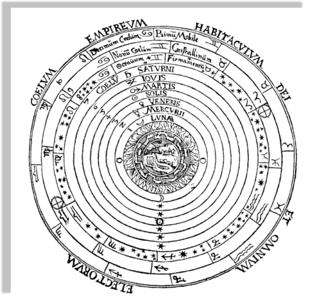
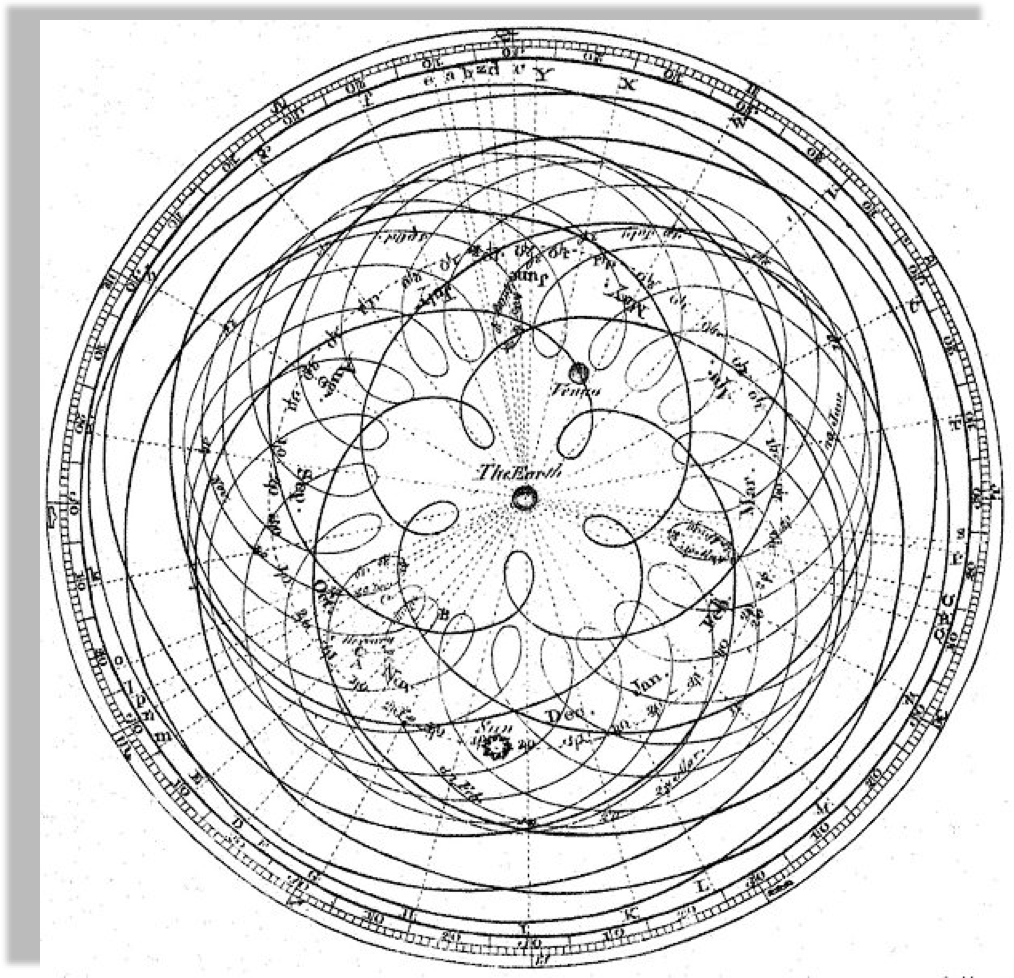
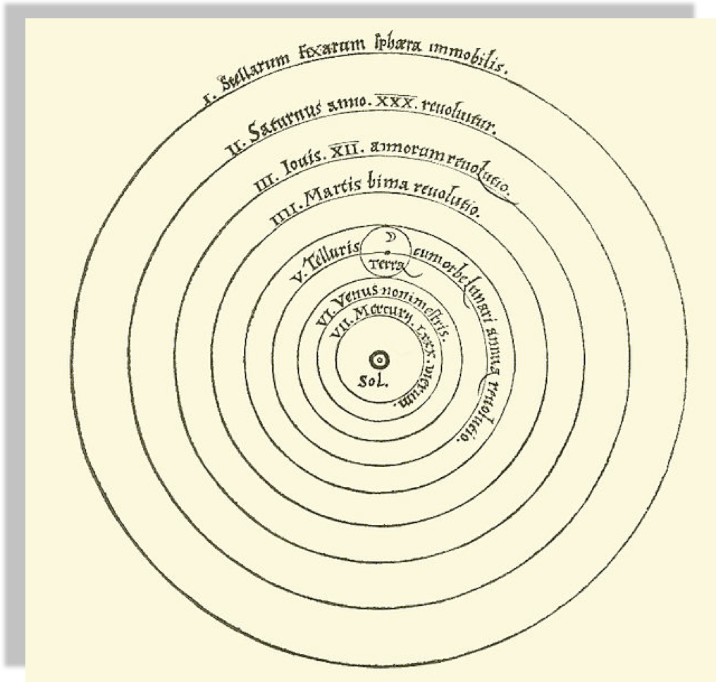
Heliocentric model from Nicolaus Copernicus'
"De revolutionibus orbium coelestium".
Author Dr Long's copy of Cassini, 1777
Peter Apian, Cosmographia, Antwerp, 1524
Heliocentric model from Nicolaus Copernicus'
"De revolutionibus orbium coelestium".
Author Dr Long's copy of Cassini, 1777
Two theories may explain a phenomenon just as well as each other. In that case you should prefer the simpler one
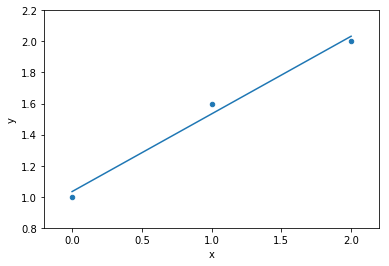
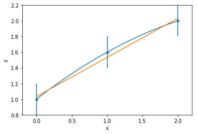
data
model fit to data
model fit to data
model fit to data
1 variable: x
model fit to data
parameters
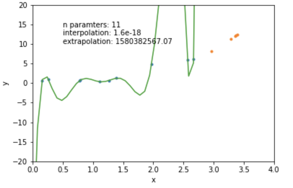
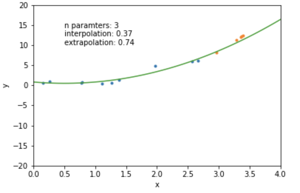
the complexity of a model can be measured by the number of variables and the numbers of parameters
the complexity of a model can be measured by the number of variables and the numbers of parameters
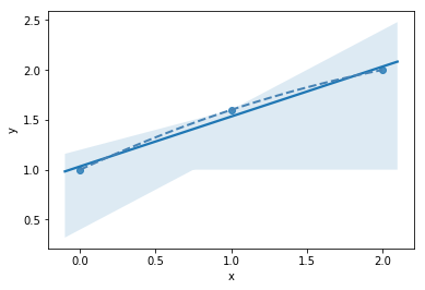
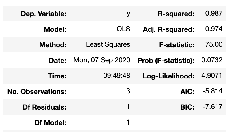
mathematically: given N data points there exist an N-features model that goes exactly through each data point. but is it useul??
Overfitting: fitting data with a model that is too complex and that does not extend to new data (low predictive power on test data)
data
model fit to data
Descriptive statistics: mean, median, standard deviation, interquartile range
Definition: Types of data
NHRT Null Hypothesis Rejection Testing and p-values
Definition: Parameters, features, variables
Statistical tests:
how to use it (statistics value compared to the distribution under the null)
how to choose it : what kind of data? what kind of question?
Distributions: frequency and probability interpretations
From idea to hypothesis
idea
measurable quantity
statistics
H0 Null hypothesis
Ha Alternative hypothesis
falsify H0
set up threshold α
identify how you expect your measurement to be distributed under the Null hypothesis
falsify H0
measure outcome from data: x0
H0 cannot be falsified
{
NHRT setup:
set up threshold α
identify how you expect your measurement to be distributed under the Null hypothesis
falsify H0
measure outcome from data: x0
H0 cannot be falsified
By federica bianco
p-value | reproducible mapping


