Field-level inference from galaxy surveys
Context

🫁
🚬
☢️
🚗
https://www.cancer-environnement.fr/fiches/cancers/cancer-du-poumon/
$$\mathbb O(🤒 \mid ➕) = \operatorname{BF}(➕)\; \mathbb O(🤒) = \frac{\mathbb P(🤒 \mid ➕)}{1-\mathbb P(🤒 \mid ➕)}$$
$$\begin{align*}\mathbb P(🤒 \mid ➕) &= \frac{\operatorname{BF}(➕) \;\mathbb O(🤒)}{1+\operatorname{BF}(➕) \; \mathbb O(🤒)} = \frac{\mathbb P(➕\mid🤒) \mathbb P(🤒)}{\mathbb P(➕\mid😊)\mathbb P(😊)+\mathbb P(➕\mid🤒) \mathbb P(🤒)}\\ &= \frac{\mathbb P(➕\mid🤒) }{\mathbb P(➕)}\mathbb P(🤒)\end{align*}$$
$$\operatorname{BF}(➕) := \frac{\mathbb P(➕\mid🤒)}{\mathbb P(➕\mid😊)}$$
$$\begin{align*}\mathbb P(🤒 \mid ➕) = \frac{\mathbb P(➕\mid🤒) }{\mathbb P(➕)}\mathbb P(🤒)\end{align*}$$
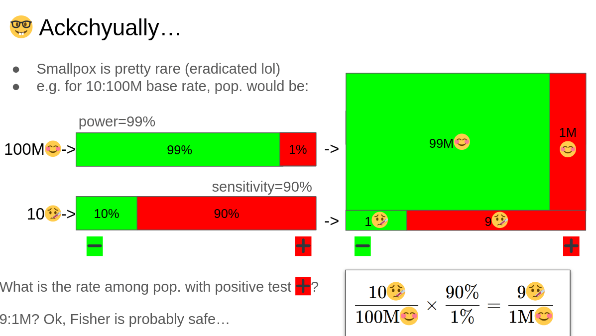
$$\frac{10🤒}{100\text{M}😊}\times \frac{90\%}{1\%}= \frac{9🤒}{1\text{M}😊}$$
$$\log \operatorname{BF}(D)=2.4$$
$$\log\mathbb O(\Lambda\text{CDM})$$
$$\log\mathbb O(w_0 w_a\text{CDM})$$
$$M$$
$$M\mid D$$
$$\frac{9🤒}{1\text{M}😊} = \frac{90\%}{1\%} \times \frac{10🤒}{100\text{M}😊}$$
Invert?
Animate to make it increase
and maybe better down instead?
- model: model is defined by its joint proba \(p(x, y)\)
- Bayes Theorem (proba formulation):$$\begin{gather*}p(x \mid y)p(y) = p(x, y) = p(y \mid x)p(x)\\\iff\\\underbrace{p(x \mid y)}_{\text{posterior}} = \frac{\overbrace{p(y \mid x)}^{\text{likelihood}}}{\underbrace{p(y)}_{\text{evidence}}}\underbrace{p(x)}_{\text{prior}}\end{gather*}$$
-
a priori meaning “from before (observation)”
-
a posteriori meaning “from after (observation)”
-
evidence/prior predictive: data evidence, how much the data is evident per se. Alias prior predictive, information on data a priori $$p(y) := \int p(y \mid x) p(x) \mathrm{d} x$$
-
posterior predictive: information on data a posteriori$$p(y_1 \mid y_0) := \int p(y_1 \mid x) p(x \mid y_0) \mathrm{d} x$$
-
Bayes factor/likelihood ratio: \(\operatorname{BF}(y \mid x_1, x_0):= \frac{p(y_0 \mid x_1)}{p(y_0 \mid x_0)}\)
- Inference meaning “to transport, propagate (information)”
- Bayes Theorem (information formulation):$$H(X \mid Y) = H(Y \mid X) - H(Y) + H(X)$$Moreover$$H(X) - H(X \mid Y) = H(X) + H(Y) - H(X, Y) = I(X;Y) \geq 0$$
$$\mathbb P(X > x \mid H_0)$$
$$\frac{\mathbb P(x\mid H_1)}{\mathbb P(x \mid H_0)}$$
\(\theta\mapsto\mathbb P(R(X) \ni \theta \mid \theta)\)
\(\mathbb P(\theta \in R(X) \mid X)\)
$$\inf_{\theta \in \bar \Theta} \mathbb P(R(X) \ni \theta \mid \theta) = 0$$
\(\exists \mathbb P_U, \forall \theta \in \bar \Theta, \mathbb P_U(\theta)>0\quad \)😎
$$\sqrt n \left( \theta \mid x_{1:n} \mid \theta_0 - \hat \theta(x_{1:n})\mid \theta_0 \right) \xrightarrow[]{\text{TV}} \mathcal N(0, I(\theta_0)^{-1})$$
Modeling
How to compute what we think the universe computes?
(approximately but fastly, please)


Some useful programming tools
-
NumPyro
- Probabilistic Programming Language (PPL)
- Powered by JAX
- Integrated samplers
-
JAX
- GPU acceleration
- Just-In-Time (JIT) compilation acceleration
- Automatic vectorization/parallelization
- Automatic differentiation
So JAX in practice?
-
GPU accelerate
- JIT compile
- Vectorize/Parallelize
- Auto-diff
import jax.numpy as np
# then enjoy
function = jax.jit(function)
# function is so fast now!gradient = jax.grad(function)
# too bad if you love chain ruling by handvfunction = jax.vmap(function)
pfunction = jax.pmap(function)
# for-loops are for-loosers


So NumPyro in practice?
def model():
    z = sample('Z', dist.Normal(0, 1))
    x = sample('X', dist.Normal(z**2, 1))
    return x

render_model(model, render_distributions=True)

x_sample = dict(x=seed(model, 42)())
obs_model = condition(model, x_sample)
logp_fn = lambda z: log_density(obs_model,(),{},{'Z':z})[0]
from jax import jit, vmap, grad
score_vfn = jit(vmap(grad(logp_fn)))kernel = infer.NUTS(obs_model)
mcmc = infer.MCMC(kernel, num_warmup, num_samples)
mcmc.run(PRGNKey(43))
samples = mcmc.get_samples()- Probabilistic Programming
- JAX machinery
- Integrated samplers

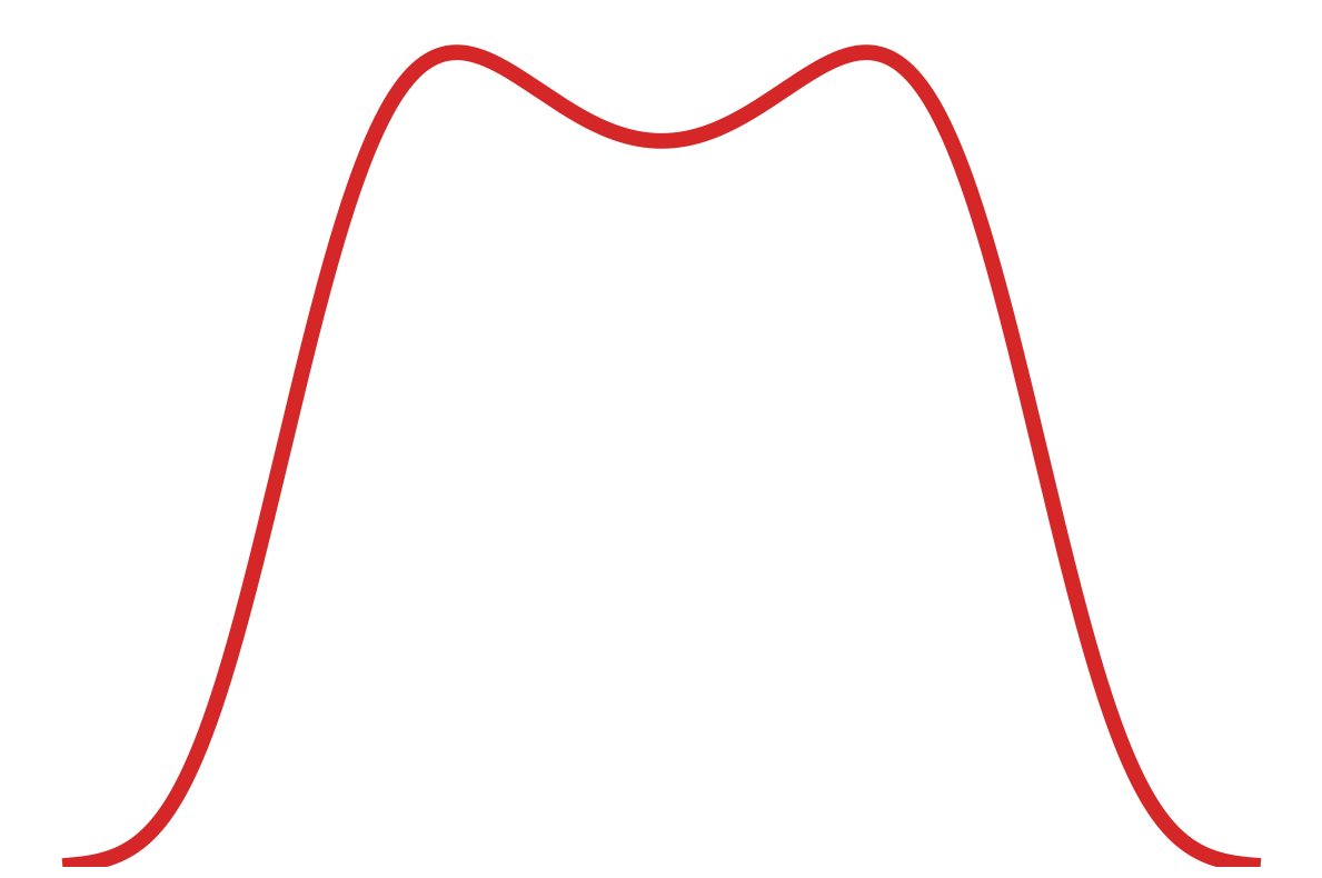
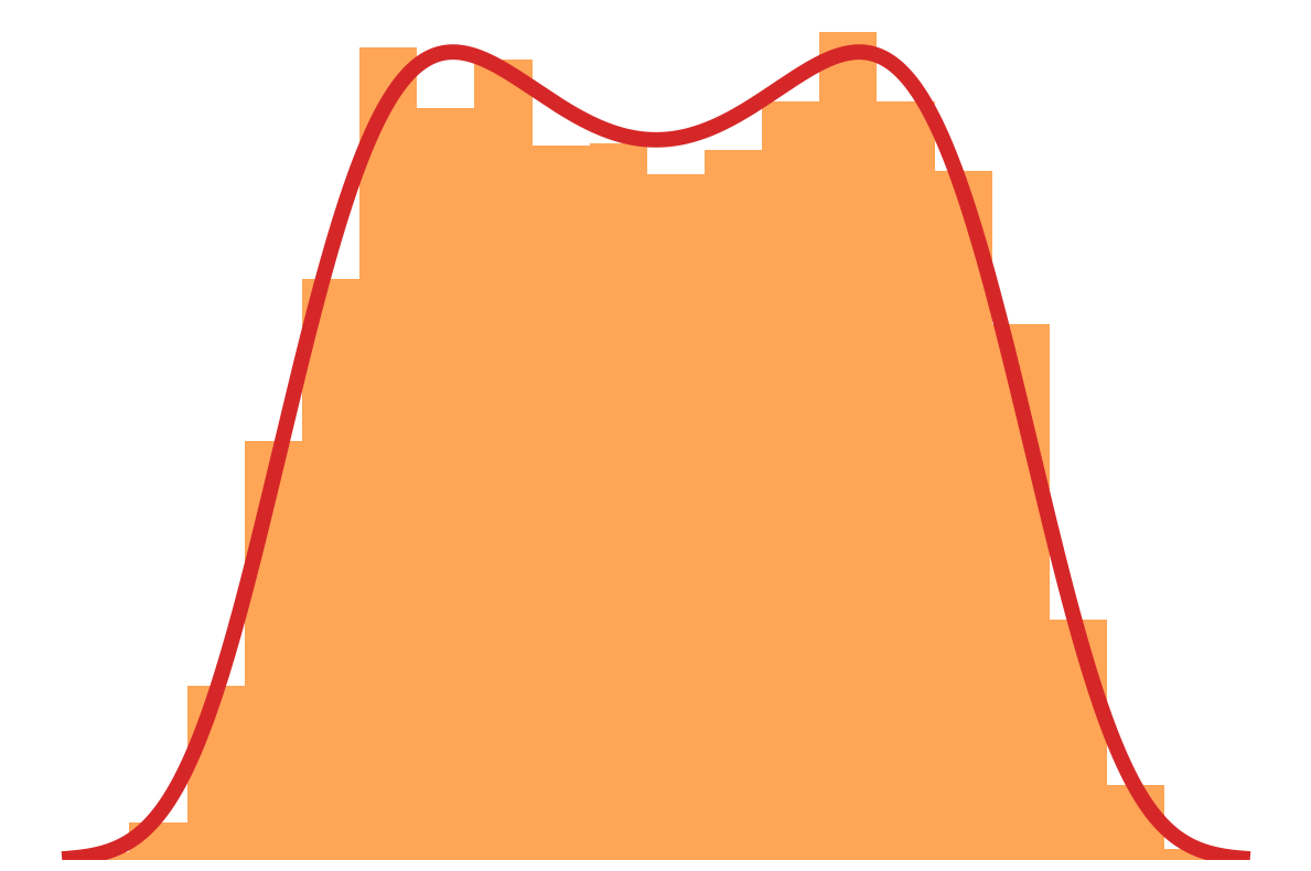
Now let's build a cosmological model!
-
Prior on
- cosmology
- initial field
-
biases
- LPT+PM displacement
- RSD displacement
- Apply Lagrangian bias
- Likelihood of observation

What does it look like?
- parameters, huge!
- We need inference methods that can scale to high dimensions
Sampling
Now that you can score...
Always Bayes
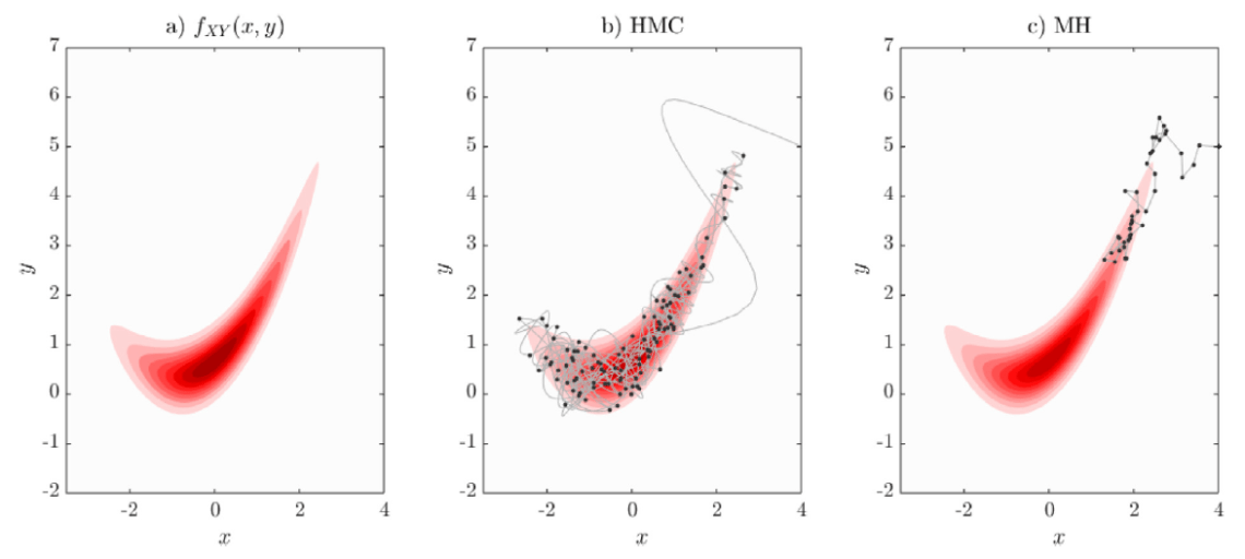
Random Walk Metropolis-Hasting
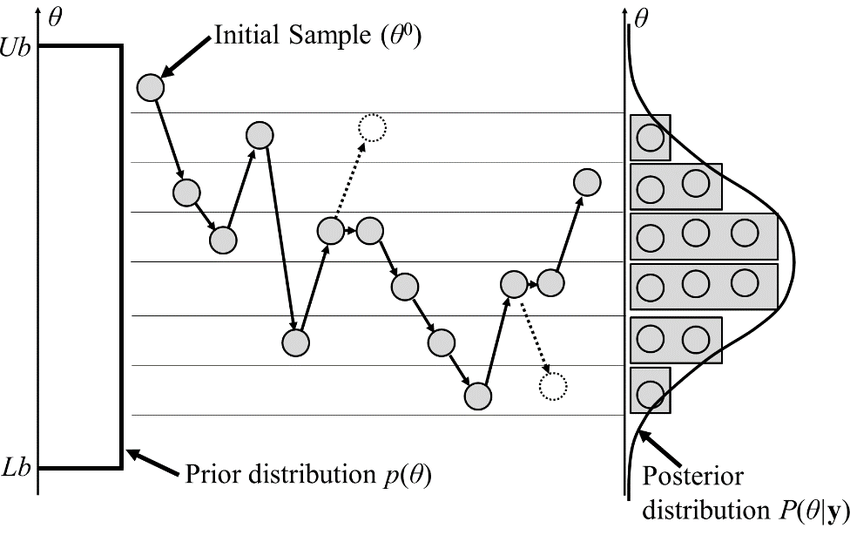
- Basic MCMC sampler
- Proposal agnostic on the target distribution
- so can't do big steps or will reject a lot, cf. demo
Let's use the score: Langevin dynamics
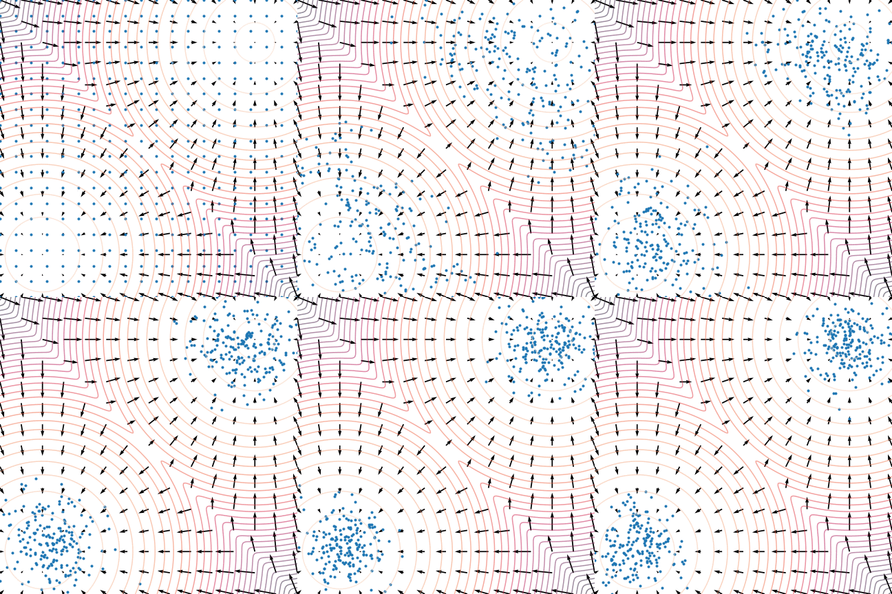
- Score provides local information
- it's the direction of increasing probability
- so let's flow with the (gradient) flow
$$\quad {\displaystyle {d {z}}=\nabla \log p (z , x_0)dt+{\sqrt {2}}{d {W}}}$$

Not good enough? Let's heat things up
- Thanks to score, samples are guided towards high density regions
- But when still in low density regions, score helps less...
- Idea: smooth target distribution, then slowly decrease smoothing
- procedure called annealing
- can be implemented in several ways

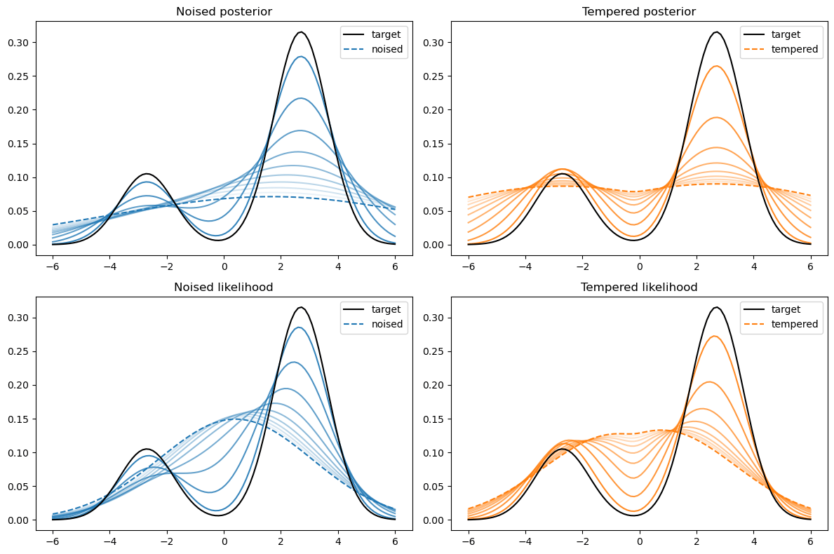
Not good enough? Let's heat things up
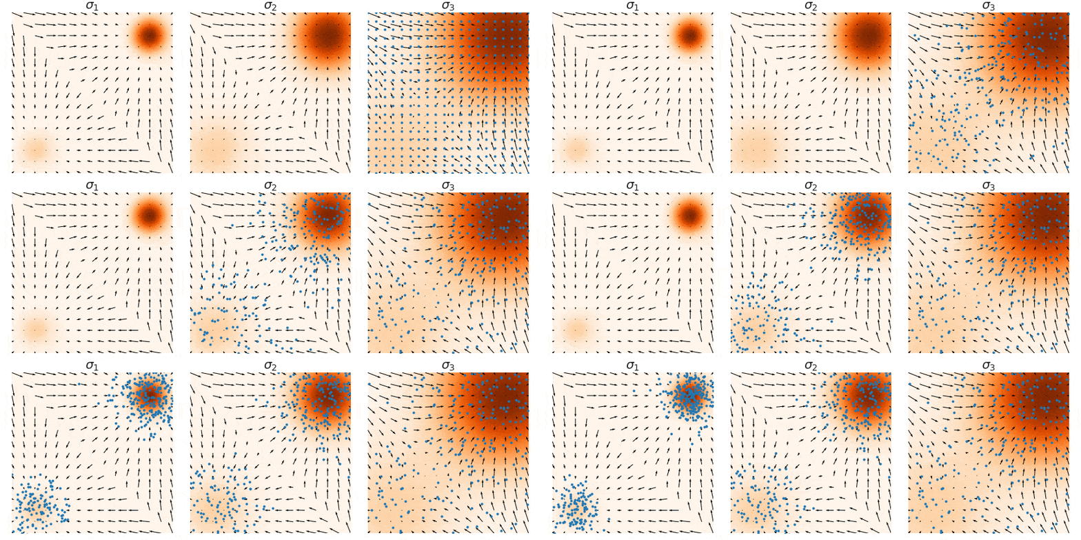
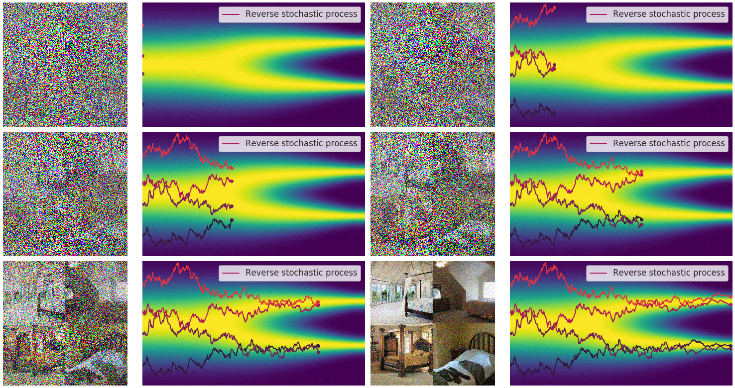
- Thanks to score, MCs are guided towards high density regions
- But when still in low density regions, score helps less...
- Idea: smooth target distribution, then slowly decrease smoothing
- procedure called annealing
- can be implemented in several ways
- So annealing looks like:
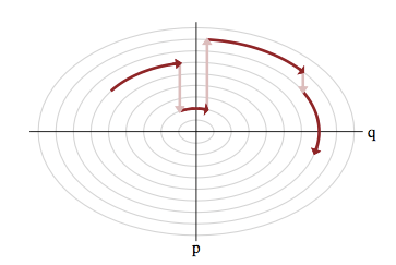
Use the score (again): Hamiltonian Monte Carlo
- To travel farther, add inertia
- augment the sampling space by a momentum space
- at each step sample a momentum
- follow the Hamiltonian dynamic
- Way less correlated than MH, cf. demo
Model Inference
Where model and sampler finally meet
Benchmarking samplers
- Plenty of samplers proposed for field-level inference
-
Hamiltonian Monte Carlo (HMC)
-
HMCGibbs
-
No-U-Turn Sampler (🥜)
-
MicroCanonical Langevin Monte Carlo (MCLMC)
-
Variational self-Boosted Sampling (VBS)
-
Metropolis-Adjusted Langevin Algorithm (MALA)
-
...
-
currently working on a custom version of "Continuously Annealed Langevin Algorithm"
-
"Continuously Annealed Langevin Algorithm"
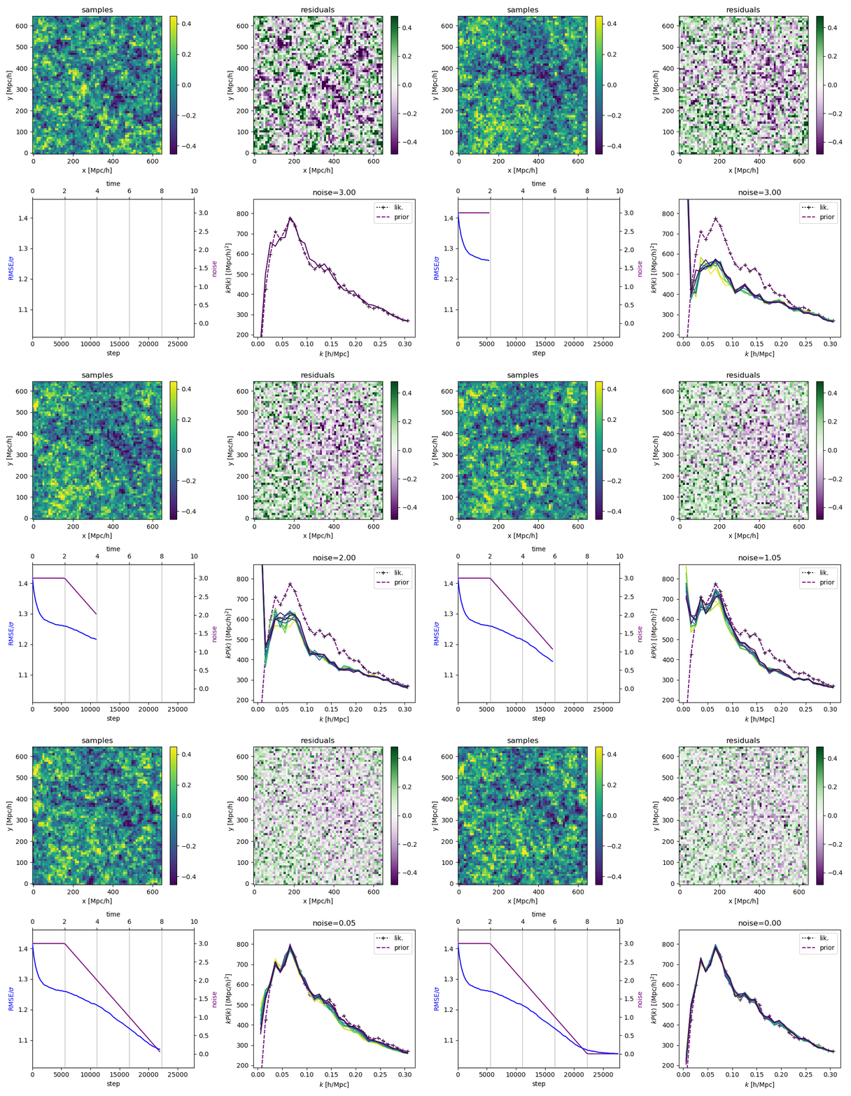
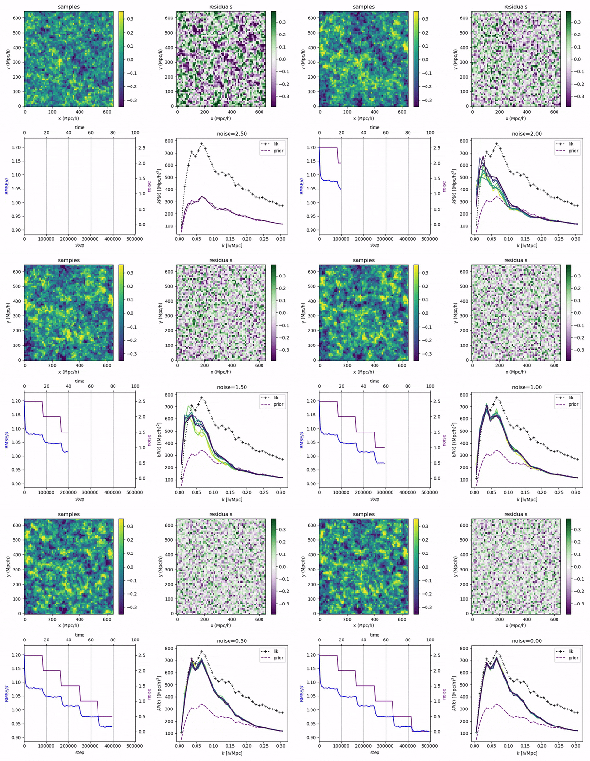
- Idea: a custom annealed Langevin
- continuously anneal target distribution, e.g.
$$p_{s}(z,x_0) := \mathcal N(x_0 \mid f(z), \Sigma + s^2 I) \, p(z)$$ - solve SDE $${\displaystyle {d {z}}=\nabla \log p_{s(t)} (z , x_0)dt+{\sqrt {2}}{d {W}}}$$
- optimize annealing policy \(s(t)\)?
- continuously anneal target distribution, e.g.
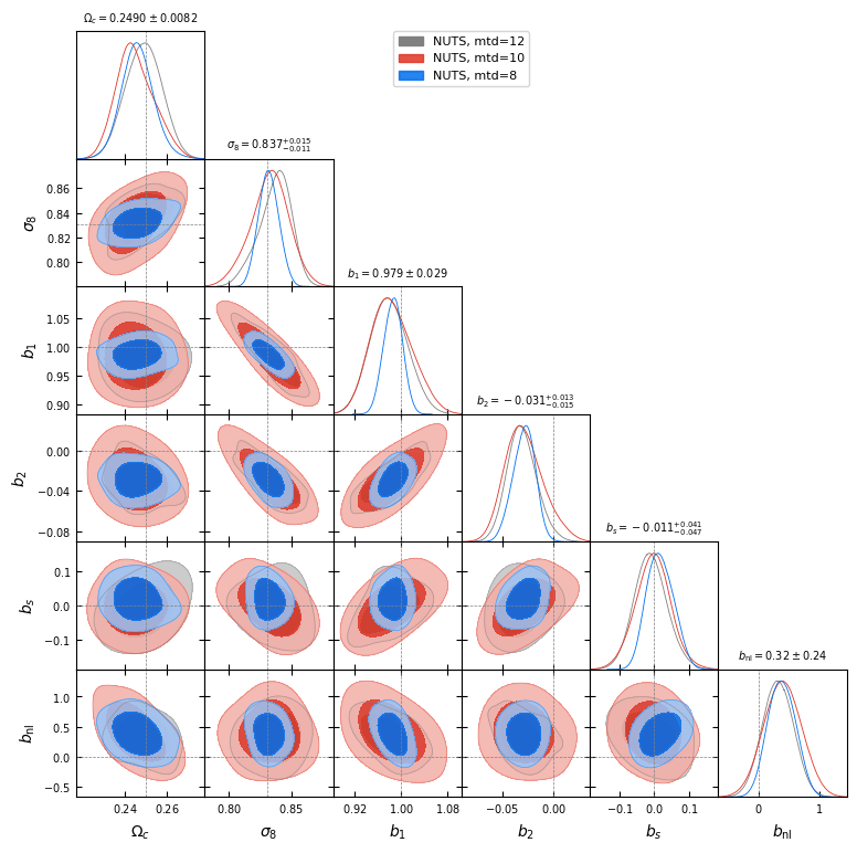
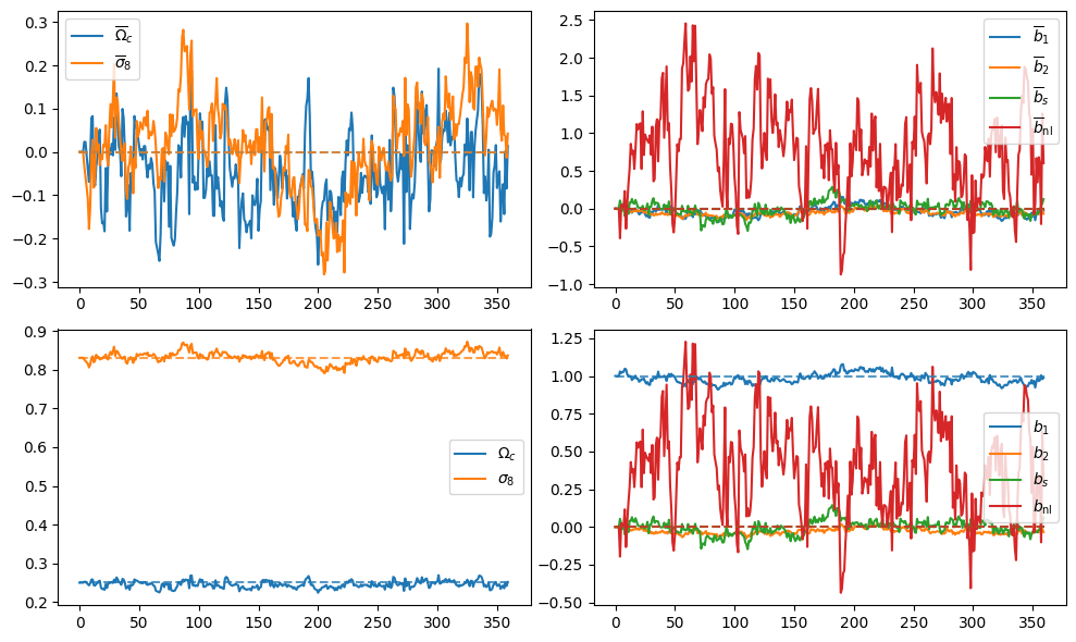
Meanwhile, NUTS
- Preliminary samples from model

What about Implicit Likelihood Inference?
Aims
- Cross-validate model
- Studying Annealed Langevin
- optimal annealing policy?
- SDE solvers?
- translate SDE to PDE?
- Benchmark samplers
- compare to SBI methods