2025Prez

Field-level inference of primordial non-Gaussianity from galaxy redshift surveys

Hugo SIMON,
PhD student supervised by
Arnaud DE MATTIA and François LANUSSE

CoBALt, 2025/06/30

Field-level inference of primordial non-Gaussianity from galaxy redshift surveys

Hugo SIMON,
PhD student supervised by
Arnaud DE MATTIA and François LANUSSE

CoBALt, 2025/06/30

Optimal extraction of primordial non-Gaussian signal from galaxy redshift survey

Hugo SIMON,
PhD student supervised by
Arnaud DE MATTIA and François LANUSSE

Sesto, 2025/07/17

Field-level inference of primordial non-Gaussianity from galaxy redshift surveys

Hugo SIMON,
PhD student supervised by
Arnaud DE MATTIA and François LANUSSE

CSI, 2025/09/02

Field-level analysis of primordial non-Gaussianity with DESI tracers

Hugo SIMON,
PhD student supervised by
Arnaud DE MATTIA and François LANUSSE

PNG Meeting, 2025/06/18

The universe recipe (so far)

$$\frac{H}{H_0} = \sqrt{\Omega_r + \Omega_b + \Omega_c+ \Omega_\kappa + \Omega_\Lambda}$$

instantaneous expansion rate

energy content

Cosmological principle + Einstein equation

+ Inflation

$\delta_L \sim \mathcal G(0, \mathcal P)$

$\sigma_8:= \sigma[\delta_L * \boldsymbol 1_{r \leq 8}]$

initial field

primordial power spectrum

std. of fluctuations smoothed at $8 \text{ Mpc}/h$

$\Omega := \{ \Omega_m, \Omega_\Lambda, H_0, \sigma_8, f_\mathrm{NL},...\}$

Linear matter spectrum

Structure growth

Cosmological modeling and inference

$\Omega$

$\delta_L$

$\delta_g$

inference

DESI+2024

$\Omega$

$\delta_g$

Cosmological inference

DESI+2024

$\Omega$

$P$

$\Omega := \{ \Omega_m, \Omega_\Lambda, H_0, \sigma_8, f_\mathrm{NL},...\}$

inference

$P$

$\Omega$

$\delta_L$

$\delta_g$

Cosmological inference

$\Omega := \{ \Omega_m, \Omega_\Lambda, H_0, \sigma_8, f_\mathrm{NL},...\}$

$\Omega$

$\delta_L$

$\delta_g$

inference

$\delta_L$

$\delta_g$

$\Omega$

Cosmological inference

DESI+2024

$\Omega$

$P$

inference

$\Omega := \{ \Omega_m, \Omega_\Lambda, H_0, \sigma_8, f_\mathrm{NL},...\}$

$\Omega$

$\delta_L$

$\delta_g$

$P$

Cosmological inference

$\Omega := \{ \Omega_m, \Omega_\Lambda, H_0, \sigma_8, f_\mathrm{NL},...\}$

$\Omega$

$\delta_L$

$\delta_g$

inference

$\delta_L$

$\delta_g$

$\Omega$

$128^3$ PM on 8GPU:
4h MCLMC vs. $\geq$ 80h HMC

Fast & differentiable model with

Simon+2025

Bayesian inference

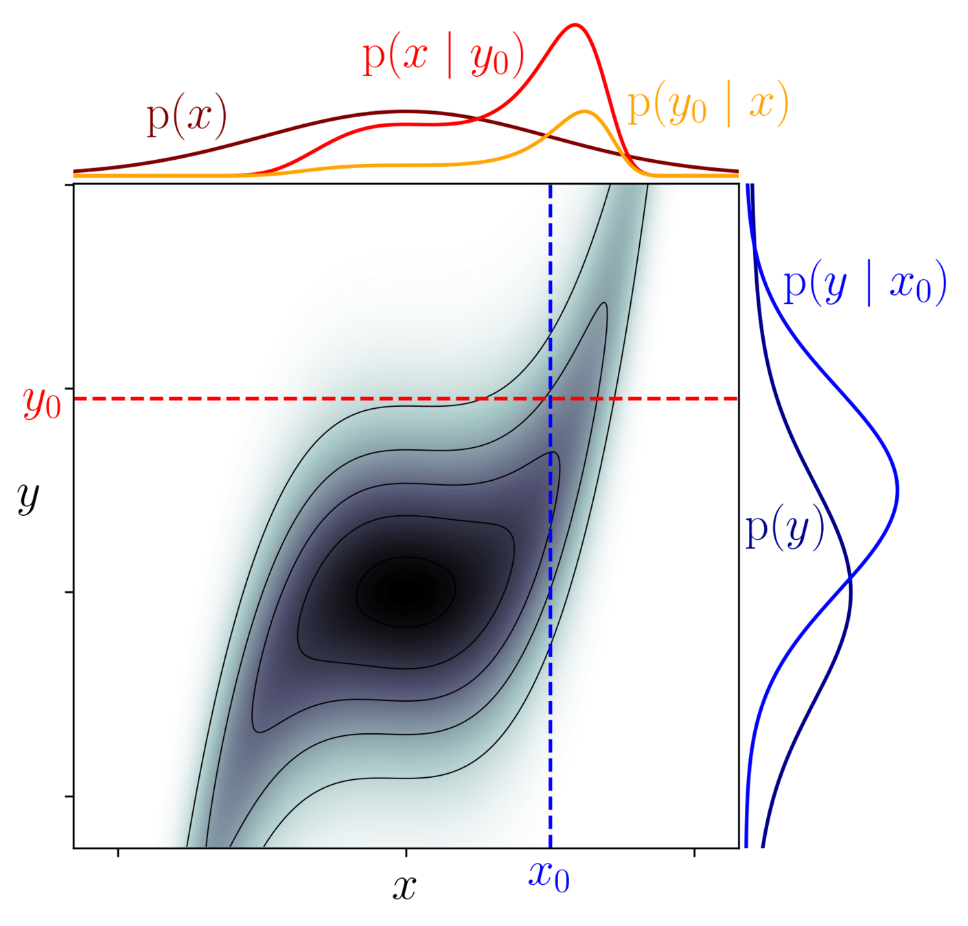
model $=\begin{cases}x \sim \mathcal N(0,1)\\y\mid x \sim \mathcal N(x^3, 1)\end{cases}$

Among all possible worlds $x,y$, restrict to the ones compatible with observation $y_0$:

$$\underbrace{\mathrm p(x \mid y_0)}_{\text{posterior}} = \frac{\overbrace{\mathrm p(y_0 \mid x)}^{\text{likelihood}}}{\underbrace{\mathrm p(y_0)}_{\text{evidence}}}\underbrace{\mathrm p(x)}_{\text{prior}}$$

$x$

$y$

condition

$x$

$y$

$\mathrm{p}(x,y)$

$\mathrm{p}(x \mid y_0)$

Numerically:

Simulate a possible world $x,y$
Assess $x$ credibility by comparing $y$ to $y_0$
Repeat

Please define model

Model: an observation generator, link between latent and observed variables

$F$

$C$

$D$

$E$

$A$

$B$

$G$

Frequentist:

fixed but unknown parameters

Bayesian:

random because unknown

$A$

$B$

$C$

$F$

$D$

$E$

$G$

Represented as a DAG which expresses a joint probability factorization, i.e. conditional dependencies between variables

latent param

latent variable

observed variable

Definitions

evidence/prior predictive: $$\mathrm{p}(y) := \int \mathrm{p}(y \mid x) \mathrm{p}(x)\mathrm d x$$

posterior predictive: $$\mathrm{p}(y_1 \mid y_0) := \int \mathrm{p}(y_1 \mid x) \mathrm{p}(x \mid y_0)\mathrm d x$$

$y$

$x$

Bayes thm

$\sim$

$\underbrace{\mathrm{p}(x \mid y)}_{\text{posterior}}\underbrace{\mathrm{p}(y)}_{\text{evidence}} = \underbrace{\mathrm{p}(y \mid x)}_{\text{likelihood}} \,\underbrace{\mathrm{p}(x)}_{\text{prior}}$

$y$

$x$

Marginalization:

$y$

$x$

$z$

$x$

$y$

$x$

$y$

$x$

Conditioning:

Definitions

$x$

$z$

Marginalization:

$y$

$x$

Conditioning:

evidence/prior predictive: $$\mathrm{p}(y) := \int \mathrm{p}(y \mid x) \mathrm{p}(x)\mathrm d x$$

posterior predictive: $$\mathrm{p}(y_1 \mid y_0) := \int \mathrm{p}(y_1 \mid x) \mathrm{p}(x \mid y_0)\mathrm d x$$

$y$

$x$

Bayes thm

$\sim$

$\underbrace{\mathrm{p}(x \mid y)}_{\text{posterior}}\underbrace{\mathrm{p}(y)}_{\text{evidence}} = \underbrace{\mathrm{p}(y \mid x)}_{\text{likelihood}} \,\underbrace{\mathrm{p}(x)}_{\text{prior}}$

$y$

$x$

$s$

$\Omega$

Cosmology is (sometimes) hard

Probabilistic Programming: Wish List

$\begin{cases}x,y,z \text{ samples}\\\mathrm{p}(x,y,z)\\ U= -\log \mathrm{p}\\\nabla U,\nabla^2 U,\dots\end{cases}$

1. Modeling

e.g. in JAX with $\texttt{NumPyro}$, $\texttt{JaxCosmo}$, $\texttt{JaxPM}$, $\texttt{DISCO-EB}$...

2. DAG compilation

PPLs e.g. $\texttt{NumPyro}$, $\texttt{Stan}$, $\texttt{PyMC}$...

3. Inference

e.g. MCMC or VI with $\texttt{NumPyro}$, $\texttt{Stan}$, $\texttt{PyMC}$, $\texttt{emcee}$...

4. Extract and viz

e.g. KDE with $\texttt{GetDist}$, $\texttt{GMM-MI}$, $\texttt{mean()}$, $\texttt{std()}$...

Physics job

Stats job

auto!

$x$

$z$

$y$

$x$

$y$

DESI2024VI

1

2

3

4

Field-level inference

Summary stat inference

$\Omega$

$s$

$\delta_g$

$\Omega$

$\delta_L$

$s$

marginalize

condition

marginalize

$\Omega$

$s$

$\delta_g$

$\Omega$

$\delta_L$

condition

Two approaches to cosmological inference

Cosmo model

$\mathrm{p}(\Omega,s)$

$\mathrm{p}(\Omega \mid s)$

$\Omega$

$\delta_g$

$\mathrm{p}(\Omega,\delta_L,\delta_g, s)= \mathrm{p}(s \mid \delta_g) \, \mathrm{p}(\delta_g \mid \Omega,\delta_L)\, \mathrm{p}(\delta_L \mid \Omega)\, \mathrm{p}(\Omega)$

$\mathrm{p}(\Omega,\delta_L \mid \delta_g)$

$\mathrm{p}(\Omega \mid \delta_g)$

$\delta_g$

$\Omega$

$\delta_L$

$s$

Two approaches to cosmological inference

Cosmo model

Problem:

$s$ is too simple $\implies$ lossy compression
$s$ is too complex $\implies$ intractable marginalization

The Problem:

high-dimensional integral $$\mathrm{p}(\Omega \mid \delta_g) = \int \mathrm{p}(\Omega, \delta_L \mid \delta_g) \;\mathrm d \delta_L$$
To probe scales of $15\ \mathrm{Mpc}/h$ in DESI volume, $\operatorname{dim}(\delta_L) \simeq 1024^3$

The Promise:

"lossless" explicit inference

Nguyen+2024

Field-level inference

Summary stat inference

We gotta pump this information up

Field-level
CNN...
WST...
Halo, Peak, Void, Split, Hole...
3PCF, Bispectrum
2PCF, Power spectrum
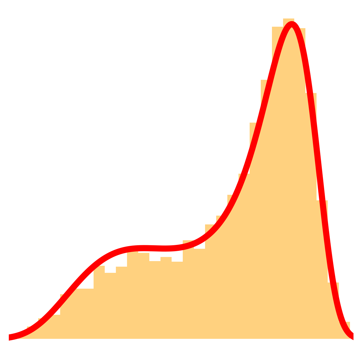
1D-PDF

$$0-$$

$$\mathrm H(\delta_g)-$$

At large scales, matter density field almost Gaussian so power spectrum is almost lossless compression, and is relatively tractable
To prospect smaller non-Gaussian scales, let's use:

Euclid’s view of Perseus

We gotta pump this information up

Field-level
CNN, GNN...
WST, 1D-PDFs, Holes...
Peak, Void, Split, Cluster...
3PCF, Bispectrum
2PCF, Power spectrum

$$0-$$

$$\mathrm H(\delta_g)-$$

At large scales, matter density field is Gaussian so power spectrum is lossless compression, and is relatively tractable
To prospect smaller non-Gaussian scales, let's add:

Euclid’s view of Perseus

all the data
learn the stat
multiscale count
object correlations
more correlations
standard analysis

Bayes, information flavor

$$\boldsymbol{H}(X\mid Y_1)$$

$$\boldsymbol{H}(X)$$

$$\boldsymbol{H}( Y_1)$$

$$\boldsymbol{I}(X; Y_1)$$

$$\boldsymbol{H}( Y_2)$$

$$\boldsymbol{I}(X\mid Y_1; Y_2)$$

$$\boldsymbol{H}(X\mid Y_1,Y_2)$$

$\boldsymbol{H}(X)$ = missing information on $X$ = amount of bits to communicate $X$

$$\boldsymbol{H}(X\mid Y_1)$$

$$\begin{align*}\operatorname{\boldsymbol{H}}(X\mid Y) &= \boldsymbol{H}(Y \mid X) + \boldsymbol{H}(X) - \boldsymbol{H}(Y)\\&= \boldsymbol{H}(X) - \boldsymbol{I}(X;Y) \leq \boldsymbol{H}(X)\end{align*}$$

The summary stats question in cosmology

$$\boxed{\min_s \operatorname{\mathrm{H}}(\Omega\mid s(\delta_g))} = \mathrm{H}(\Omega) - \max_s \mathrm{I}(\Omega ; s(\delta_g))$$

$$\mathrm{H}(\Omega)$$

$$\mathrm{H}(\delta_g)$$

$$\mathrm{H}(\mathcal s_1)$$

$$\mathrm{H}(\mathcal s_2)$$

$$\mathrm{H}(\mathcal P)$$

non-Gaussianities

relevant stat
(low info but high mutual info)

irrelevant stat
(high info but low mutual info)

also a relevant stat
(high info and mutual info)

Which stats are relevant for cosmo inference?

Prior on
- Cosmology $\Omega$
- Initial field $\delta_L$
- EFT Lagrangian parameters $b$
  (Dark matter-galaxy connection)
LSS formation: 2LPT or PM
(BullFrog or FastPM)
Apply galaxy bias
Redshift-Space Distortions
Observational noise

Field-Level Modeling

Fast and differentiable model thanks to ($\texttt{NumPyro}$ and $\texttt{JaxPM}$)

Field-Level Modeling

Fast and differentiable model thanks to ($\texttt{NumPyro}$ and $\texttt{JaxPM}$)

gradients,

they make me:

BaoBan DESI comics by Lamman

See PPL tuto , takeaways:

no more writing likelihood manually
auto-diff a cosmological model

How to N-body-differentiate?

$(\boldsymbol q, \boldsymbol p)$

$\delta(\boldsymbol x)$

$\delta(\boldsymbol k)$

paint*

read*

fft*

ifft*

fft*

*: differentiable, e.g. with via $\texttt{JaxPM}$, in $\mathcal O(n \log n)$

apply forces
to move particles

solve Vlasov-Poisson
to compute forces

$\begin{cases}\dot {\boldsymbol q} \propto \boldsymbol p\\ \dot{\boldsymbol p} = \boldsymbol f \end{cases}$

$\begin{cases}\nabla^2 \phi \propto \delta\\ \boldsymbol f = -\nabla \phi \end{cases} \implies \boldsymbol f \propto \frac{i\boldsymbol k}{k^2} \delta$

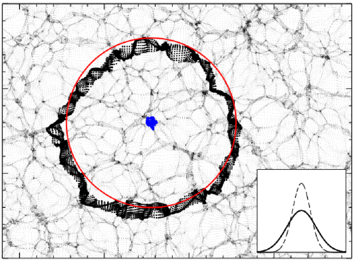
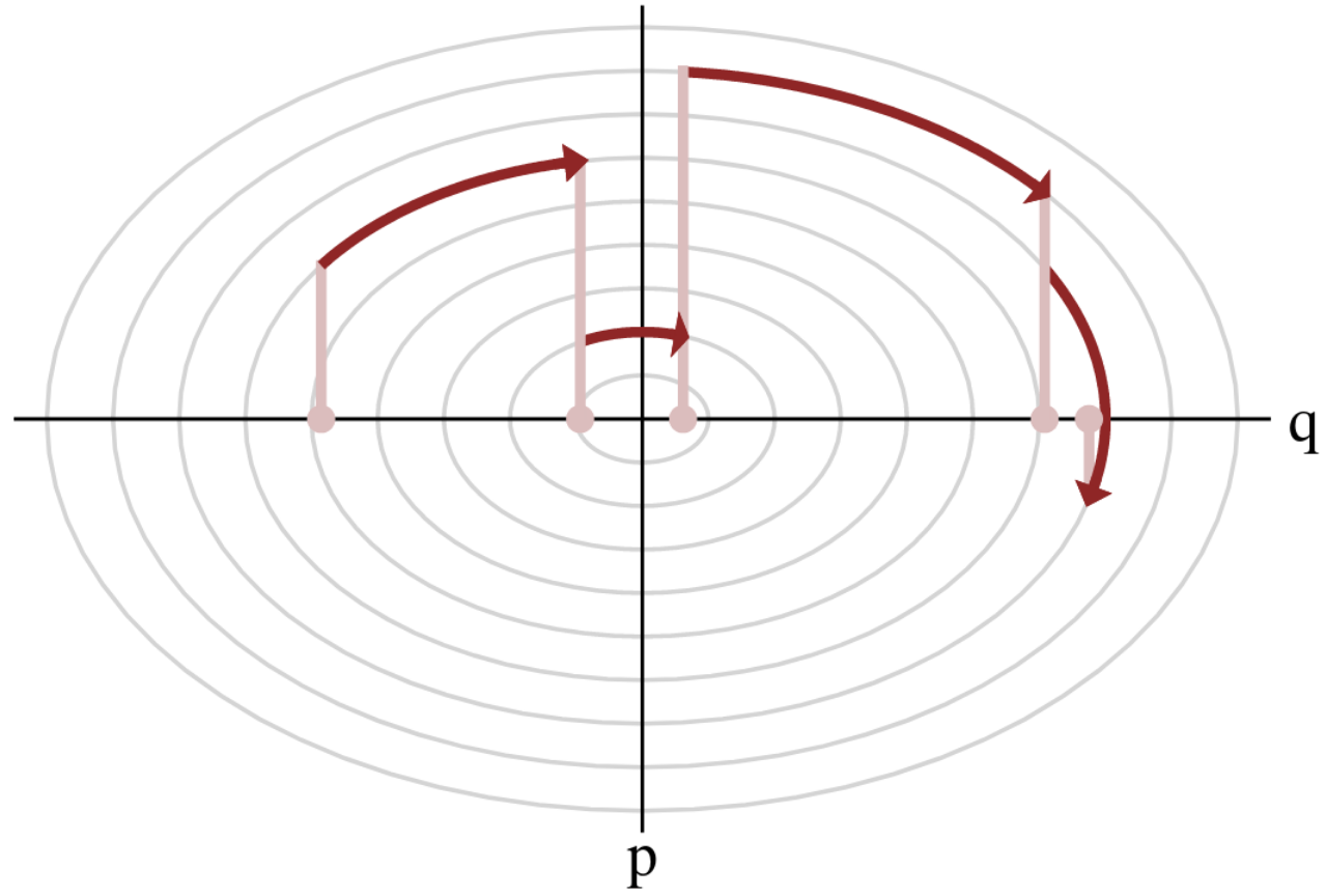
Baryonic Acoustic Oscillations

Eisenstein+2006

Radial mass profile in $\mathrm{cMph}$ of initially point-like overdensity at origin
(Infinite Impulse Response)

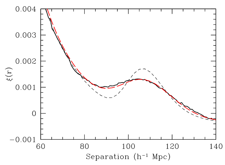
$z=0.3$

BAO observation

$$\begin{cases}\frac{\Delta \theta^\mathrm{fid}}{\Delta \theta} = \frac{D_A}{D_A^\mathrm{fid}}\frac{r_d^\mathrm{fid}}{r_d}=: \alpha_\perp\\\frac{\Delta z^\mathrm{fid}}{\Delta z} = \frac{D_H}{D_H^\mathrm{fid}}\frac{r_d^\mathrm{fid}}{r_d}=: \alpha_\parallel\end{cases}$$

$r_d$

$\Delta \theta$

$\Delta z$

$D_A(z)$

$\Delta \theta = \frac{r_d}{D_A}$

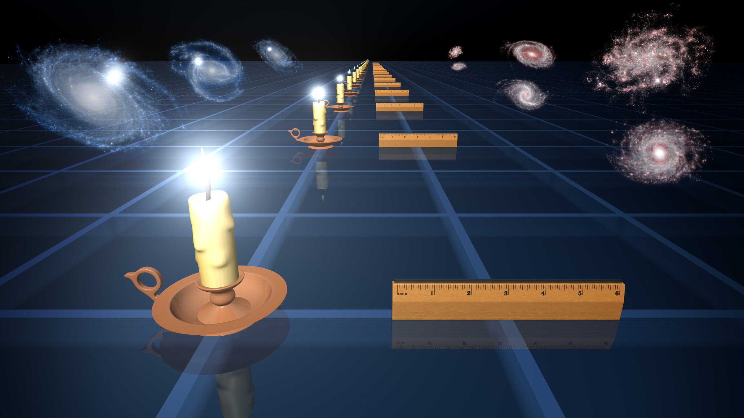
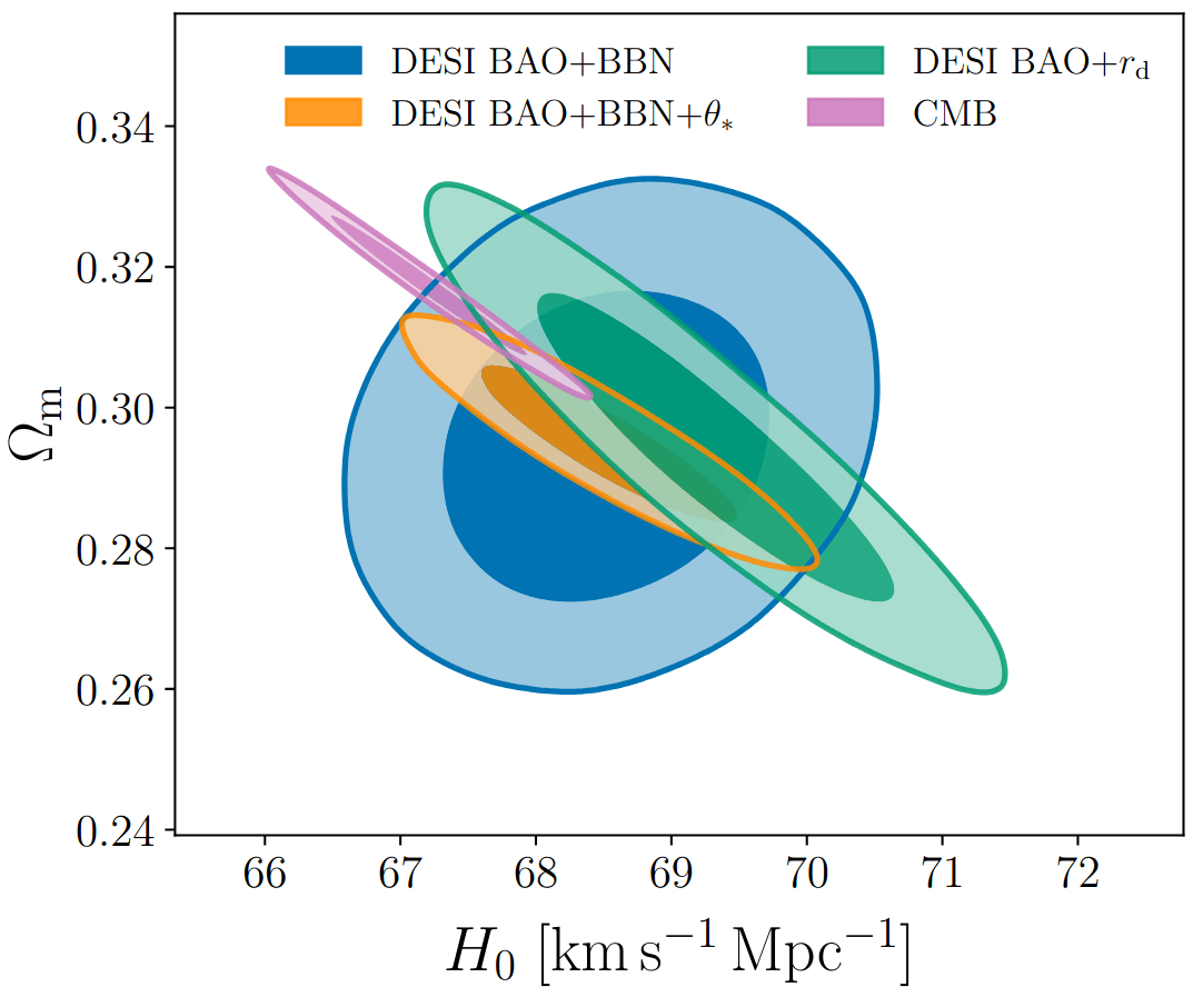
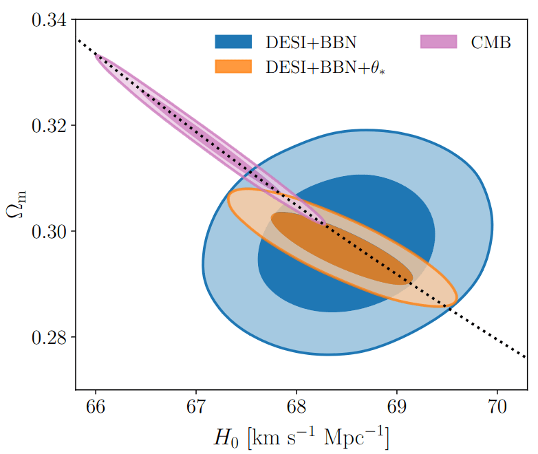
BAO observation

DESI2024

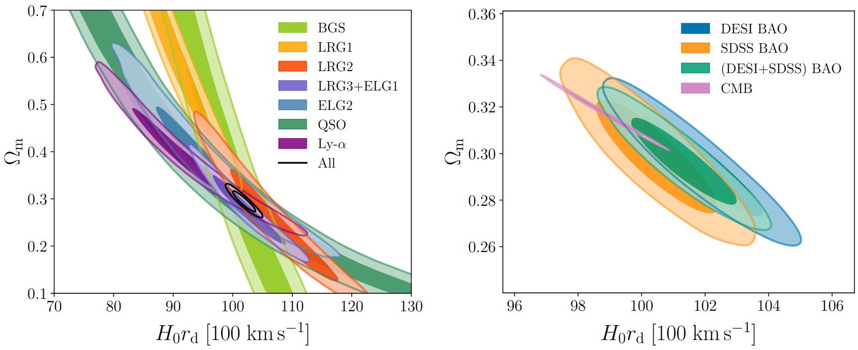
Measuring $\alpha_\perp(z)$ and $\alpha_\parallel(z)$ for multiple $z$ constraints $\Omega_m$ and $H_0 r_d$

$\alpha_\mathrm{iso}$

$\alpha_\mathrm{AP}$

$\alpha_\parallel$

$\alpha_\perp$

$$\begin{cases}\frac{\Delta \theta^\mathrm{fid}}{\Delta \theta} = \frac{D_A}{D_A^\mathrm{fid}}\frac{r_d^\mathrm{fid}}{r_d}=: \alpha_\perp\\\frac{\Delta z^\mathrm{fid}}{\Delta z} = \frac{D_H}{D_H^\mathrm{fid}}\frac{r_d^\mathrm{fid}}{r_d}=: \alpha_\parallel\end{cases}$$

Make Acoustic oscillations Sharp Again

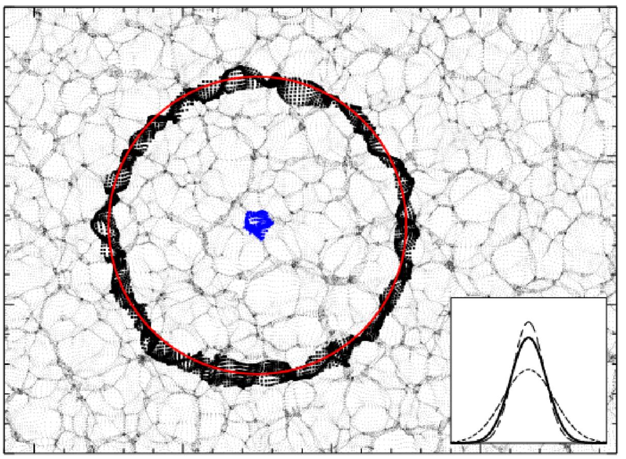
Pictural BAO pre-recon

Pictural BAO post-recon

Padmanabhan+2012

Field-level Inference

$\mathcal H(\boldsymbol q, \boldsymbol p) = U(\boldsymbol q) + \frac 1 2 \boldsymbol p^\top M^{-1} \boldsymbol p$
samples canonical ensemble $$\mathrm p_\text{C}(\boldsymbol q, \boldsymbol p) \propto e^{-\mathcal H(\boldsymbol q, \boldsymbol p)} \propto \mathrm p(\boldsymbol q)\,\mathcal N(\boldsymbol 0, M)$$

HMC (e.g. Neal2011)

Inferring jointly cosmology, bias parameters, and initial matter field

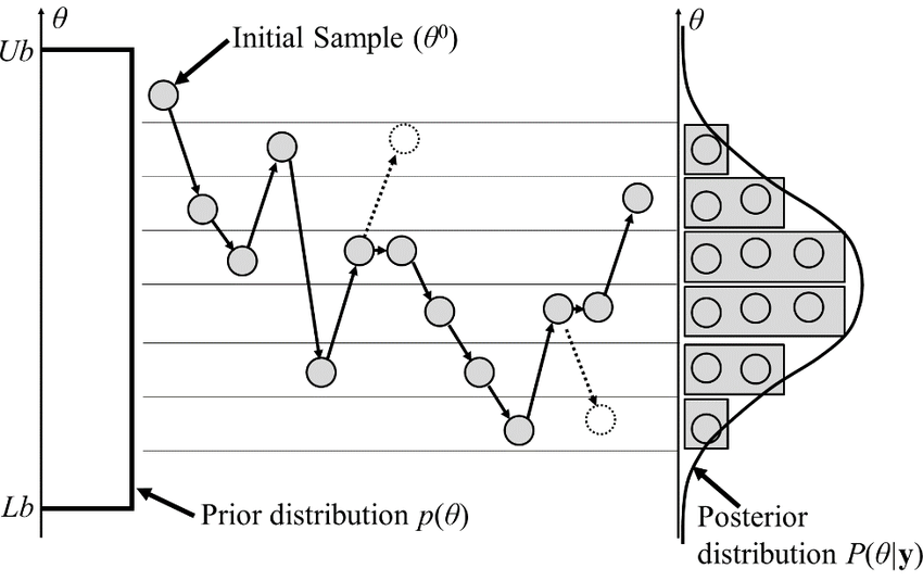
MCMC sampling

High-dimensional sampling is hard

𝓐 𝓭𝓻𝓾𝓷𝓴 𝓶𝓪𝓷 𝔀𝓲𝓵𝓵 𝓯𝓲𝓷𝓭 𝓱𝓲𝓼 𝔀𝓪𝔂 𝓱𝓸𝓶𝓮, 𝓫𝓾𝓽 𝓪 𝓭𝓻𝓾𝓷𝓴 𝓫𝓲𝓻𝓭 𝓶𝓪𝔂 𝓰𝓮𝓽 𝓵𝓸𝓼𝓽 𝓯𝓸𝓻𝓮𝓿𝓮𝓻 ($\mathrm p \approx 0.66$)
🌸 𝓢𝓱𝓲𝔃𝓾𝓸 𝓚𝓪𝓴𝓾𝓽𝓪𝓷𝓲

$-\nabla$

$d \approx 1$

🏠

🚶‍♀️

To maintain constant move-away probability, step-size $\simeq d^{-1/2}$

$d \gg 1$

🪺

🐦

Canonical MCMC samplers

Recipe😋 to sample from $\mathrm p \propto e^{-U}$

take particle with position $\boldsymbol q$, momentum $\boldsymbol p$, mass matrix $M$, and Hamiltonian $$\mathcal H(\boldsymbol q, \boldsymbol p) = U(\boldsymbol q) + \frac 1 2 \boldsymbol p^\top M^{-1} \boldsymbol p$$
follow Hamiltonian dynamics during time $L$
$$\begin{cases} \dot {{\boldsymbol q}} = \partial_{\boldsymbol p}\mathcal H = M^{-1}{{\boldsymbol p}}\\ \dot {{\boldsymbol p}} = -\partial_{\boldsymbol q}\mathcal H = - \nabla U(\boldsymbol q) \end{cases}$$and refresh momentum $\boldsymbol p \sim \mathcal N(\boldsymbol 0,M)$
usually, perform Metropolis adjustment
this samples canonical ensemble $$\mathrm p_\text{C}(\boldsymbol q, \boldsymbol p) \propto e^{-\mathcal H(\boldsymbol q, \boldsymbol p)} \propto \mathrm p(\boldsymbol q)\,\mathcal N(\boldsymbol 0, M)$$

gradient guides particle toward high density sets

scales poorly with dimension

must average over all energy levels

Hamiltonian Monte Carlo (e.g. Neal2011)

Microcanonical MCMC samplers

Recipe😋 to sample from $\mathrm p \propto e^{-U}$

take particle with position $\boldsymbol q$, momentum $\boldsymbol p$, mass matrix $M$, and Hamiltonian $$\mathcal H(\boldsymbol q, \boldsymbol p) = \frac {\boldsymbol p^\top M^{-1} \boldsymbol p} {2 m(\boldsymbol q)} - \frac{m(\boldsymbol q)}{2} \quad ; \quad m=e^{-U/(d-1)}$$
follow Hamiltonian dynamics during time $L$
$$\begin{cases} \dot{\boldsymbol q} = M^{-1/2} \boldsymbol u\\ \dot{\boldsymbol u} = -(I - \boldsymbol u \boldsymbol u^\top) M^{-1/2} \nabla U(\boldsymbol q) / (d-1) \end{cases}$$ and refresh $\boldsymbol u \leftarrow \boldsymbol z/ \lvert \boldsymbol z \rvert \quad ; \quad \boldsymbol z \sim \mathcal N(\boldsymbol 0,I)$
usually, perform Metropolis adjustment
this samples microcanonical/isokinetic ensemble $$\mathrm p_\text{MC}(\boldsymbol q, \boldsymbol u) \propto \delta(H(\boldsymbol q, \boldsymbol u)) \propto \mathrm p (\boldsymbol q) \delta(|\boldsymbol u|^2 - 1)$$

single energy/speed level

let's try avoiding that

gradient guides particle toward high density sets

MicroCanonical HMC (Robnik+2022)

Canonical/Microcanonical MCMC samplers

$\mathcal H(\boldsymbol q, \boldsymbol p) = \frac {\boldsymbol p^\top M^{-1} \boldsymbol p} {2 m(\boldsymbol q)} - \frac{m(\boldsymbol q)}{2} \quad ; \quad m:=e^{-U/(d-1)}$
samples microcanonical/isokinetic ensemble $$\mathrm p_\text{MC}(\boldsymbol q, \boldsymbol p) \propto \delta(\mathcal H(\boldsymbol q, \boldsymbol p)) \propto \mathrm p (\boldsymbol q) \delta(\dot{\boldsymbol q}^\top M \dot{\boldsymbol q} - 1)$$

Hamiltonian Monte Carlo (e.g. Neal2011)

MicroCanonical HMC (Robnik+2022)

$\mathcal H(\boldsymbol q, \boldsymbol p) = U(\boldsymbol q) + \frac 1 2 \boldsymbol p^\top M^{-1} \boldsymbol p$
samples canonical ensemble $$\mathrm p_\text{C}(\boldsymbol q, \boldsymbol p) \propto e^{-\mathcal H(\boldsymbol q, \boldsymbol p)} \propto \mathrm p(\boldsymbol q)\,\mathcal N(\boldsymbol 0, M)$$

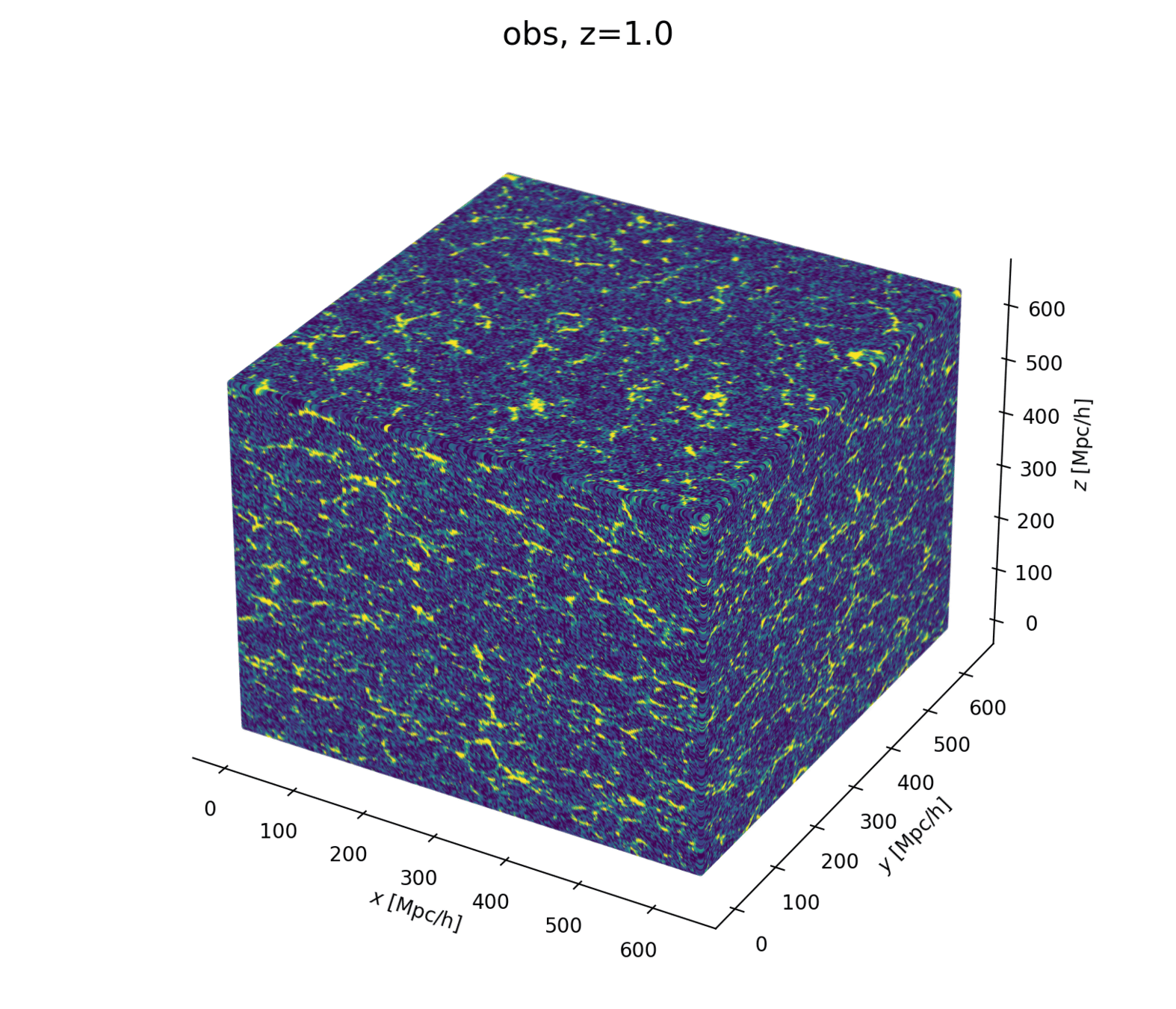
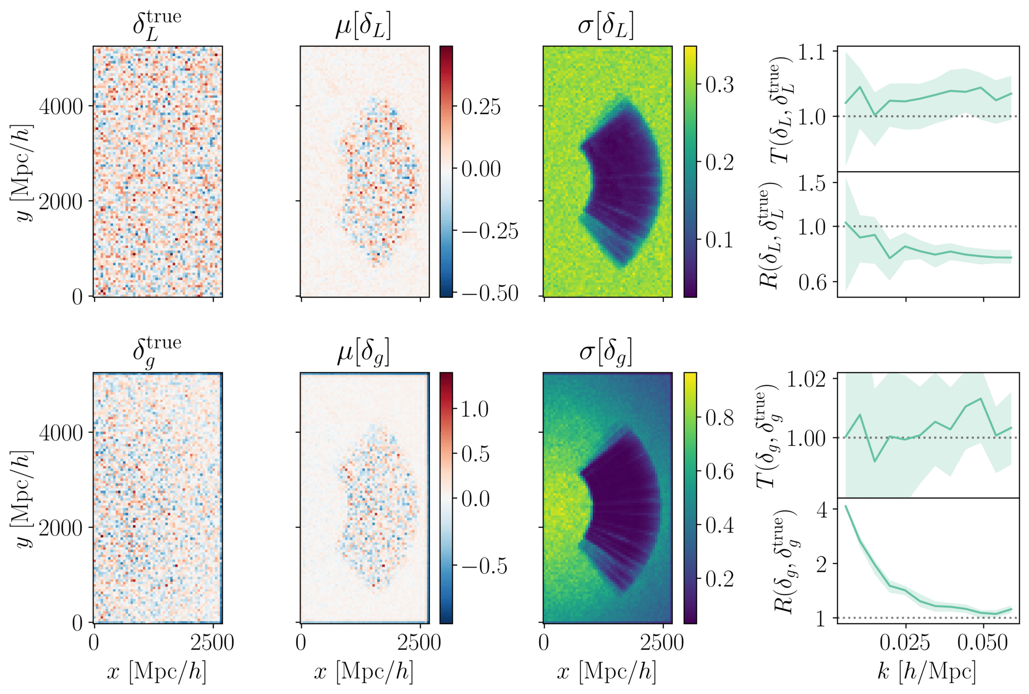
What it looks like

Inferring jointly cosmology, bias parameters, and initial matter field allows full universe history reconstruction

S, Lanusse, de Mattia+2025

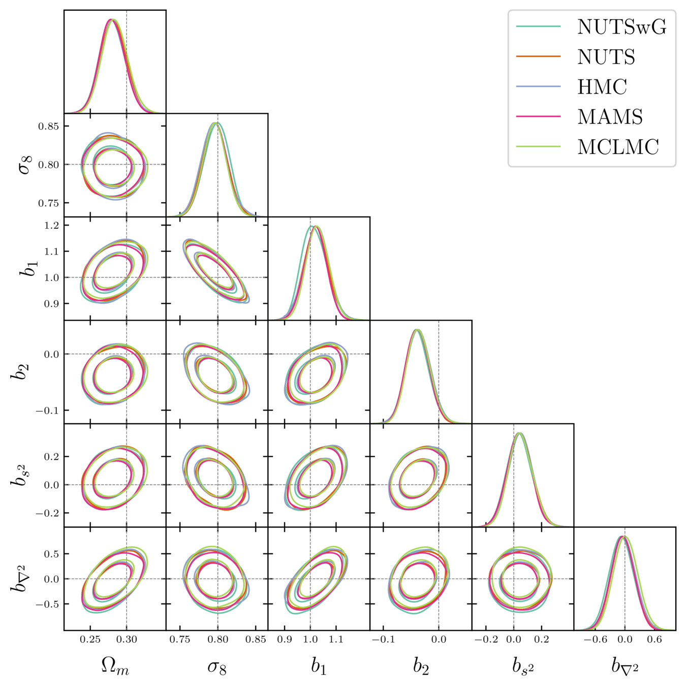
Different samplers and strategies used for field-level (e.g. Lavaux+2018, Bayer+2023). Additional comparisons required.
We provide a consistent benchmark for field-level from galaxy surveys. Build upon $\texttt{NumPyro}$ and $\texttt{BlackJAX}$.

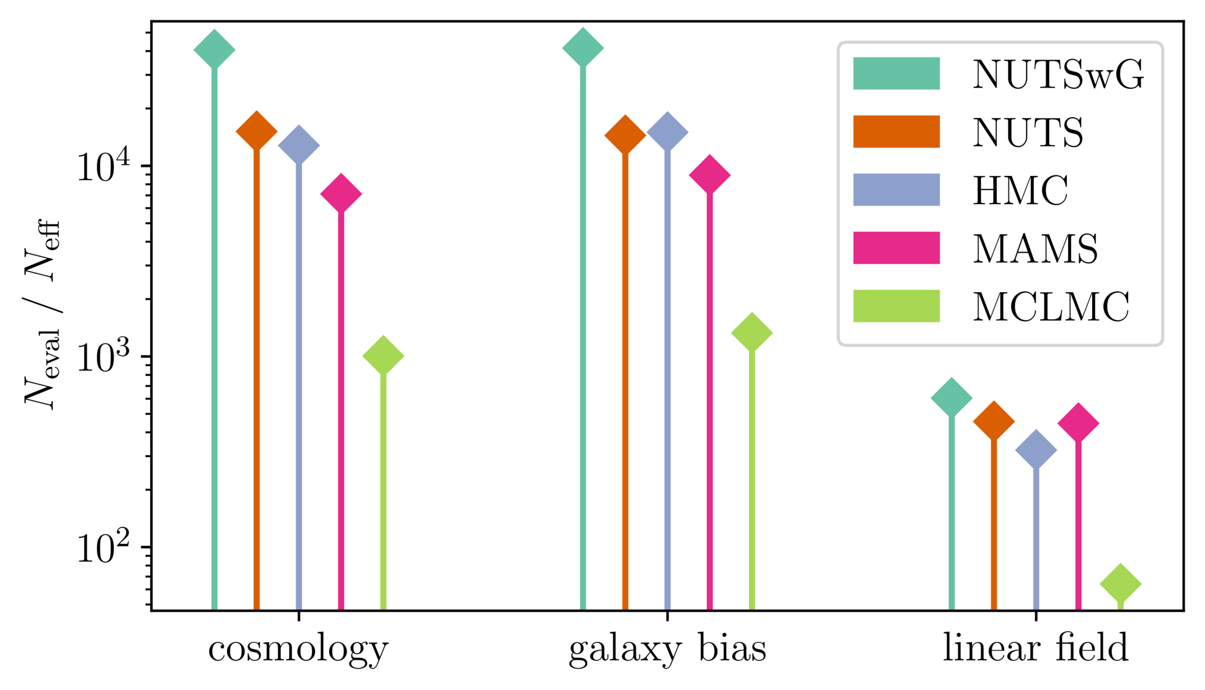
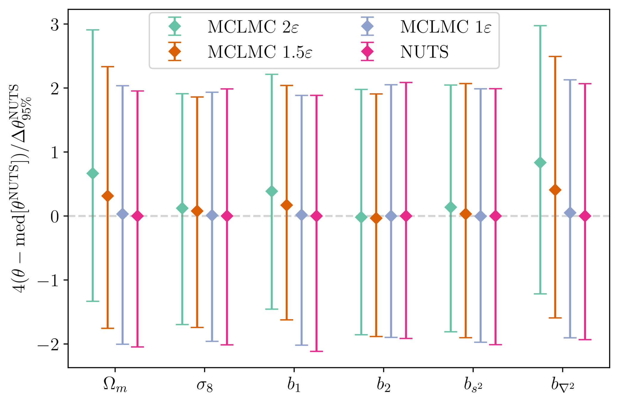
Samplers comparison

= NUTS within Gibbs
= auto-tuned HMC

= adjusted MCHMC
= unadjusted Langevin MCHMC

10 times less evaluations required

Unadjusted microcanonical sampler outperforms any adjusted sampler

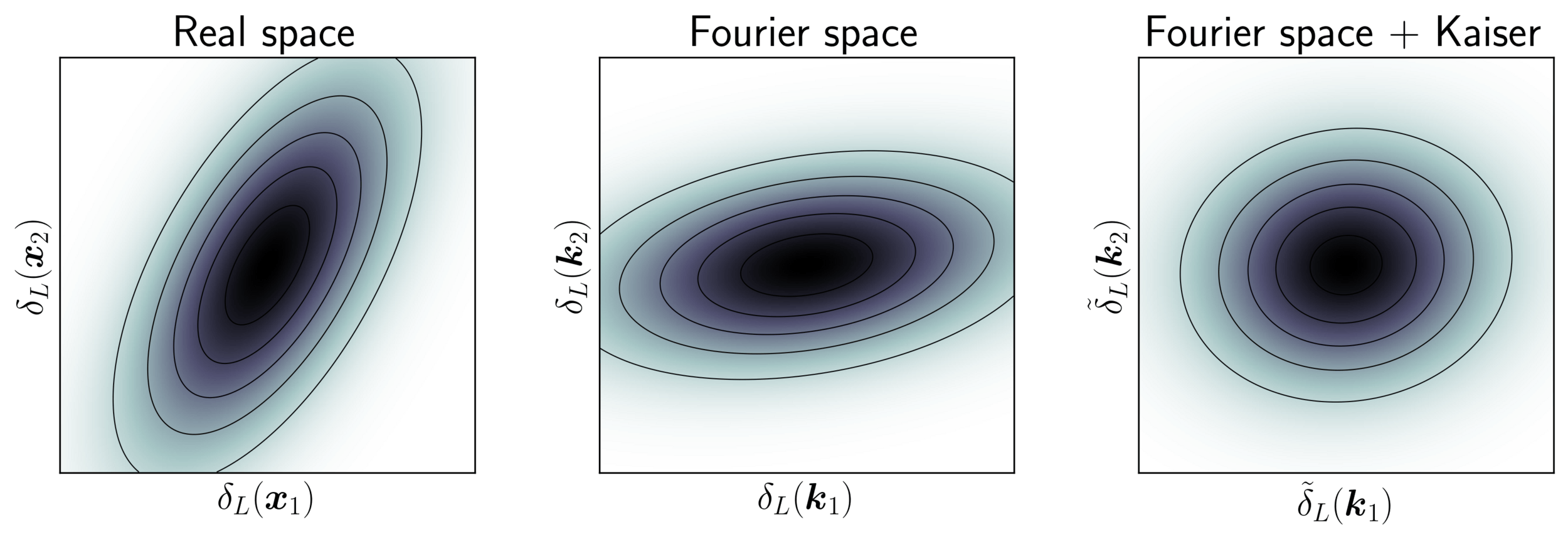
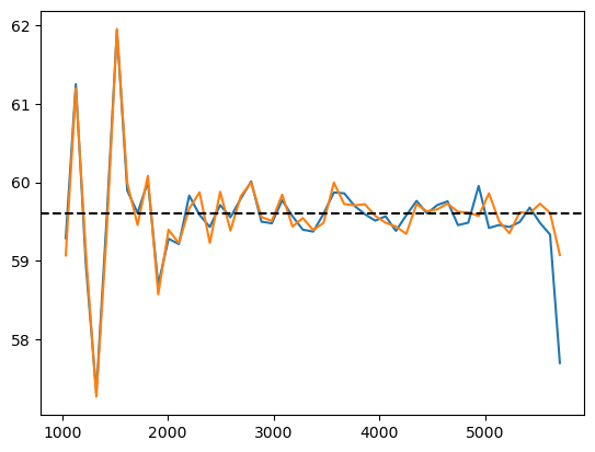
Model preconditioning

Sampling is easier when target density is isotropic Gaussian
The model is reparametrized assuming a tractable Kaiser model:
linear growth + linear Eulerian bias + flat sky RSD + Gaussian noise

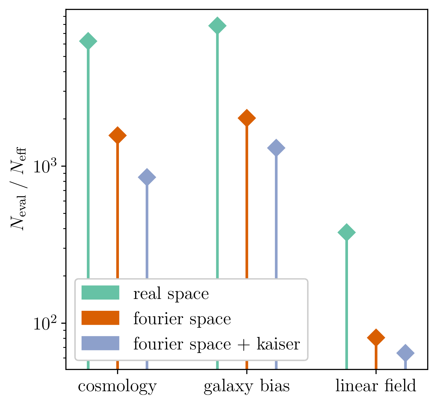
10 times less evaluations required

Benchmark results

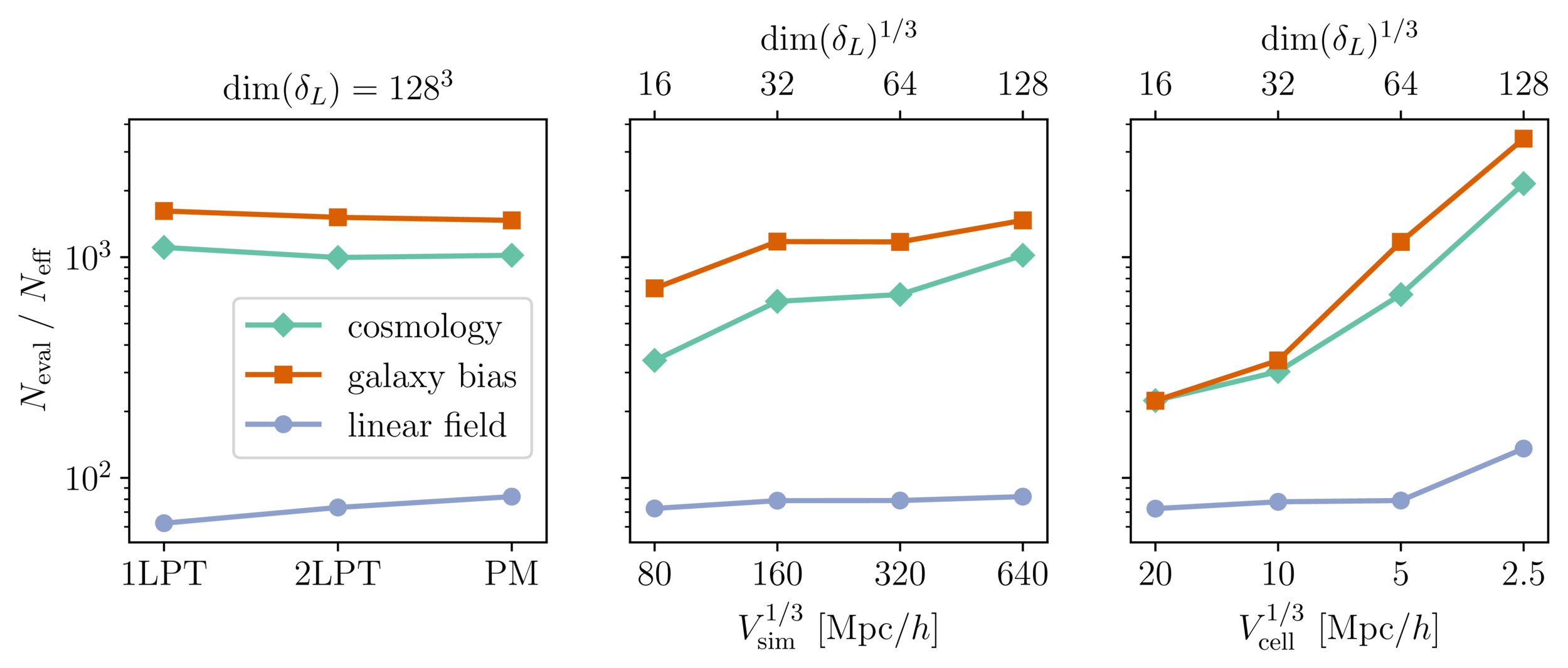
Promising for future inferences, going multi-GPU using JaxDecomp
Code readily available at github.com/hsimonfroy/benchmark-field-level

$128^3$ PM on 8GPU:
4h MCLMC vs. $\geq$80h NUTS

Mildly dependent with respect to formation model and volume

Probing smaller scales could be harder

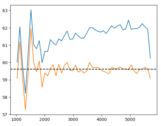
Handling bias in unadjusted MCLMC

Microcanonical dynamics $\implies$ energy should not vary
Numerical integration yields quantifiable errors that can be linked to bias
Stepsize can be tuned to ensure controlled bias, see Robnik+2024

reducing stepsize rapidly brings bias under Monte Carlo error

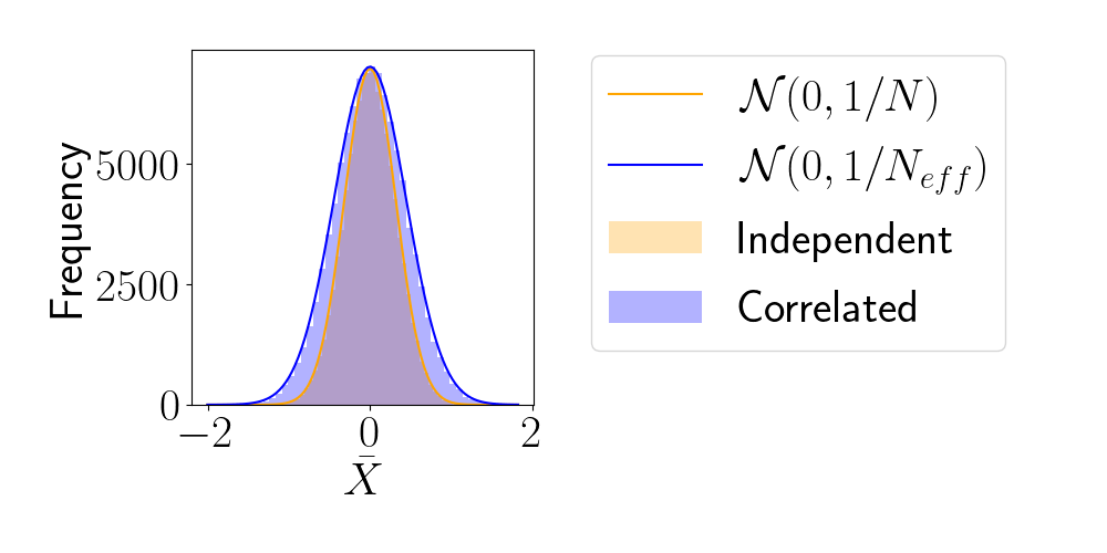
Effective Sample Size (ESS)
- number of i.i.d. samples that yield same statistical power.
- For sample sequence of size $N$ and autocorrelation $\rho$ $$N_\textrm{eff} = \frac{N}{1+2 \sum_{t=1}^{+\infty}\rho_t}$$so aim for as less correlated sample as possible.
Main limiting computational factor is model evaluation (e.g. N-body), so characterize MCMC efficiency by $N_\text{eval} / N_\text{eff}$

Andy Jones

How to compare samplers?

Primordial Non-Gaussianity from galaxies

Local-type PNG is constrained by the induced scale-dependent bias

$\phi_{\mathrm{NL}}=\phi+{\color{purple}f_{\mathrm{NL}}}\phi^{2}$

$\delta(\boldsymbol k)\simeq\left(b_{1}+ b_\phi {\color{purple}f_\mathrm{NL}}k^{-2} \right) \delta_L(\boldsymbol k)$

$f_{\mathrm{NL}}=-3.6_{-9.1}^{+9.0}$

Chaussidon+2024

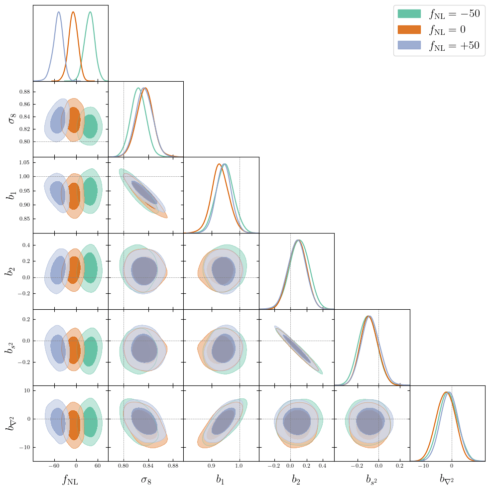
Field-level modeling of PNG

$$\begin{align*}w_g&=1+{\color{purple}b_{1}}\,\delta_{\rm L}+{\color{purple}b_{2}}\delta_{\rm L}^{2}+{\color{purple}b_{s^2}}s^{2}+ {\color{purple}b_{\nabla^2}} \nabla^2 \delta _{\rm L}\\&\quad\quad\! + {\color{purple}b_\phi f_{\rm NL}} \phi + {\color{purple} b_{\phi\delta} f_{\rm NL}} \phi \delta_{\rm L}\\\Delta \boldsymbol q_\parallel &= H^{-1} \dot{\boldsymbol q}_\parallel + {\color{purple}b_{\nabla_\parallel}} \nabla_\parallel \delta_\mathrm{L}\end{align*}$$

$\phi_{\mathrm{NL}}=\phi+{\color{purple}f_{\mathrm{NL}}}\phi^{2}$

Primordial to Linear
Transfer function

modified from Andrews+2024

Galaxy + velocity
bias model

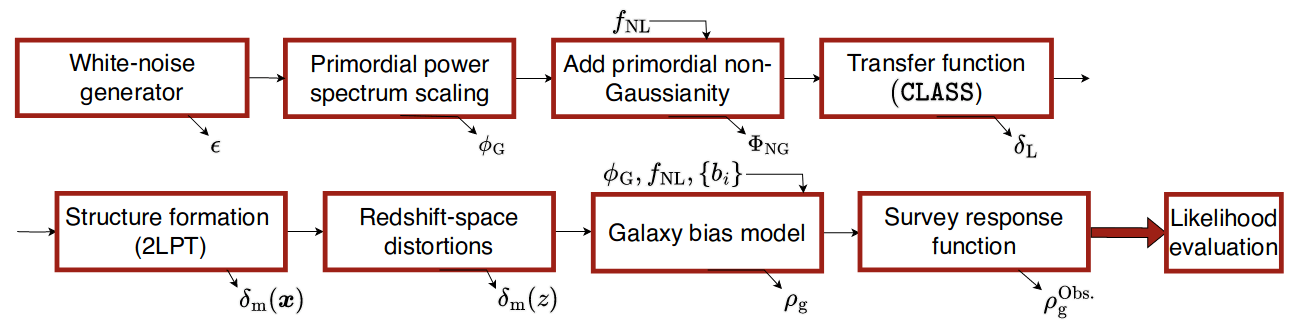
$\boldsymbol q_\mathrm{LPT} \simeq \boldsymbol q_\mathrm{in} + \Psi_\mathrm{LPT}(\boldsymbol q_\mathrm{in}, z(\boldsymbol q_\mathrm{in}))$
one-shot 2LPT light-cone

$n_g^\mathrm{obs}(\boldsymbol q) = (1+\delta_g(\boldsymbol q))\, {\color{purple}\bar n_g(\,r)}\, {\color{blue}W(\boldsymbol q)}\, {\color{purple}\beta_i} {\color{green}T^i(\theta)}$
RIC relax + selection + imag. templates

$\delta_g \sim \mathcal N(\delta_g^\mathrm{det}, \sigma^2)$ with
$\sigma(k) = {\color{purple}\sigma_0}(1+{\color{purple}\sigma_2} k^2 + {\color{purple}\sigma_{\mu2}}(k\mu)^2)$

EFT-based modeling, many scale cuts alleviating discretization effects (see Stadler+2024)

A word on integral constraints

de Mattia+2019

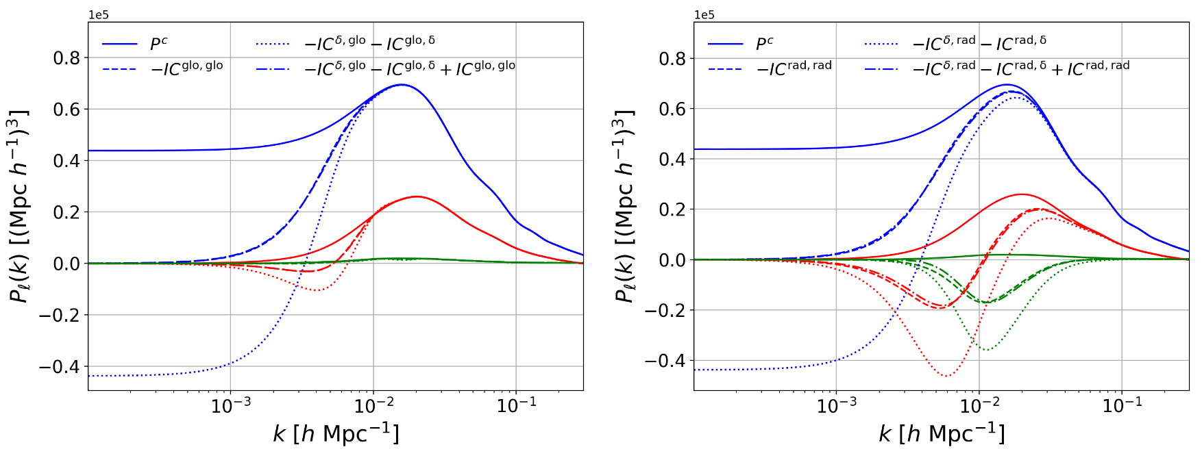
Radial Integral Constraint
$\delta_g \propto n_g - \braket{n_g}\approx n_g - \bar n_g(r)$
i.e. impose $\bar \delta_g(r) = 0$

Global Integral Constraint
$\delta_g \propto n_g - \braket{n_g} \approx n_g - \bar n_g$
i.e. impose $\bar \delta_g = 0$

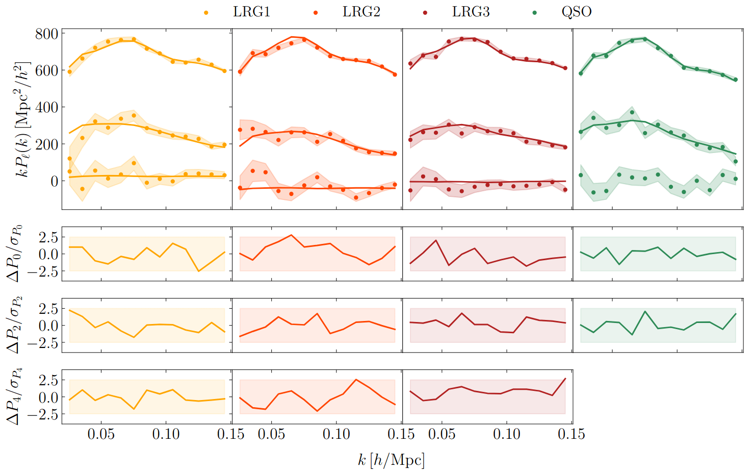
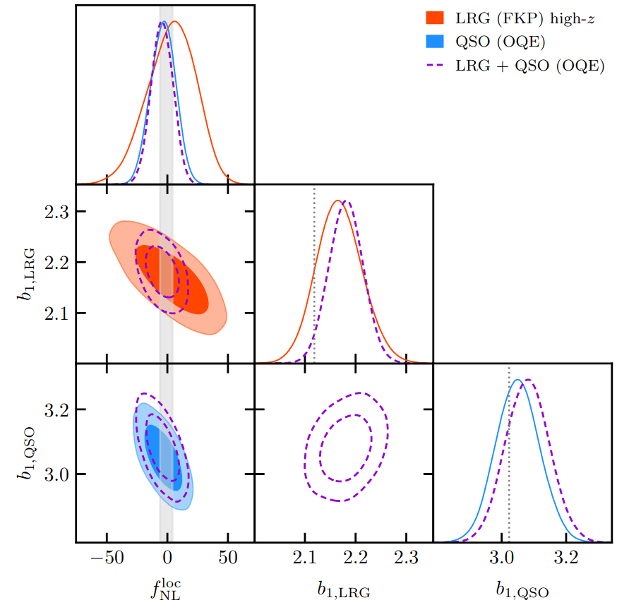
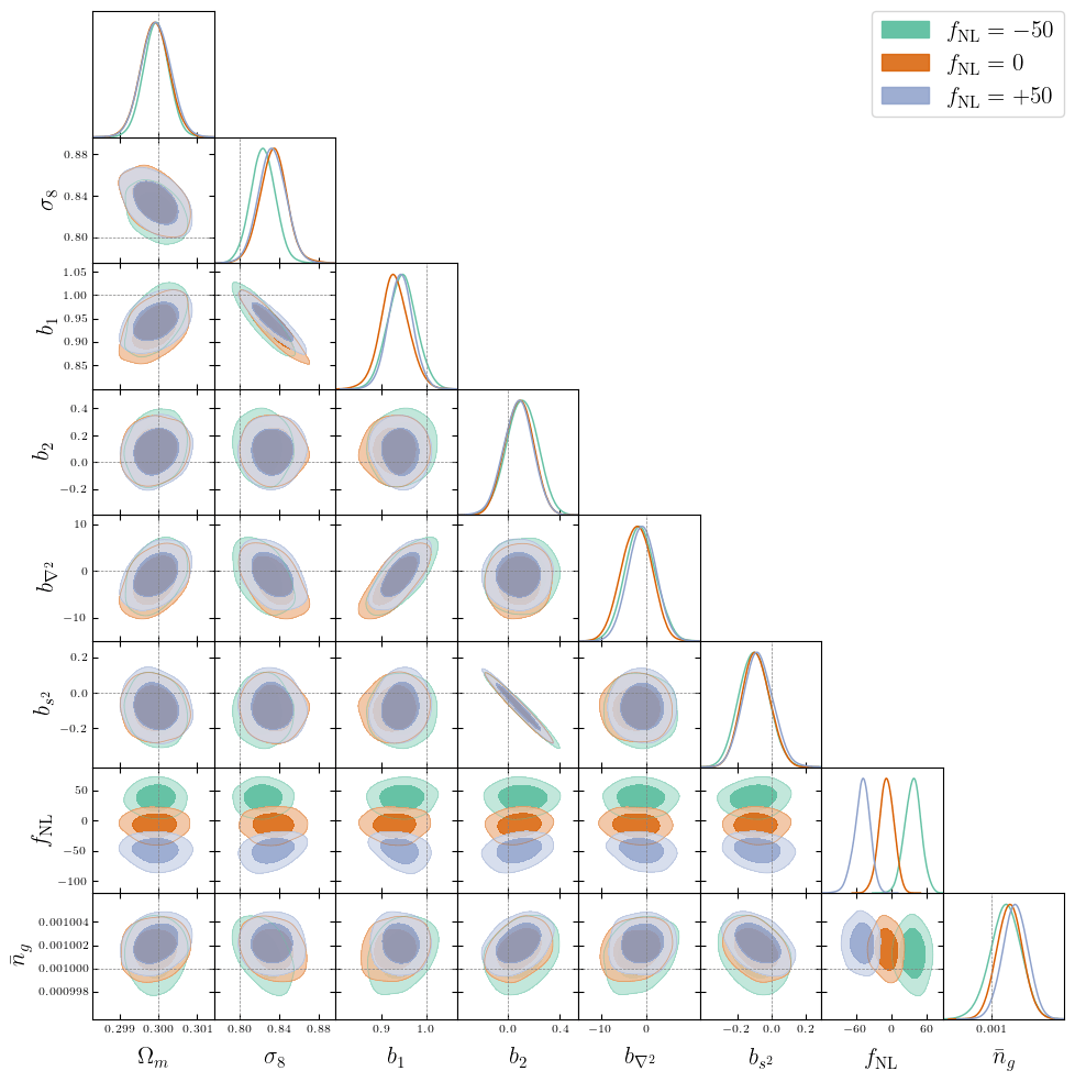
PRELIMINARY

Preliminary results
on LRG SGC footprint

$k_\mathrm{max} \approx 0.04\, [h/\mathrm{Mpc}]$

$\sigma[f_\mathrm{NL}] \approx 20$, consistent with power spectrum analysis (Chaussidon+2024)

Next steps:

EFT model validation (w/o PNG) on AbacusSummit
EFT model validation (w/ PNG) on PNG-Unitsims
Systematics model validation on contaminated mocks
Application to DESI DR1 LRG and QSO

To be answered

3 $f_\mathrm{NL}$ "values" to infer:
- $f_\mathrm{NL}$ in init field, $b_\phi f_\mathrm{NL}$ and $b_{\phi\delta} f_\mathrm{NL}$ in galaxy bias
- "universality" relations robust at field-level?
  $b_\phi = 2 \delta_c (1 + b_1 - p)$ and $b_{\phi \delta} = b_\phi - b_1 + \delta_c b_2$
Redshift varying biases? templates?
- $b_1(z) = a_1 (1+z)^2 + c_1$? $b_2(z)$, $b_s^2(z)$,...?
- Redshift bins? Interpolation?
Max resolution we can robustly + computationally push to
- $k_\mathrm{max} \leq 0.14\, h/\mathrm{Mpc}$?

Where we are

Tally

Currently visiting Montréal in Laurence Perreault-Levasseur team
Talks:
- Optimal cosmo information extraction at Sesto (for Euclid people)
- DESI meeting at Berkeley (for colab)
- CoBALt at Institut Pascal (for inflation theorists)
- Bayesian Deep Learning 3 at APC (for deep learners)
- ED Festival (for particle physicists)
- GDR Cophy 2h tutorial
Papers:
- stat paper at NeurIPS2024 (from master internship)
- Benchmarking Field-Level in review on JCAP
- PNG measurement at the field level in prep
Teaching: Bachelor 2 Biostats (20h) and Master 1 Maths (15) courses at UPsaclay
Formation:
- VSS, Science ethics, Sustainable dev. (Open Science left)
- Euclid summer school

Next steps

Scientific:
- Validation for PNG inference and application to DESI
- Alternative sampling method for field-level inference
- Going Multi-GPU
Manuscript:
- Detailed plan at the end of December, first chapter in January
Looking and applying for postdocs this Autumn,
hence the meetings and visits...

Where we are

Primordial PNG and linear matter field ✔️
Structure formation (2LPT) ✔️
Matter-galaxy connection (EFT) (to validate)
Light-cone, curved-sky, RSD ✔️
Alcock-Paczynski (to correct)
Window, relaxing radial integral constraint ✔️
Systematics (to implement)
Simple likelihood (to correct)
(to replace by EFT likelihood + systematics modeling)

Alcock-Paczynski Problems

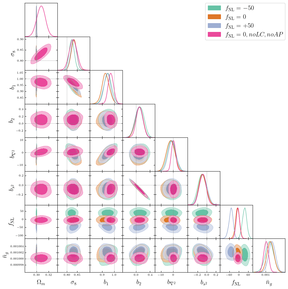
PRELIMINARY RESULTS

$\alpha_\mathrm{iso}$/$\Omega_m$ to well-constrained with AP

Alcock-Paczynski Problems

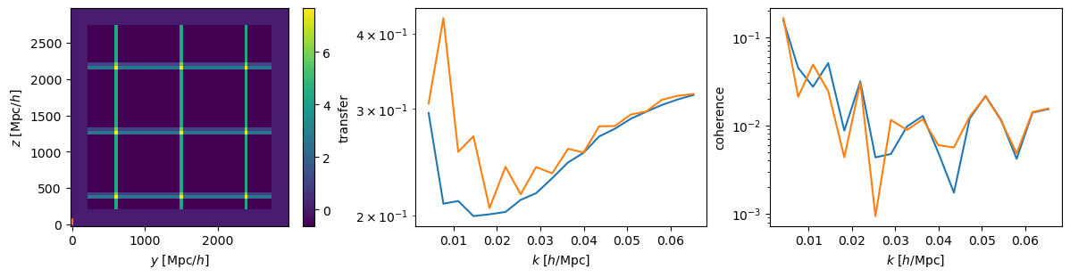
AP modifies simulated tracer density, that we in practice don't know

w/o Jacobian correction w/ Jacobian correction

r [Mpc/h]

n(r)

Did not solved $\alpha_\mathrm{iso}$ constraints. Probably discretization artificats:

Where we are

Next steps:

Correct AP modeling
EFT model validation (w/o PNG) on AbacusSummit
EFT model validation (w/ PNG) on PNG-Unitsims
Systematics modeling

Primordial PNG and linear matter field ✔️
Structure formation (2LPT) ✔️
Matter-galaxy connection (EFT) (to validate)
Light-cone, curved-sky, RSD ✔️
Alcock-Paczynski (to correct)
Window, relaxing radial integral constraint ✔️
Systematics (to implement)
Simple likelihood (to correct)

Some useful programming tools

NumPyro
- Probabilistic Programming Language (PPL)
- Powered by JAX
- Integrated samplers

JAX
- GPU acceleration
- Just-In-Time (JIT) compilation acceleration
- Automatic vectorization/parallelization
- Automatic differentiation

JAX in practice?

GPU accelerate
JIT compile
Vectorize/Parallelize
Auto-diff

import jax.numpy as np
# then enjoy

function = jax.jit(function)
# function is so fast now!

gradient = jax.grad(function)
# too bad if you love chain ruling by hand

vfunction = jax.vmap(function)
pfunction = jax.pmap(function)
# for-loops are for-loosers

Probabilistic Modeling and Compilation

def simulate(seed):
    rng = np.random.RandomState(seed)
    x = rng.randn()
    y = rng.randn() + x**2
    return x, y

from scipy.stats import norm
log_prior = lambda x: norm.logpdf(x, 0, 1)
log_lik = lambda x, y: norm.logpdf(y, x**2, 1)
log_joint= lambda x, y: log_lik(y, x) + log_prior(x)

grad_log_prior = lambda x: x**2
grad_log_lik = lambda x, y: stack([2 * x * (y - x**2), (y - x**2)])
grad_log_joint = lambda x, y: grad_log_lik(y, x) + stack([grad_log_prior(x), zeros_like(y)])
# Hessian left as an exercise...

To fully define a probabilistic model, we need

its simulator
its associated joint log prob
possibly its gradients, Hessian... (useful for inference)

We should only care about the simulator!

$Y$

$X$

$$\begin{cases}X \sim \mathcal N(0,1)\\Y\mid X \sim \mathcal N(X^2, 1)\end{cases}$$

my model on paper

my model on code

What if we modify to fit variances? non-Gaussian dist? Recompute everything? :'(

NumPyro in practice?

def model():
    x = sample('x', dist.Normal(0, 1))
    y = sample('y', dist.Normal(x**3, 1))
    return y

render_model(model, render_distributions=True)

y0 = dict(y=seed(model, 42)())
obs_model = condition(model, y0)
logd_fn = lambda x: log_density(obs_model,(),{},{'x':x})[0]

from jax import jit, vmap, grad
force_vfn = jit(vmap(grad(logd_fn)))

kernel = infer.NUTS(obs_model)
mcmc = infer.MCMC(kernel, n_warmup, n_samples)
mcmc.run(jr.key(43))
samples = mcmc.get_samples()

Probabilistic Programming
JAX machinery
Integrated samplers

Modeling with Numpyro

y_sample = seed(model, 42)()
log_joint = lambda x, y: log_density(model,(),{},{'x':x, 'y':y})[0]

obs_model = condition(model, y_sample)
logp_fn = lambda x: log_density(obs_model,(),{},{'x':x})[0]

def model():
    x = sample('x', dist.Normal(0, 1))
    y = sample('y', dist.Normal(x**2, 1))
    return y

from jax import jit, vmap, grad
force_vfn = jit(vmap(grad(logp_fn)))

Define model as simulator... and that's it
Simulate, get log prob
+JAX machinery
Condition model
And more!

Why care about differentiable model?

Classical MCMCs
- agnostic random moves
  + MH acceptance step
  = blinded natural selection
- small moves yield correlated samples
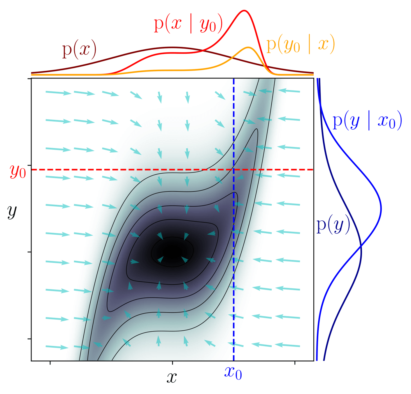
SOTA MCMCs rely on the gradient of the model log-prob, to drive dynamic towards highest density regions

gradient descent
posterior mode

Brownian
exploding Gaussian

Langevin
posterior

+

=

Hamiltonian Monte Carlo (HMC)

To travel farther, add inertia.
- sample particle at position $q$ now have momentum $p$ and mass matrix $M$
- target $\boldsymbol{p}(q)$ becomes $\boldsymbol{p}(q , p) := e^{-\mathcal H(q,p)}$, with Hamiltonian $$\mathcal H(q,p) := -\log \boldsymbol{p}(q) + \frac 1 2 p^\top M^{-1} p$$
- at each step, resample momentum $p \sim \mathcal N(0,M)$
- let $(q,p)$ follow the Hamiltonian dynamic during time length $L$, then arrival becomes new MH proposal.

Variations around HMC

No U-Turn Sampler (NUTS)
- trajectory length $L$ auto-tuned
- samples drawn along trajectory
NUTSGibbs i.e. alternating sampling over parameter subsets.

Why care about differentiable model?

Variations around HMC

No U-Turn Sampler (NUTS)
- trajectory length auto-tuned
- samples drawn along trajectory
NUTSGibbs i.e. alternating sampling over parameter subsets

Model gradient drives sample particles towards high density regions
Hamiltonian Monte Carlo (HMC):
to travel farther, add inertia
Yields less correlated chains

3) Hamiltonian dynamic

1) mass $M$ particle at $q$

2) random kick $p$

1) mass $M$ particle at $q$

3) Hamiltonian dynamic

Hugo SIMON
PhD student supervised by
Arnaud DE MATTIA and François LANUSSE

Field-level Bayesian inference
High-dimensional sampling
Differentiable N-body simulations
Primordial non-Gaussianity from DESI

Hugo SIMON
PhD student at CEA Paris-Saclay, supervised by
Arnaud DE MATTIA and François LANUSSE

Field-level Bayesian inference
High-dimensional sampling
Differentiable N-body simulations
Primordial non-Gaussianity field-level inference from DESI

Thank you!

BaoBan comics

Field-level inference of primordial non-Gaussianity from galaxy redshift surveys

Field-level inference of primordial non-Gaussianity from galaxy redshift surveys

Optimal extraction of primordial non-Gaussian signal from galaxy redshift survey

Field-level inference of primordial non-Gaussianity from galaxy redshift surveys

Field-level analysis of primordial non-Gaussianity with DESI tracers

The universe recipe (so far)

Cosmological modeling and inference

Cosmological inference

Cosmological inference

Cosmological inference

Cosmological inference

Bayesian inference

Please define model

Definitions

Definitions

Cosmology is (sometimes) hard

Probabilistic Programming: Wish List

Two approaches to cosmological inference

Two approaches to cosmological inference

We gotta pump this information up

We gotta pump this information up

Bayes, information flavor

The summary stats question in cosmology

Field-Level Modeling

Field-Level Modeling

How to N-body-differentiate?

Baryonic Acoustic Oscillations

BAO observation

BAO observation

Make Acoustic oscillations Sharp Again

Field-level Inference

MCMC sampling

High-dimensional sampling is hard

Canonical MCMC samplers

Microcanonical MCMC samplers

Canonical/Microcanonical MCMC samplers

What it looks like

Samplers comparison

Model preconditioning

Benchmark results

Handling bias in unadjusted MCLMC

How to compare samplers?

Primordial Non-Gaussianity from galaxies

Field-level modeling of PNG

A word on integral constraints

Preliminary results on LRG SGC footprint

To be answered

Where we are

Tally

Next steps

Where we are

Alcock-Paczynski Problems

Alcock-Paczynski Problems

Where we are

Some useful programming tools

JAX in practice?

Probabilistic Modeling and Compilation

NumPyro in practice?

Modeling with Numpyro

Why care about differentiable model?

Hamiltonian Monte Carlo (HMC)

Why care about differentiable model?

Hugo SIMON PhD student supervised by Arnaud DE MATTIA and François LANUSSE

Hugo SIMON PhD student at CEA Paris-Saclay, supervised by Arnaud DE MATTIA and François LANUSSE

Preliminary results
on LRG SGC footprint

Hugo SIMON
PhD student supervised by
Arnaud DE MATTIA and François LANUSSE

Hugo SIMON
PhD student at CEA Paris-Saclay, supervised by
Arnaud DE MATTIA and François LANUSSE