2026Durham

The universe recipe (so far)

$$\frac{H}{H_0} = \sqrt{\Omega_r + \Omega_b + \Omega_c+ \Omega_\kappa + \Omega_\Lambda}$$

instantaneous expansion rate

energy content

Cosmological principle + Einstein equation

+ Inflation

$\delta_L \sim \mathcal G(0, \mathcal P)$

$\sigma_8:= \sigma[\delta_L * \boldsymbol 1_{r \leq 8}]$

initial field

primordial power spectrum

std. of fluctuations smoothed at $8 \text{ Mpc}/h$

Cosmological inference

DESI+2024

$\Omega$

$P$

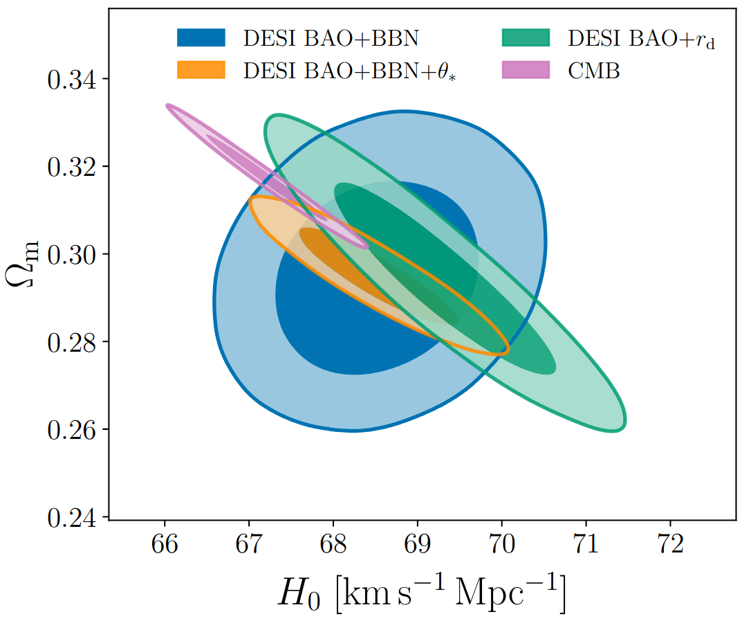
$\Omega := \{ \Omega_m, \Omega_\Lambda, H_0, \sigma_8, f_\mathrm{NL},...\}$

inference

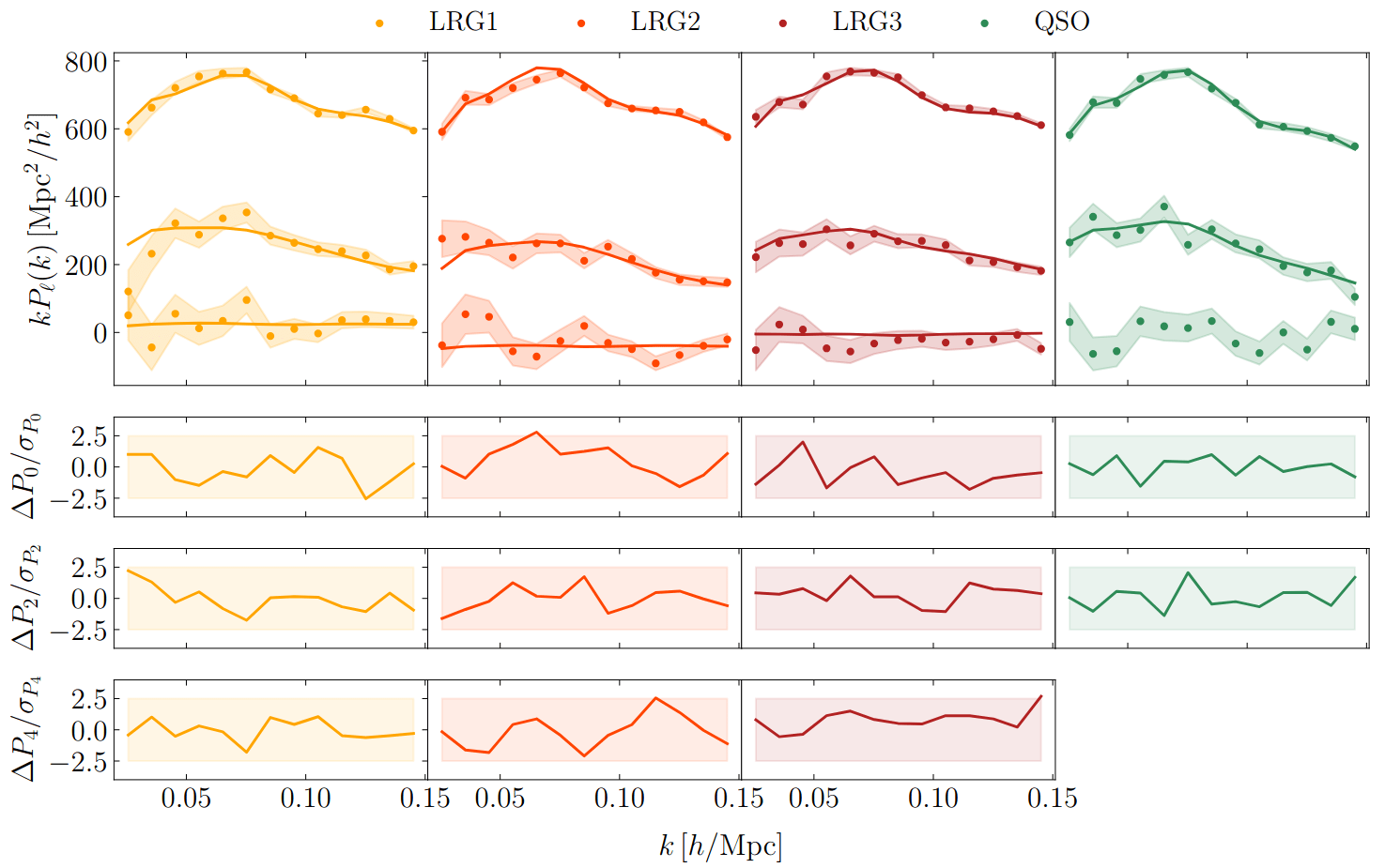
$P$

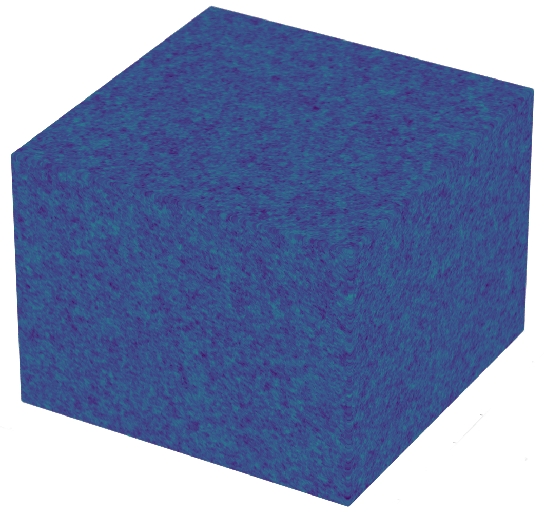
$\Omega$

$\delta_L$

$\delta_g$

Cosmological inference

$\Omega := \{ \Omega_m, \Omega_\Lambda, H_0, \sigma_8, f_\mathrm{NL},...\}$

$\Omega$

$\delta_L$

$\delta_g$

inference

$\delta_L$

$\delta_g$

$\Omega$

Field-level inference

Summary stat inference

$\Omega$

$s$

$\delta_g$

$\Omega$

$\delta_L$

$s$

marginalize

condition

marginalize

$\Omega$

$s$

$\delta_g$

$\Omega$

$\delta_L$

condition

Two approaches to cosmological inference

Cosmo model

$\mathrm{p}(\Omega,s)$

$\mathrm{p}(\Omega \mid s)$

$\Omega$

$\delta_g$

$\mathrm{p}(\Omega,\delta_L,\delta_g, s)= \mathrm{p}(s \mid \delta_g) \, \mathrm{p}(\delta_g \mid \Omega,\delta_L)\, \mathrm{p}(\delta_L \mid \Omega)\, \mathrm{p}(\Omega)$

$\mathrm{p}(\Omega,\delta_L \mid \delta_g)$

$\mathrm{p}(\Omega \mid \delta_g)$

$\delta_g$

$\Omega$

$\delta_L$

$s$

Two approaches to cosmological inference

Cosmo model

Problem:

$s$ is too simple $\implies$ lossy compression
$s$ is too complex $\implies$ intractable marginalization

The Problem:

high-dimensional integral $$\mathrm{p}(\Omega \mid \delta_g) = \int \mathrm{p}(\Omega, \delta_L \mid \delta_g) \;\mathrm d \delta_L$$
To probe scales of $15\ \mathrm{Mpc}/h$ in DESI volume, $\operatorname{dim}(\delta_L) \simeq 1024^3$

The Promise:

"lossless" explicit inference

Nguyen+2024

Field-level inference

Summary stat inference

High-dimensional sampling is hard

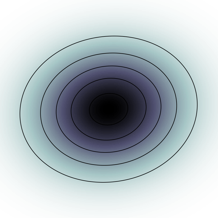
A drunk man will find his way home, but a drunk bird may get lost forever $(\mathrm p\approx 0.66)$

🌸 Shizuo Kakutani

$-\nabla$

$d \approx 1$

🏠

🚶‍♀️

To maintain constant move-away probability, step-size $\simeq d^{-1/2}$

$d \gg 1$

🪺

🐦

Canonical/Microcanonical MCMC samplers

$\mathcal H(\boldsymbol q, \boldsymbol p) = \frac {\boldsymbol p^\top M^{-1} \boldsymbol p} {2 m(\boldsymbol q)} - \frac{m(\boldsymbol q)}{2}, \qquad m:=e^{-U/(d-1)}$
samples microcanonical/isokinetic ensemble $$\mathrm p_\text{MC}(\boldsymbol q, \boldsymbol p) \propto \delta(\mathcal H(\boldsymbol q, \boldsymbol p)) \propto \mathrm p (\boldsymbol q) \delta(\dot{\boldsymbol q}^\top M \dot{\boldsymbol q} - 1)$$

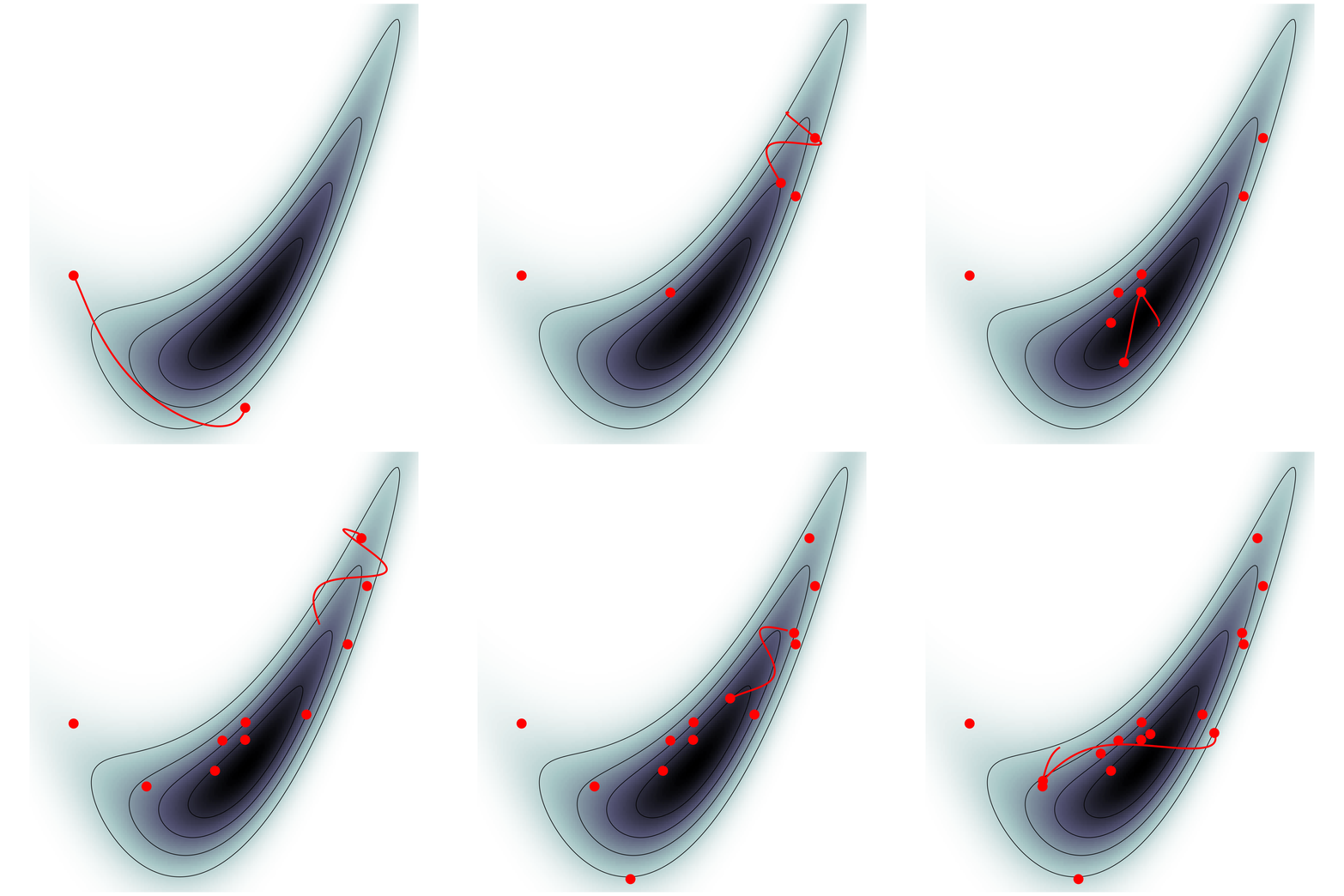
Hamiltonian Monte Carlo (e.g. Neal2011)

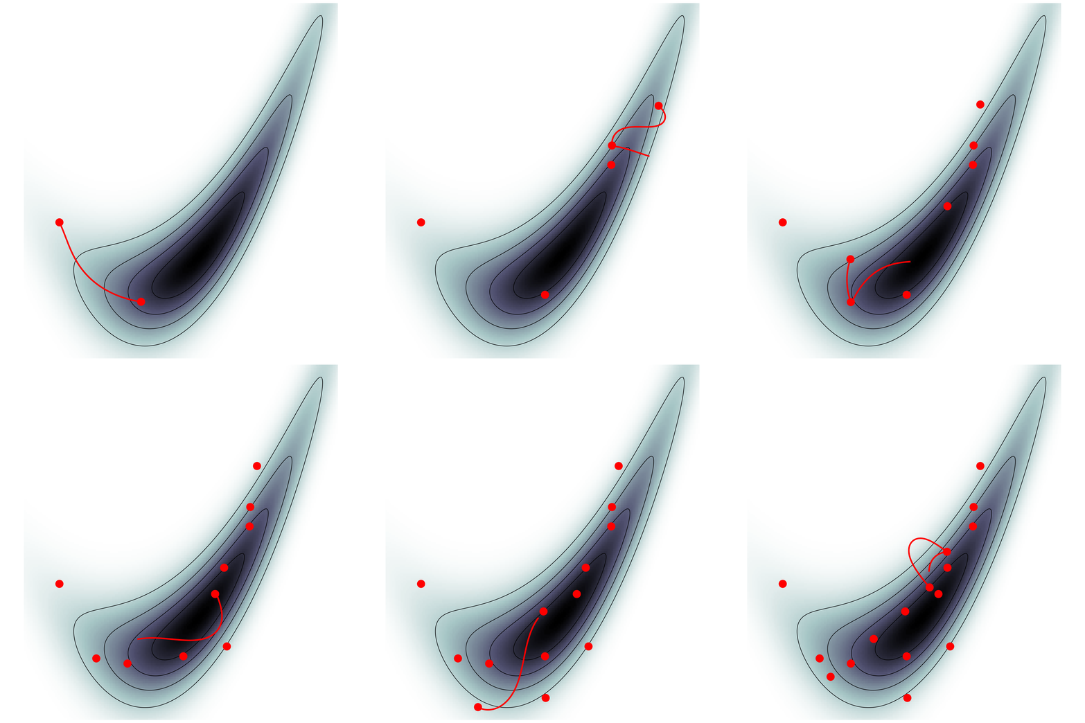
MicroCanonical HMC (Robnik+2022)

$\mathcal H(\boldsymbol q, \boldsymbol p) = U(\boldsymbol q) + \frac 1 2 \boldsymbol p^\top M^{-1} \boldsymbol p$
samples canonical ensemble $$\mathrm p_\text{C}(\boldsymbol q, \boldsymbol p) \propto e^{-\mathcal H(\boldsymbol q, \boldsymbol p)} \propto \mathrm p(\boldsymbol q)\,\mathcal N(\boldsymbol 0, M)$$

Samplers comparison

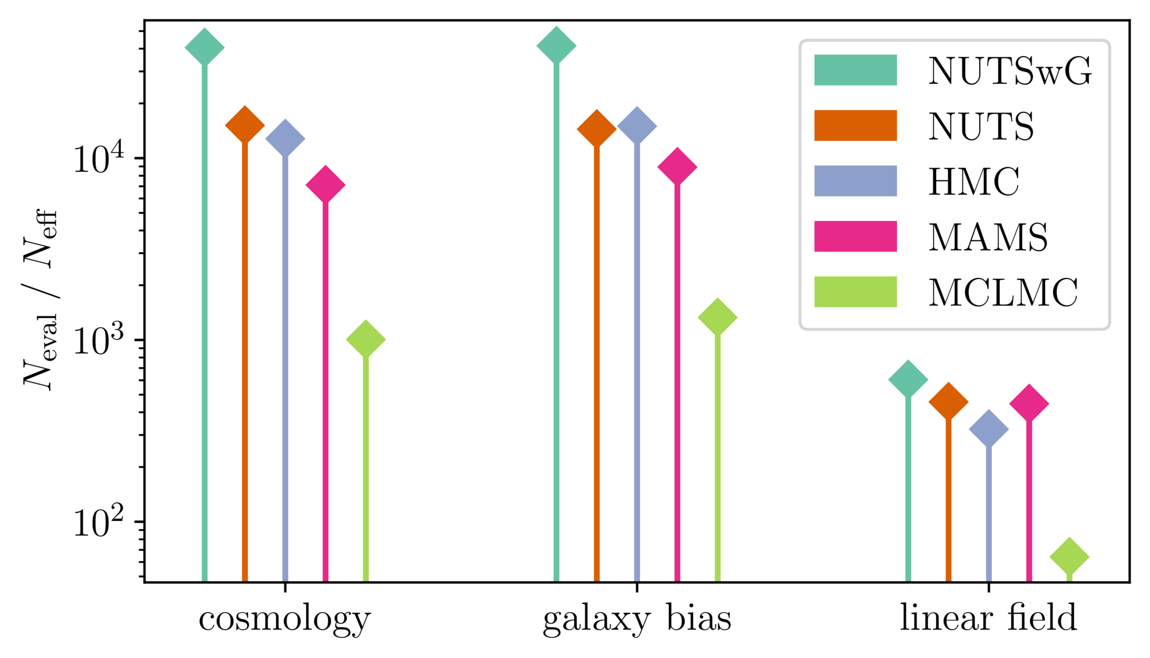
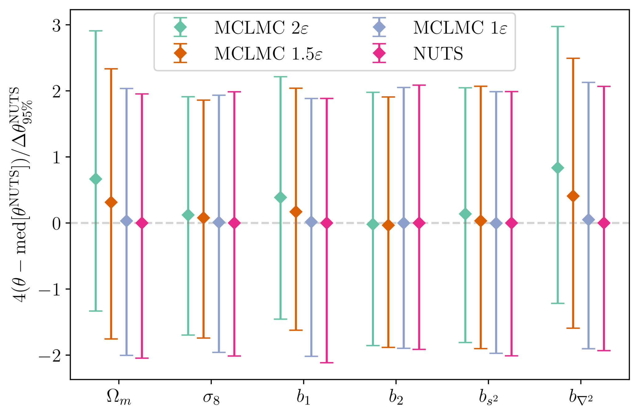
>10 times less evaluations required

Different samplers and strategies used for FLI, additional comparisons required.
Consistent benchmark for field-level from galaxy surveys:
github.com/hsimonfroy/benchmark-field-level

Simon+2025

= NUTS within Gibbs
= auto-tuned HMC

= adjusted MCHMC
= unadjusted Langevin MCHMC

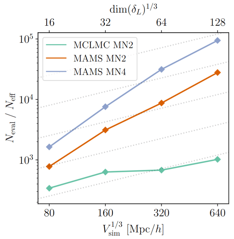
adjusted sampler

unadjusted sampler

= NUTS within Gibbs
= auto-tuned HMC

= adjusted MCHMC
= unadjusted Langevin MCHMC

Benchmark results

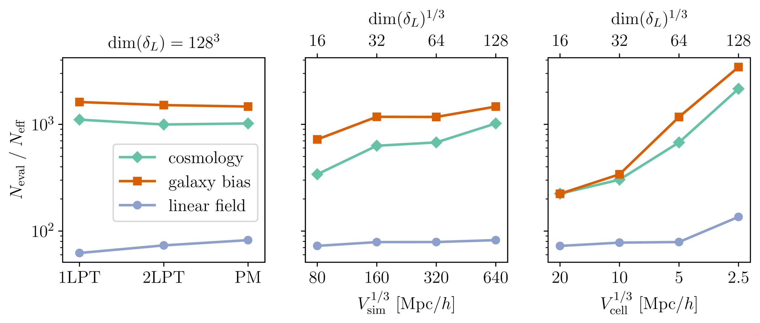
Promising for future inferences, going multi-GPU using JaxDecomp

Mildly dependent with respect to formation model and volume

Probing smaller scales could be harder

MCLMC sampler + field-level preconditioning assuming a linear Kaiser model:
4h on a 8GPU-node for $128^3$ PM inference

At the end of the day

Simon+2025

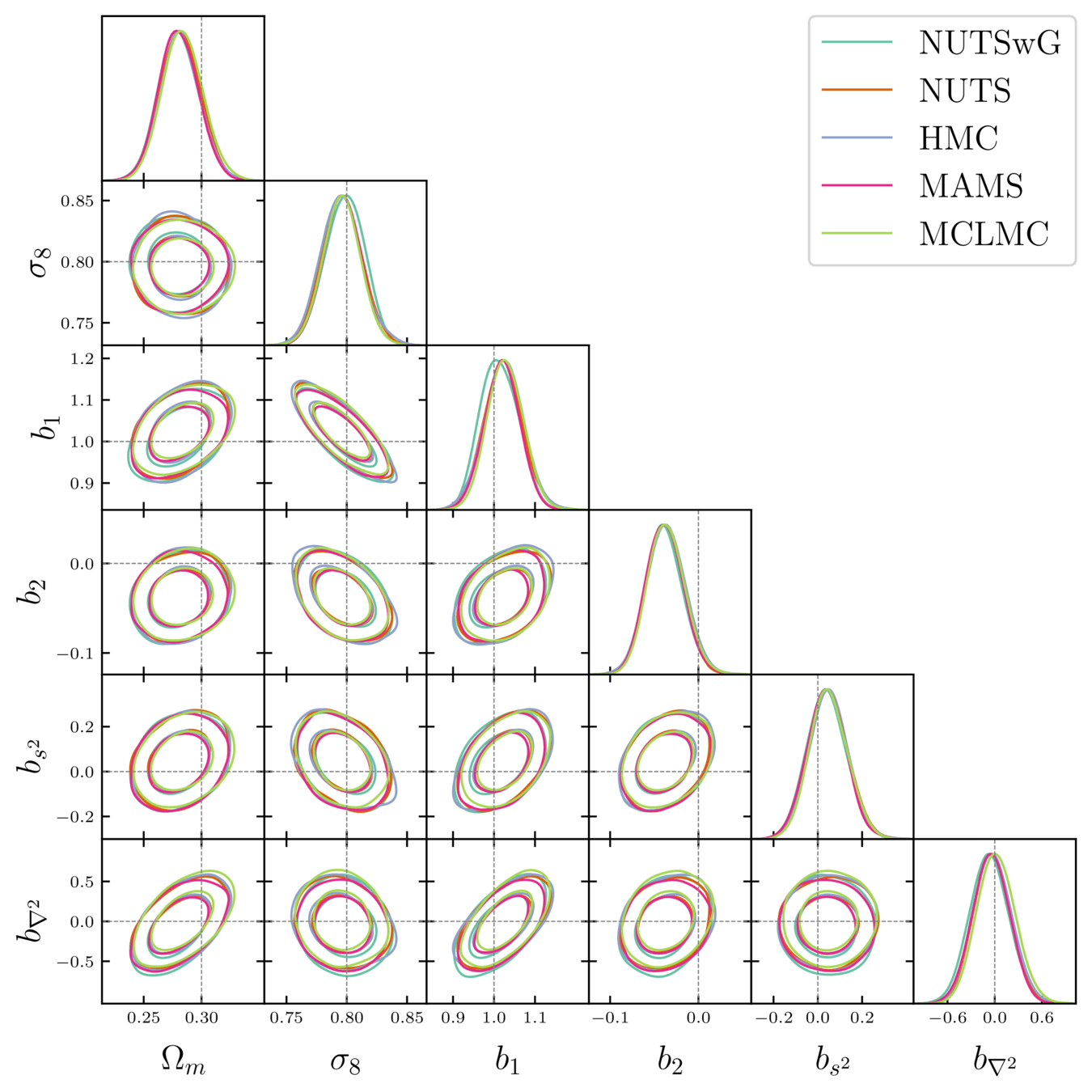
MCLMC + field-level preconditioning:
4h on a GPU-node for $128^3$ PM inference
$\approx 10^5$ simulator calls

Field-Level modeling of PNG

Sample initial conditions, add PNG
$$\phi=\phi_L+{\color{purple}f_{\mathrm{NL}}}\phi_L^{2}$$
Lagrangian bias expansion
$$w_g = \sum_{\mathbb O} b^L_{\mathbb O} [\mathbb O_{L}] \supset {\color{purple}f_{\rm NL} b_\phi}\phi_L + {\color{purple} f_{\rm NL} b_{\phi\delta}} \phi_L \delta_{L}$$
Evolve and weight particles on mesh
Noise + selection
$$n_g \sim \mathcal N({\color{purple}\bar n_g } W(1+\delta_g),\, {\color{purple}\bar n_g }W({\color{purple}s_\varepsilon}+{\color{purple}s_{\varepsilon\delta}}\delta_L))$$

3 main PNG contributions,
2 options:

infer the 3 as independent
assume "mass relations"
$$\begin{align*}b_\phi &=2\delta_c({\color{purple} b_1}+1-p_\phi)\\b_{\phi \delta} &=2 (\delta_c {\color{purple} b_2}+ {\color{purple} b_1})\end{align*}$$(Lagrangian frame)

Fast and differentiable model in

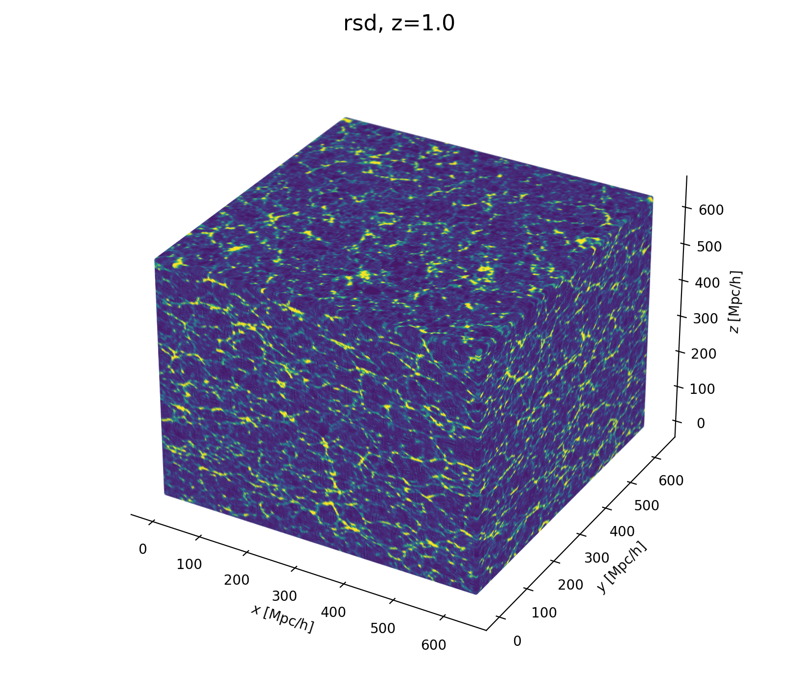
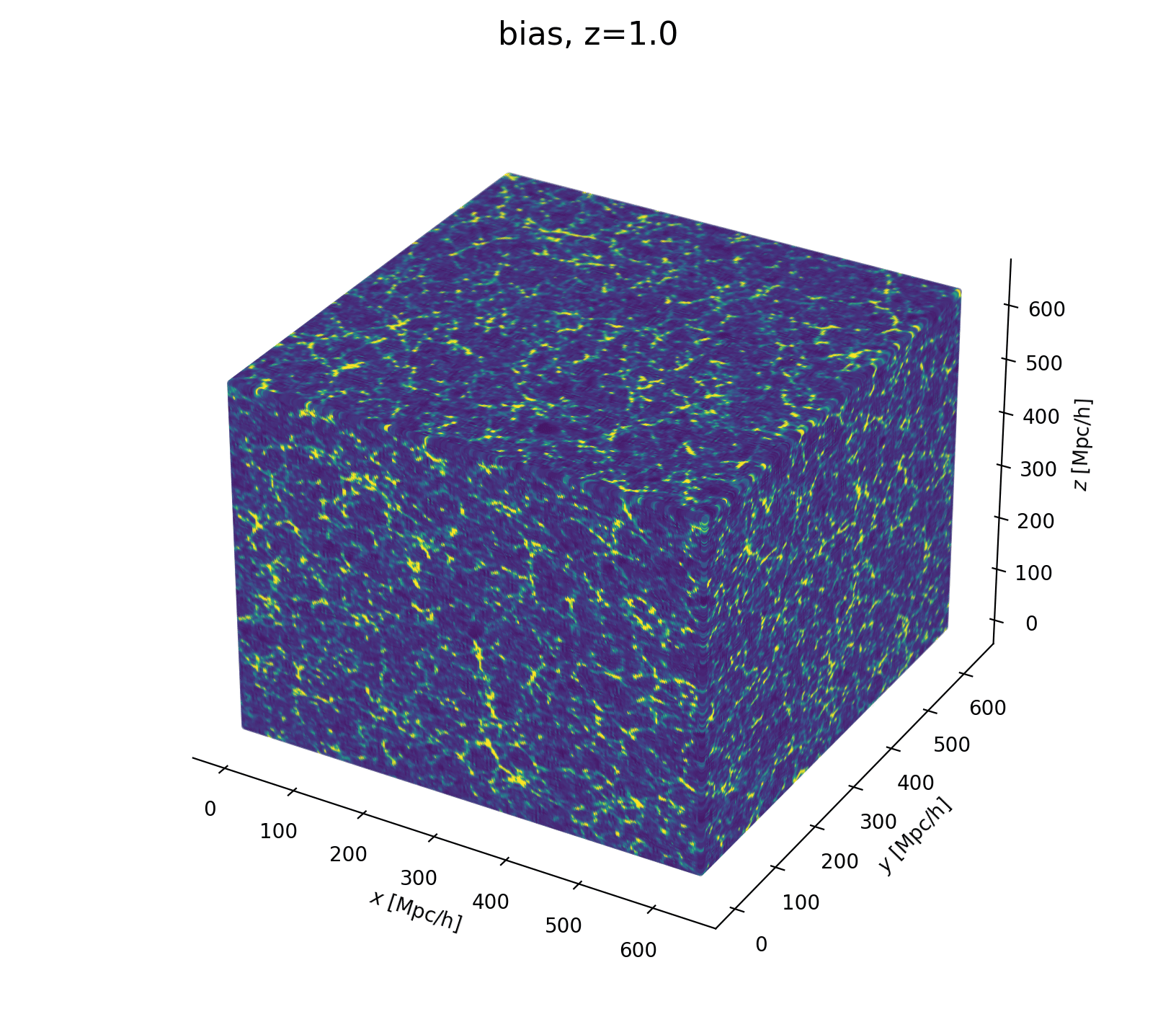
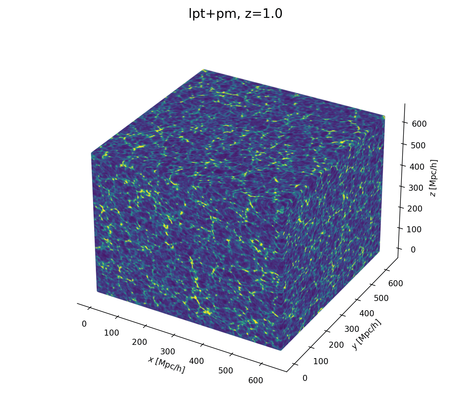
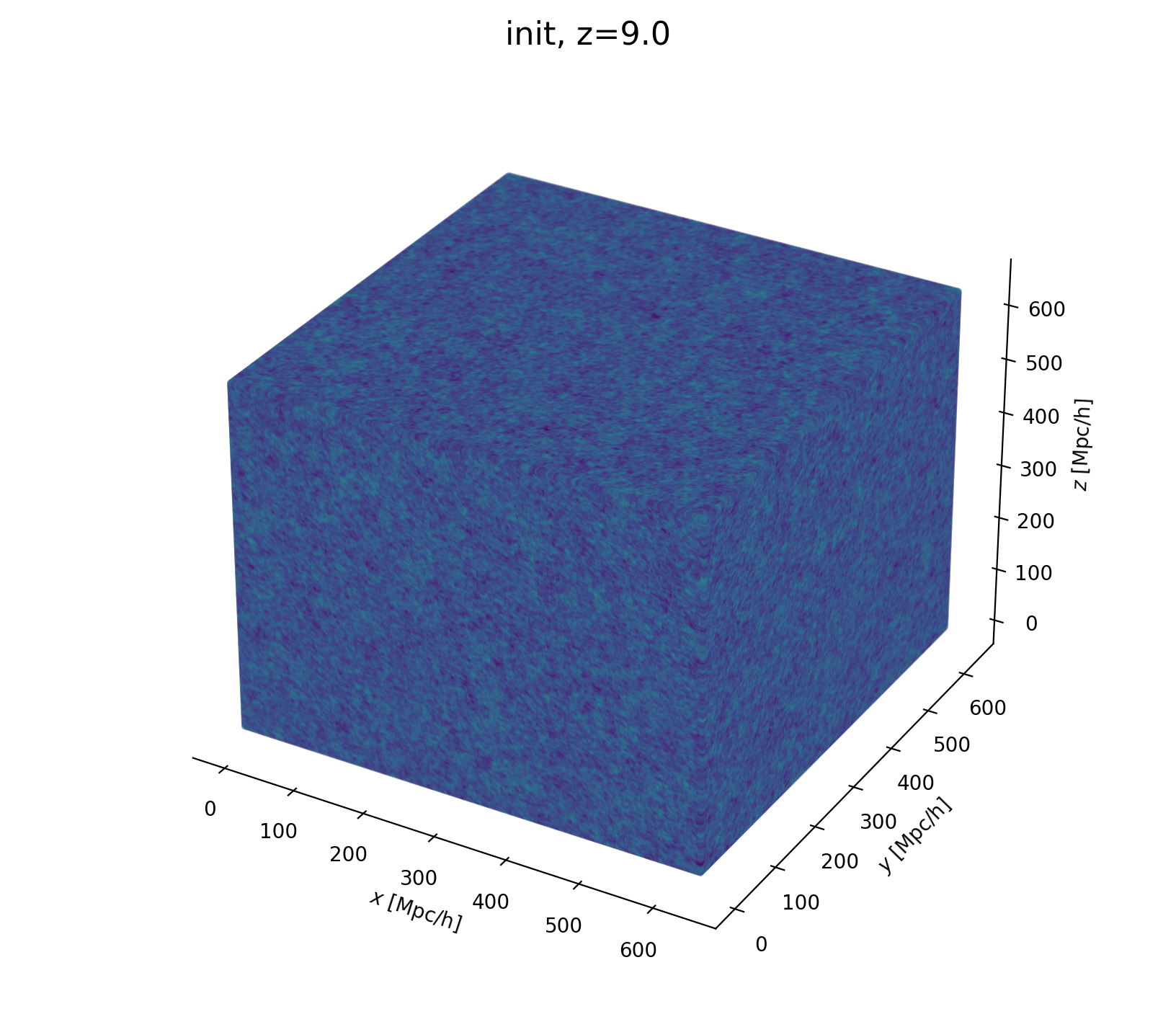
Fast and differentiable model with

Field-Level sampling

Inferring jointly cosmology, bias parameters, and initial conditions allows full universe history reconstruction

+ preconditioning = $128^3$ inference in 2h on a single GPU node (Simon+2025)

+

high-dim MCMC

MCLMC (Robnik+2022)

Field-Level Model

$b$

$\delta_g$

$\Omega$

$\delta_L$

Field-Level Inference of PNG

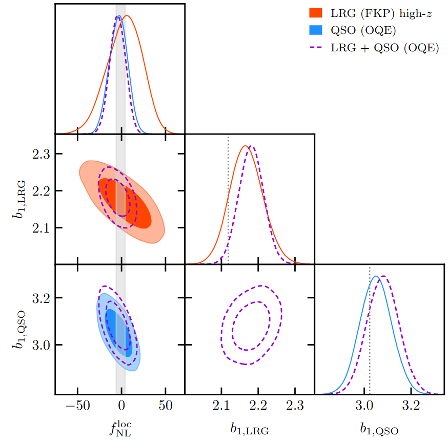
On $(3\ \mathrm{Gpc}/h)^3$ PNGUnitsim-XL

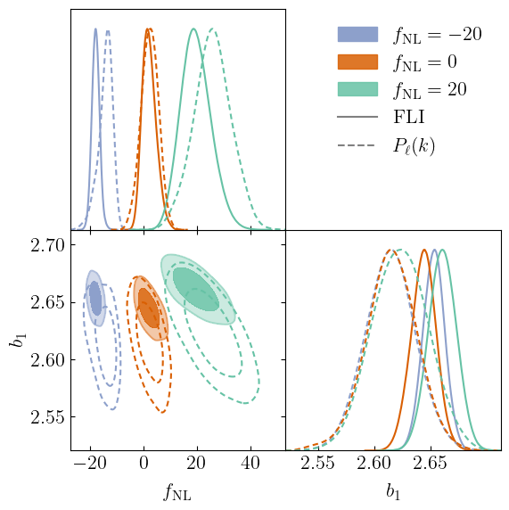
$\textrm{FLI at } k_\mathrm{Nyq} = 0.075\ h/\mathrm{Mpc}\ (64^3)$
$P_{\{0,2\}}(k) \textrm{ at } k_\mathrm{max} = 0.08 h/\mathrm{Mpc}$

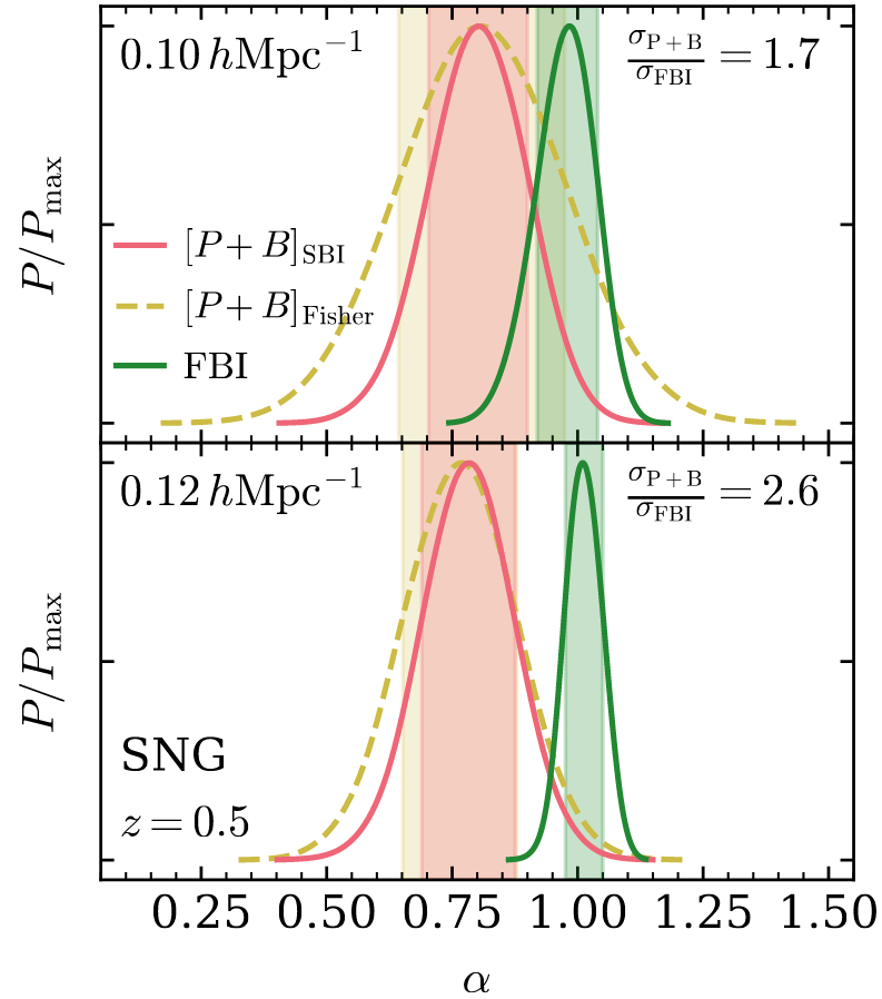
Recovers true $f_\mathrm{NL}$ and fitted $b_1$ assuming fitted $p_\phi$ (see Santiago's)

$$\mathrm{LRG}\, z=0.74$$ 5% to 30% gain

$$\mathrm{QSO}\, z=1.83$$ 20% to 50% gain

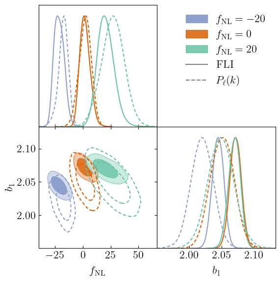
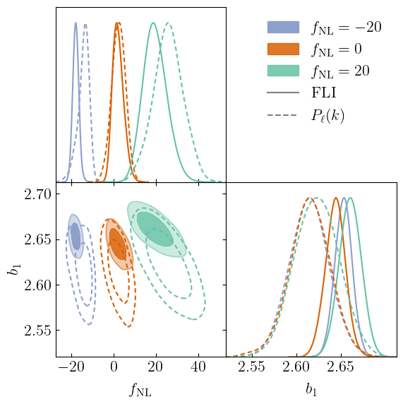
Field-Level Inference of PNG

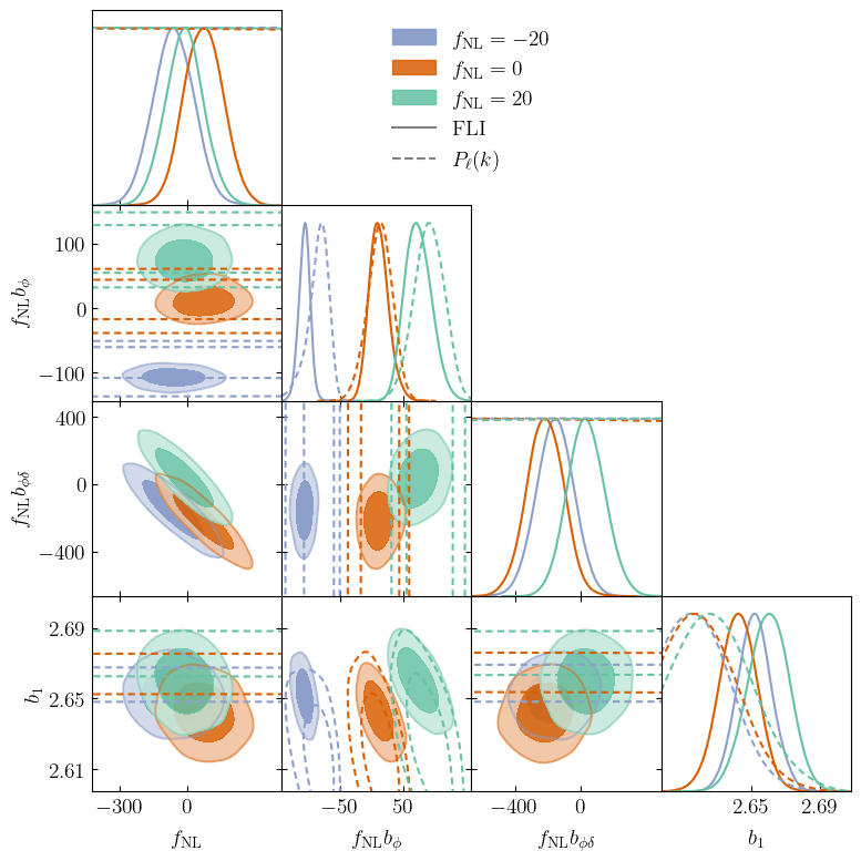
Where does the information come from?

Mass relation with higher $b_1$?
2nd order terms $(f_\mathrm{NL}, f_\mathrm{NL} b_{\phi \delta})$?
$f_\mathrm{NL} b_{\phi}$ from higher $n$-point?

Fit separately and compare:

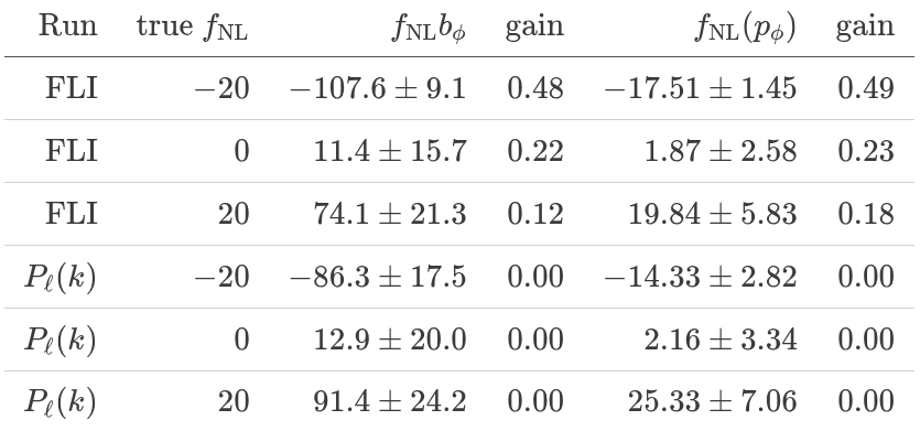
Similar gain on $f_\mathrm{NL} b_\phi$, independent of $b_1$, so probably higher $n$-point $f_\mathrm{NL} b_\phi$ signal
2nd order terms are constrained but does not provide much constraint on $f_\mathrm{NL}$

Toward more survey realism

Next steps:

Cutsky mocks validation
Contaminated mocks validation
Application to DESI LRG and QSO
Multi-probe analyses (see Jonathan's)

$k_\mathrm{Nyq} \approx 0.04\, h/\mathrm{Mpc}$

Example on LRG SGC footprint

Toward more survey realism
on LRG SGC footprint

Ongoing:

Cut-sky validation on PNG-UNITsims, in prep.
Systematics model validation on contaminated mocks
Application to DESI LRG and QSO

$\sigma[f_\mathrm{NL}] \approx 20$, consistent with power spectrum analysis (Chaussidon+2024)

PRELIMINARY

$k_\mathrm{max} \approx 0.04\, h/\mathrm{Mpc}$

Prior on
- Cosmology $\Omega$
- Initial field $\delta_L$
- EFT parameters
  (Dark matter-galaxy connection)
LSS formation: 2LPT or PM
(BullFrog or FastPM)
Apply galaxy bias
Redshift-Space Distortions
Observational noise

Field-Level Modeling

Fast and differentiable model thanks to ($\texttt{NumPyro}$ and $\texttt{JaxPM}$)

Sample initial conditions
LSS formation: 2LPT or N-body PM
(BullFrog or FastPM) lightcone
EFT-based galaxy bias
Redshift-Space Distortions
Observational noise and systematics

Field-Level Modeling and Inference

Fast and differentiable model with

+ field-level preconditioning = $128^3$ PM inference in 4h on a single GPU node

MicroCanonical sampling

+

Simon+2025

Sample initial conditions
LSS formation: 2LPT or N-body PM
(BullFrog or FastPM) lightcone
EFT-based galaxy bias
Redshift-Space Distortions
Observational noise and systematics

Fast and differentiable model with

+ field-level preconditioning = $128^3$ PM inference in 4h on a single GPU node

MicroCanonical sampling

+

Simon+2025

Inferring jointly cosmology and initial field allows 3D universe history reconstruction

Field-Level Modeling and Inference

How to N-body-differentiate?

$(\boldsymbol q, \boldsymbol p)$

$\delta(\boldsymbol x)$

$\delta(\boldsymbol k)$

paint*

read*

fft*

ifft*

fft*

*: differentiable, e.g. with via $\texttt{JaxPM}$, in $\mathcal O(n \log n)$

apply forces
to move particles

solve Vlasov-Poisson
to compute forces

$\begin{cases}\dot {\boldsymbol q} \propto \boldsymbol p\\ \dot{\boldsymbol p} = \boldsymbol f \end{cases}$

$\begin{cases}\nabla^2 \phi \propto \delta\\ \boldsymbol f = -\nabla \phi \end{cases} \implies \boldsymbol f \propto \frac{i\boldsymbol k}{k^2} \delta$

How to N-body-differentiate?

$(\boldsymbol q, \boldsymbol p)$

$\delta(\boldsymbol x)$

$\delta(\boldsymbol k)$

$\rm paint$

$\rm read$

$\rm fft$

$\rm ifft$

*: differentiable, e.g. with via $\texttt{JaxPM}$, in $\mathcal O(n \log n)$

$\rm apply\ forces$
$\rm to\ move\ particles$

$\textrm{solve Vlasov-Poisson to}\\ \mathbf{compute\ forces}$

$\begin{cases}\dot {\boldsymbol q} \propto \boldsymbol p\\ \dot{\boldsymbol p} = \boldsymbol f \end{cases}$

$\begin{cases}\nabla^2 \phi \propto \delta\\ \boldsymbol f = -\nabla \phi \end{cases} \implies \boldsymbol f \propto \frac{i\boldsymbol k}{k^2} \delta$

MCMC sampling

Canonical MCMC samplers

Recipe😋 to sample from $\mathrm p \propto e^{-U}$

take particle with position $\boldsymbol q$, momentum $\boldsymbol p$, mass matrix $M$, and Hamiltonian $$\mathcal H(\boldsymbol q, \boldsymbol p) = U(\boldsymbol q) + \frac 1 2 \boldsymbol p^\top M^{-1} \boldsymbol p$$
follow Hamiltonian dynamics during time $L$
$$\begin{cases} \dot {{\boldsymbol q}} = \partial_{\boldsymbol p}\mathcal H = M^{-1}{{\boldsymbol p}}\\ \dot {{\boldsymbol p}} = -\partial_{\boldsymbol q}\mathcal H = - \nabla U(\boldsymbol q) \end{cases}$$and refresh momentum $\boldsymbol p \sim \mathcal N(\boldsymbol 0,M)$
usually, perform Metropolis adjustment
this samples canonical ensemble $$\mathrm p_\text{C}(\boldsymbol q, \boldsymbol p) \propto e^{-\mathcal H(\boldsymbol q, \boldsymbol p)} \propto \mathrm p(\boldsymbol q)\,\mathcal N(\boldsymbol 0, M)$$

gradient guides particle toward high density sets

scales poorly with dimension

must average over all energy levels

Hamiltonian Monte Carlo (e.g. Neal2011)

Microcanonical MCMC samplers

Recipe😋 to sample from $\mathrm p \propto e^{-U}$

take particle with position $\boldsymbol q$, momentum $\boldsymbol p$, mass matrix $M$, and Hamiltonian $$\mathcal H(\boldsymbol q, \boldsymbol p) = \frac {\boldsymbol p^\top M^{-1} \boldsymbol p} {2 m(\boldsymbol q)} - \frac{m(\boldsymbol q)}{2} \quad ; \quad m=e^{-U/(d-1)}$$
follow Hamiltonian dynamics during time $L$
$$\begin{cases} \dot{\boldsymbol q} = M^{-1/2} \boldsymbol u\\ \dot{\boldsymbol u} = -(I - \boldsymbol u \boldsymbol u^\top) M^{-1/2} \nabla U(\boldsymbol q) / (d-1) \end{cases}$$ and refresh $\boldsymbol u \leftarrow \boldsymbol z/ \lvert \boldsymbol z \rvert \quad ; \quad \boldsymbol z \sim \mathcal N(\boldsymbol 0,I)$
usually, perform Metropolis adjustment
this samples microcanonical/isokinetic ensemble $$\mathrm p_\text{MC}(\boldsymbol q, \boldsymbol u) \propto \delta(H(\boldsymbol q, \boldsymbol u)) \propto \mathrm p (\boldsymbol q) \delta(|\boldsymbol u|^2 - 1)$$

single energy/speed level

let's try avoiding that

gradient guides particle toward high density sets

MicroCanonical HMC (Robnik+2022)

Afraid of unadjusted sampling?

Microcanonical dynamics $\implies$ energy should not vary
Numerical integration yields quantifiable errors that can be linked to bias
see e.g. Robnik+2024
Reducing stepsize rapidly brings bias under Monte Carlo error

Primordial Non-Gaussianity from galaxies

Local-type PNG is constrained by the induced scale-dependent bias

$\phi_{\mathrm{NL}}=\phi+{\color{purple}f_{\mathrm{NL}}}\phi^{2}$

$\delta_g(\boldsymbol k)\simeq\left(b_{1}+ b_\phi {\color{purple}f_\mathrm{NL}}k^{-2} \right) \delta_L(\boldsymbol k)$

$f_{\mathrm{NL}}=-3.6_{-9.1}^{+9.0}$

Chaussidon+2024

Probing inflation with galaxies

Local-type PNG can be constrained by induced scale-dependent bias of galaxies

$\phi_{\mathrm{NL}}=\phi+{\color{purple}f_{\mathrm{NL}}}\phi^{2}$

$\delta_g(\boldsymbol k)\simeq\left(b_{1}+ b_\phi {\color{purple}f_\mathrm{NL}}k^{-2} \right) \delta_L(\boldsymbol k)$

$f_{\mathrm{NL}}=-3.6_{-9.1}^{+9.0}$

Chaussidon+2024

Ideal first demonstration for FLI

Most of signal from easier large scales
Result very sensitive to systematics, more directly implemented at field-level
Bonus: fully explicit/explainable, no black box modeling
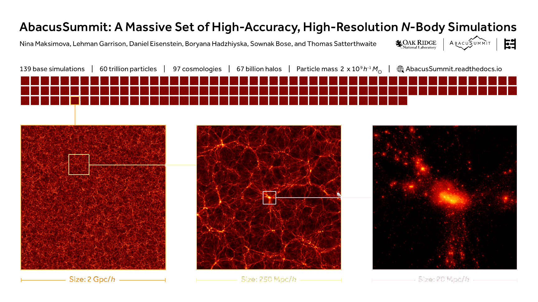
Validate on DESI reference simulations:
- N-body+HOD AbacusSummit
- PNG-UNITsims, largest PNG sims

Field-Level modeling of PNG

Sample initial conditions, add PNG
$$\phi=\phi_L+{\color{purple}f_{\mathrm{NL}}}\phi_L^{2}$$
Lagrangian bias expansion $$\mathcal w_g = \sum_{\mathbb O} b^{\rm L}_{\mathbb O} [\mathbb O_{\rm L}] \supset {\color{purple}f_{\rm NL} b_\phi}\phi_{\rm L} + {\color{purple} f_{\rm NL} b_{\phi\delta}} \phi_{\rm L} \delta_{\rm L}$$
$$w_g = \sum_{\mathbb O} b^L_{\mathbb O} [\mathbb O_{L}] \supset {\color{purple}f_{\rm NL} b_\phi}\phi_L + {\color{purple} f_{\rm NL} b_{\phi\delta}} \phi_L \delta_{L}$$
Evolve and weight particles on grid
Noise + selection
$$n_g \sim \mathcal N(W{\color{purple} \bar n_g} (1+\delta_g),\, W{\color{purple}\bar n_g \sigma_0}(1+{\color{purple}\sigma_\delta}\delta_g))$$

3 main PNG parameters, 2 options:

infer the 3 as independent
assume "universality" relations
$$\begin{align*}b_\phi &=2\delta_c({\color{purple} b_1}+1-p_\phi)\\b_{\phi \delta} &=2 (\delta_c {\color{purple} b_2}+ {\color{purple} b_1})\end{align*}$$(Lagrangian form)

Fast and differentiable model in

Field-Level modeling of PNG

Sample initial conditions, add PNG
$$\phi_{\mathrm{NL}}=\phi+{\color{purple}f_{\mathrm{NL}}}\phi^{2}$$
Lagrangian bias of particles at $\boldsymbol q^\mathrm{in}$ $$\mathcal O_{\rm L}=1+{\color{purple}b_{1}}\,\delta_{\rm L}+{\color{purple}b_{2}}\delta_{\rm L}^{2}+{\color{purple}b_{s^2}}s^{2}+ {\color{purple}b_{\nabla^2}} \nabla^2 \delta _{\rm L}\\\!\!\!\!\!\!\! + {\color{purple}f_{\rm NL} b_\phi}\phi + {\color{purple} f_{\rm NL} b_{\phi\delta}} \phi \delta_{\rm L}$$
Displace to $\boldsymbol q^\mathrm{fin}$
$\boldsymbol q^\mathrm{fin} = \boldsymbol q^\mathrm{2LPT} + H^{-1}\dot {\boldsymbol q}^\mathrm{2LPT}_\parallel + {\color{purple}b_{\nabla_\parallel}} \nabla_\parallel \delta_\mathrm{L}(\boldsymbol q^\mathrm{in})$
Paint particles on grid
$$(1+\delta_g)(\boldsymbol x) = \int K(\boldsymbol x - \boldsymbol q^\mathrm{fin}) \mathcal O_L(\boldsymbol q^\mathrm{in})\, \mathrm d \boldsymbol q^\mathrm{in}$$
Noise via galaxy stochasticity
$$n_g \sim \mathcal N({\color{purple} \bar n_g} (1+\delta_g),\, {\color{purple}\bar n_g \sigma_0}(1+{\color{purple}\sigma_\delta}\delta_g))$$

3 PNG parameters, 2 options:

infer the 3 as independent
assume "universality" relations
$$\begin{align*}b_\phi &=2\delta_c({\color{purple} b_1}+1-p)\\b_{\phi \delta} &=2 (\delta_c {\color{purple} b_2}+ {\color{purple} b_1})\end{align*}$$(Lagrangian form)

Fast and differentiable model with

Sample initial conditions, add PNG
$$\phi_{\mathrm{NL}}=\phi+{\color{purple}f_{\mathrm{NL}}}\phi^{2}$$
Lagrangian bias of particles at $\boldsymbol q^\mathrm{in}$ $$\mathcal O_{\rm L}=1+{\color{purple}b_{1}}\delta_{\rm L}+{\color{purple}b_{2}}\delta_{\rm L}^{2}+{\color{purple}b_{s^2}}s^{2}+ {\color{purple}b_{\nabla^2}} \nabla^2 \delta _{\rm L}\\\!\!\!\!\!\!\! + {\color{purple}f_{\rm NL} b_\phi}\phi + {\color{purple} f_{\rm NL} b_{\phi\delta}} \phi \delta_{\rm L}$$
Displace to $\boldsymbol q^\mathrm{fin}$
$\boldsymbol q^\mathrm{fin} = \boldsymbol q^\mathrm{disp} + H^{-1}\dot {\boldsymbol q}^\mathrm{disp}_\parallel + {\color{purple}b_{\nabla_\parallel}} \nabla_\parallel \delta_\mathrm{L}(\boldsymbol q^\mathrm{in})$
Paint particles on grid
$$(1+\delta_g)(\boldsymbol x) = \int K(\boldsymbol x - \boldsymbol q^\mathrm{fin}) \mathcal O_L(\boldsymbol q^\mathrm{in})\, \mathrm d \boldsymbol q^\mathrm{in}$$
Noise via galaxy stochasticity
$$n_g \sim \mathcal N({\color{purple} \bar n_g} (1+\delta_g),\, {\color{purple}\bar n_g \sigma_0}(1+{\color{purple}\sigma_\delta}\delta_g))$$

Fast and differentiable model with

$k_\mathrm{evolve}$
(LPT, bias)

$k_\mathrm{paint}$

$k_\mathrm{final}$

$k_\mathrm{init}$

Field-Level modeling of PNG

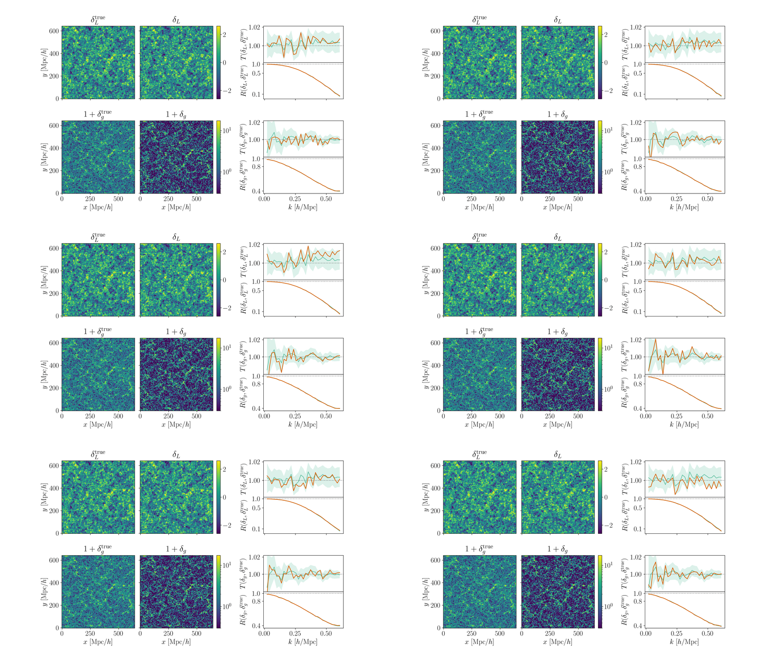
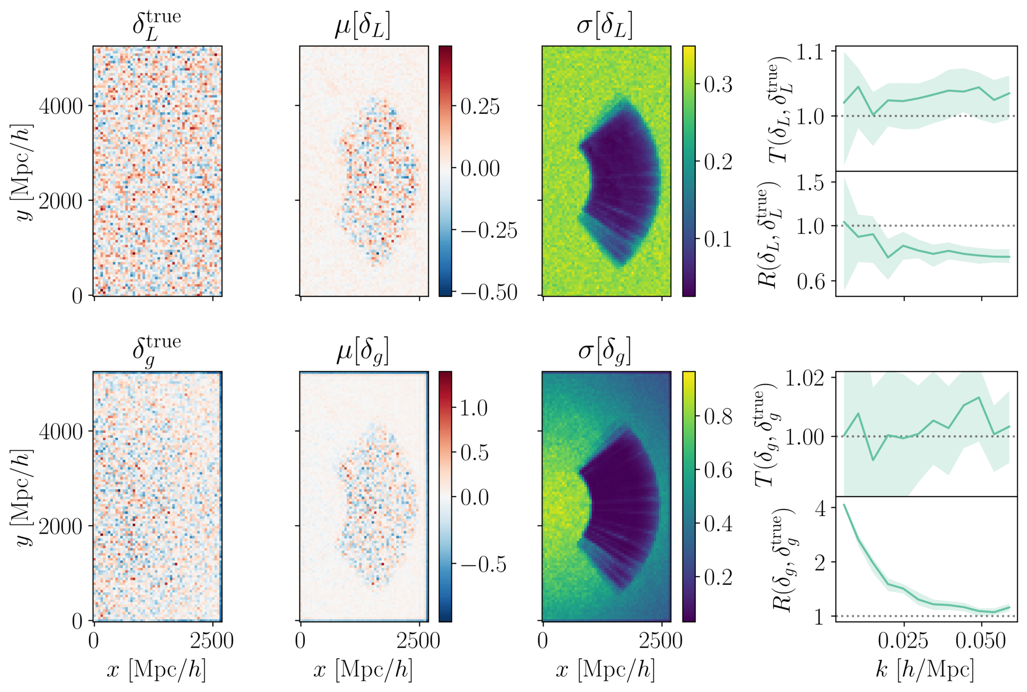
Fitting AbacusSummit+HOD

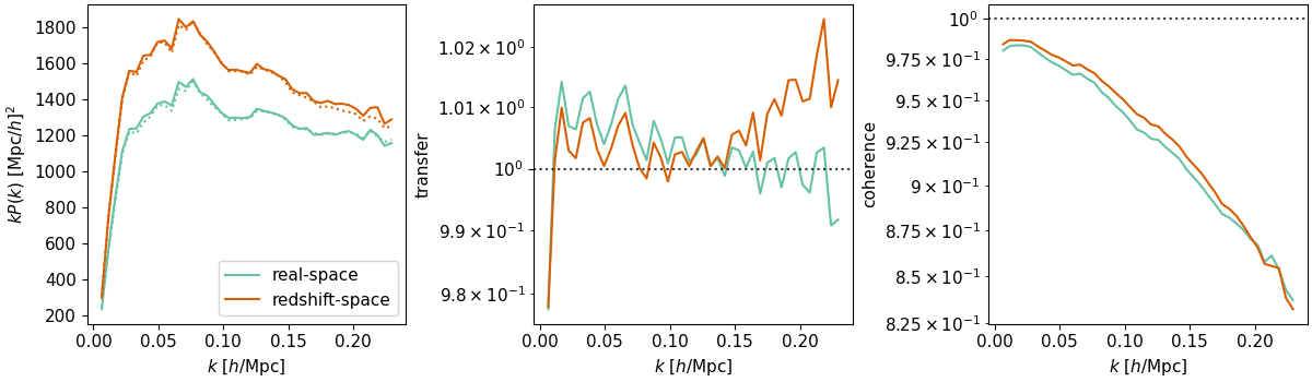
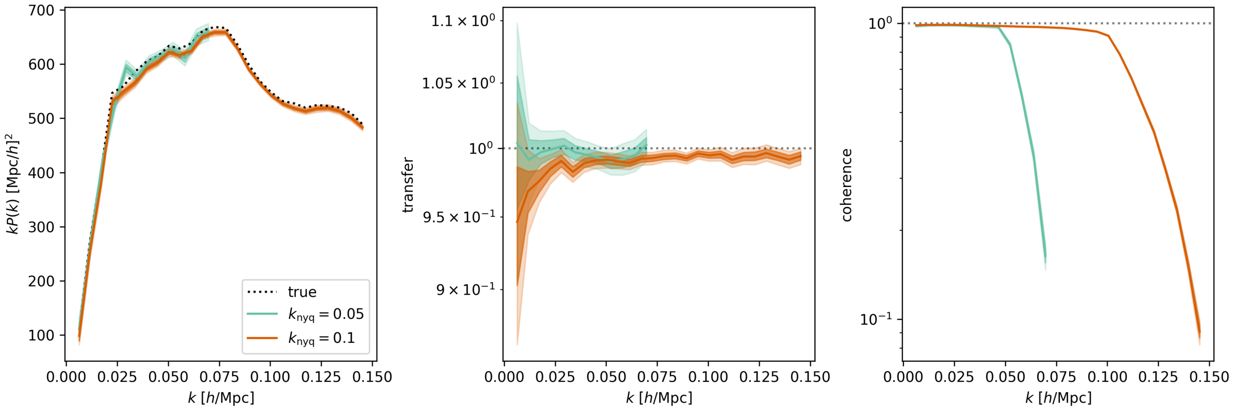
Matter: fix initial conditions. Match within $0.5\%$ at field-level for $k_\mathrm{nyq} < 0.1 h/\mathrm{Mpc} $

Tracer (LRG, $z=0.8$): fix initial conditions and optimize on EFT parameters

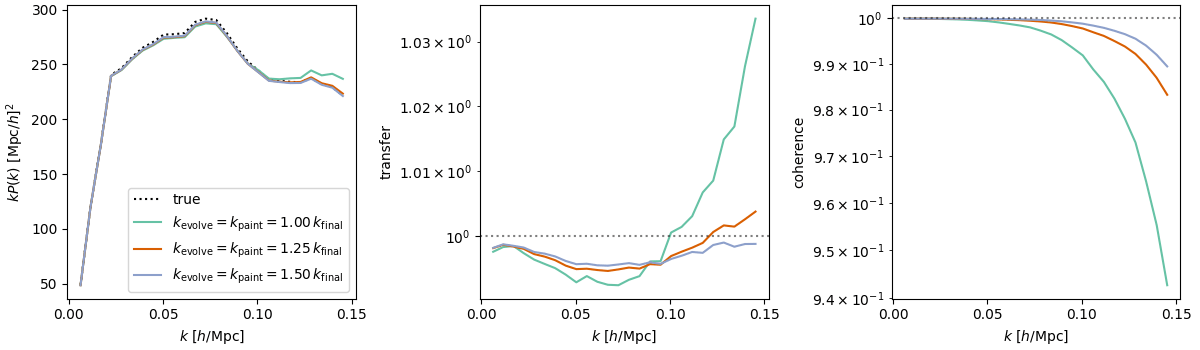
$$\sqrt{P_{\delta} / P_{\delta^\mathrm{true}}}$$ = amplitude info

$$P_{\delta,\delta^\mathrm{true}} / \sqrt{P_{\delta}P_{\delta^\mathrm{true}}}$$ = phase info

Galaxy stochasticity

${\color{purple}\sigma_0}|1+{\color{purple}\sigma_\delta}\delta_g^\mathrm{det}|$
Poisson $\simeq \sigma_0=\sigma_\delta=1$, but fits show sub-Poisson

$k_\mathrm{nyq} \leq 0.15 h/ \mathrm{Mpc}$
$\delta_g \sim \mathcal N(\delta_g^\mathrm{det},\, {\color{purple}❓})$

${\color{purple}\sigma_0}(1+{\color{purple}\sigma_{2}}k^2 + {\color{purple}\sigma_{\mu,2}}(\mu k)^2)$
Negligible for currently probed scales.

Galaxy stochasticity = $\delta_g^\mathrm{true} -\delta_g^\mathrm{det}$, and we take $\delta_g^\mathrm{det}$ to be EFT best fit.

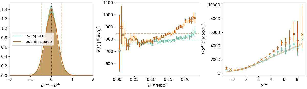
$\sigma^2(\delta^\mathrm{det})$

Preliminary FLI results on PNG

On AbacusSummit + HOD mock ($f_\mathrm{NL}= 0$)

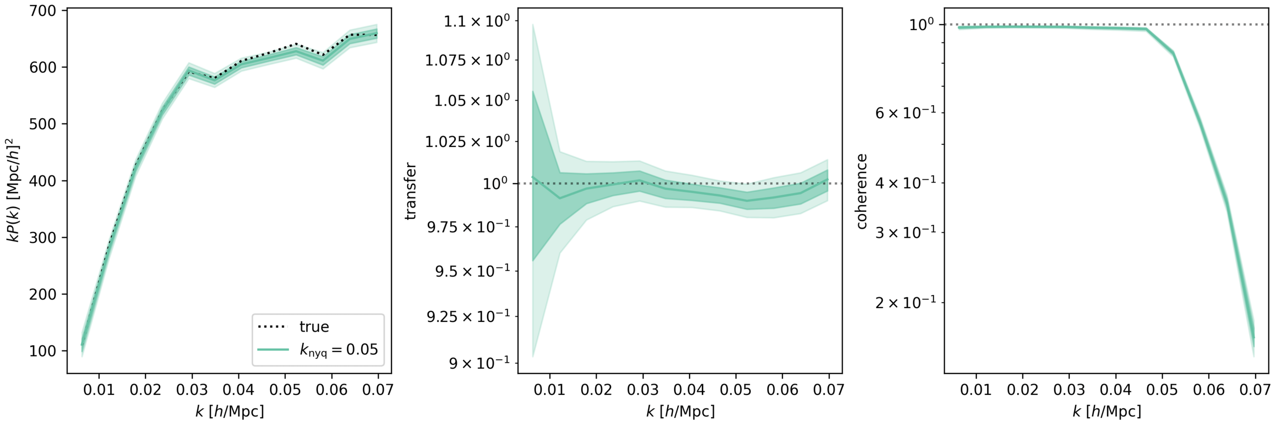
For $k_\mathrm{nyq} = 0.1\ h/\mathrm{Mpc}$,
$f_\mathrm{NL} b_\phi$ compatible, but not $f_\mathrm{NL} b_{\phi \delta}$ nor $f_\mathrm{NL}$

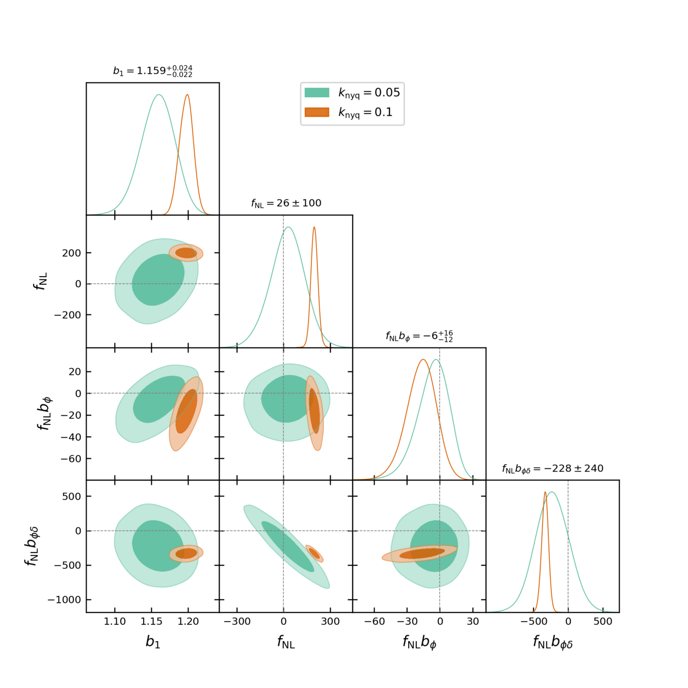
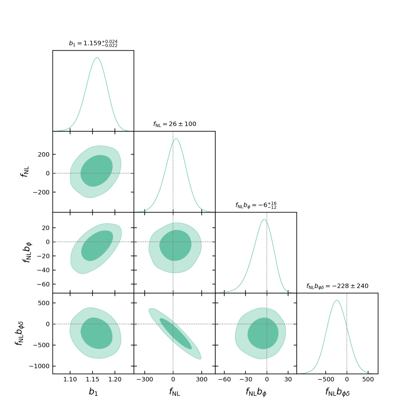
For $k_\mathrm{nyq} = 0.05\ h/\mathrm{Mpc}$, inference compatible with $f_\mathrm{NL}= 0$.
TBD: posterior calibration tests

$(2\ \mathrm{Gpc}/h)^3,\, \mathrm{LRG}\, z=0.8$

PRELIMINARY

Preliminary FLI results on PNG

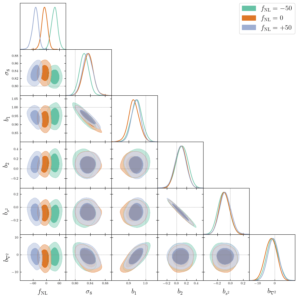
On $f_\mathrm{NL}\neq 0$ FastPM + HOD mocks

Next steps:

confirm the calibration at relevant scales on simulations
Light-cone, survey selection, imaging...
validation on contaminated mocks
Application to DESI LRGs and QSOs

PRELIMINARY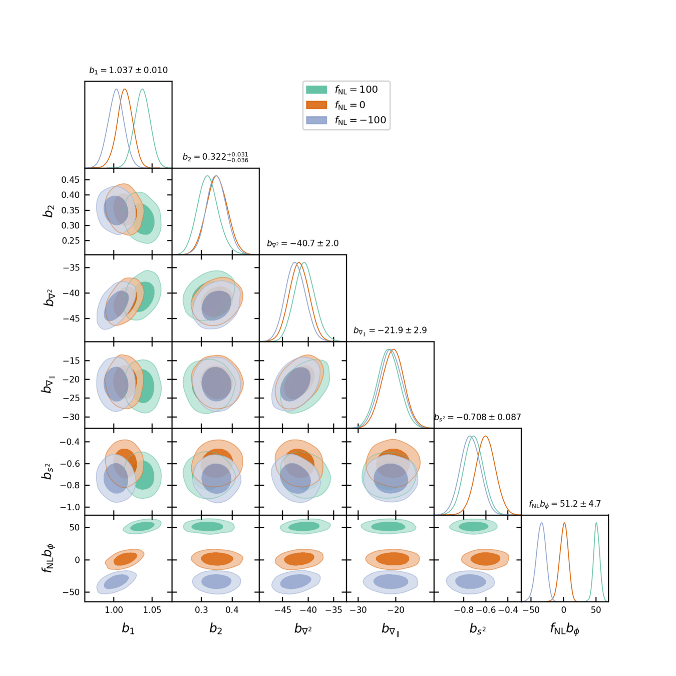

$(2.76\ \mathrm{Gpc}/h)^3,\,k_\mathrm{nyq} = 0.073 h/ \mathrm{Mpc},\\ \mathrm{QSO}\, z=1,\, \operatorname{dim}(\delta_L) = 96^3$

Probing inflation with FLI

NOW: validation on AbacusSummit (DESI reference sims) and FastPM + HOD mocks

$(2.76\ \mathrm{Gpc}/h)^3,\,k_\mathrm{nyq} = 0.073 h/ \mathrm{Mpc},\\ \mathrm{QSO}\, z=1,\, \operatorname{dim}(\delta_L) = 96^3$

PNG, ideal first demonstration of FLI:

Most of signal from easier large scales
Result very sensitive to systematics, more directly implemented at field-level
Bonus: fully explicit/explainable

PRELIMINARY

Next steps:

Validation of survey realism on contaminated mocks
Application to DESI LRGs and QSOs

In prep: Simon+2025

Preliminary FLI results on PNG

On $f_\mathrm{NL}\neq 0$ FastPM + HOD mocks (courtesy of Edmond)

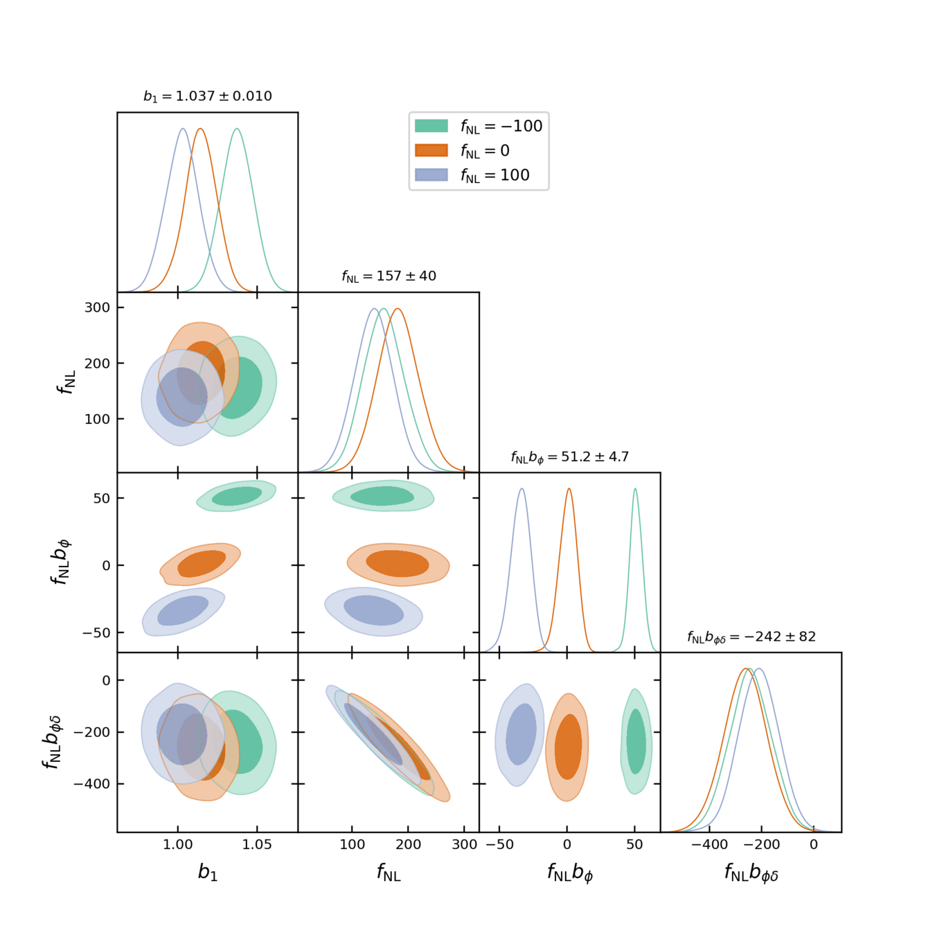
PRELIMINARY

$(2.76\ \mathrm{Gpc}/h)^3,\,k_\mathrm{nyq} = 0.073 h/ \mathrm{Mpc},\\ \mathrm{QSO}\, z=1,\, \operatorname{dim}(\delta_L) = 96^3$

PRELIMINARY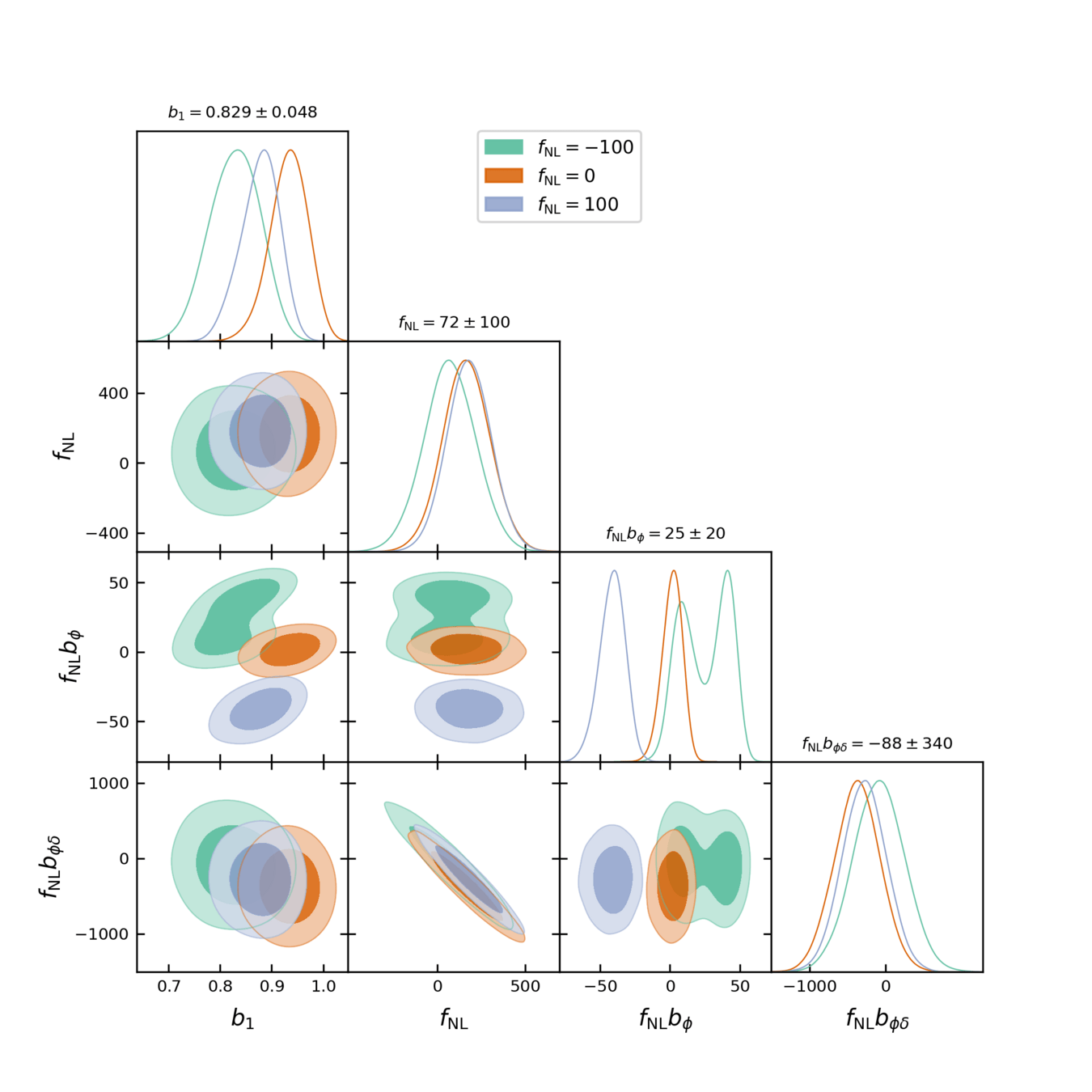

$(2.76\ \mathrm{Gpc}/h)^3,\,k_\mathrm{nyq} = 0.036 h/ \mathrm{Mpc},\\\, \mathrm{QSO}\, z=1,\,\operatorname{dim}(\delta_L) = 48^3$

Next steps:

confirm the calibration at relevant scales on PNG-Unitsims
light-cone, survey selection, imaging...

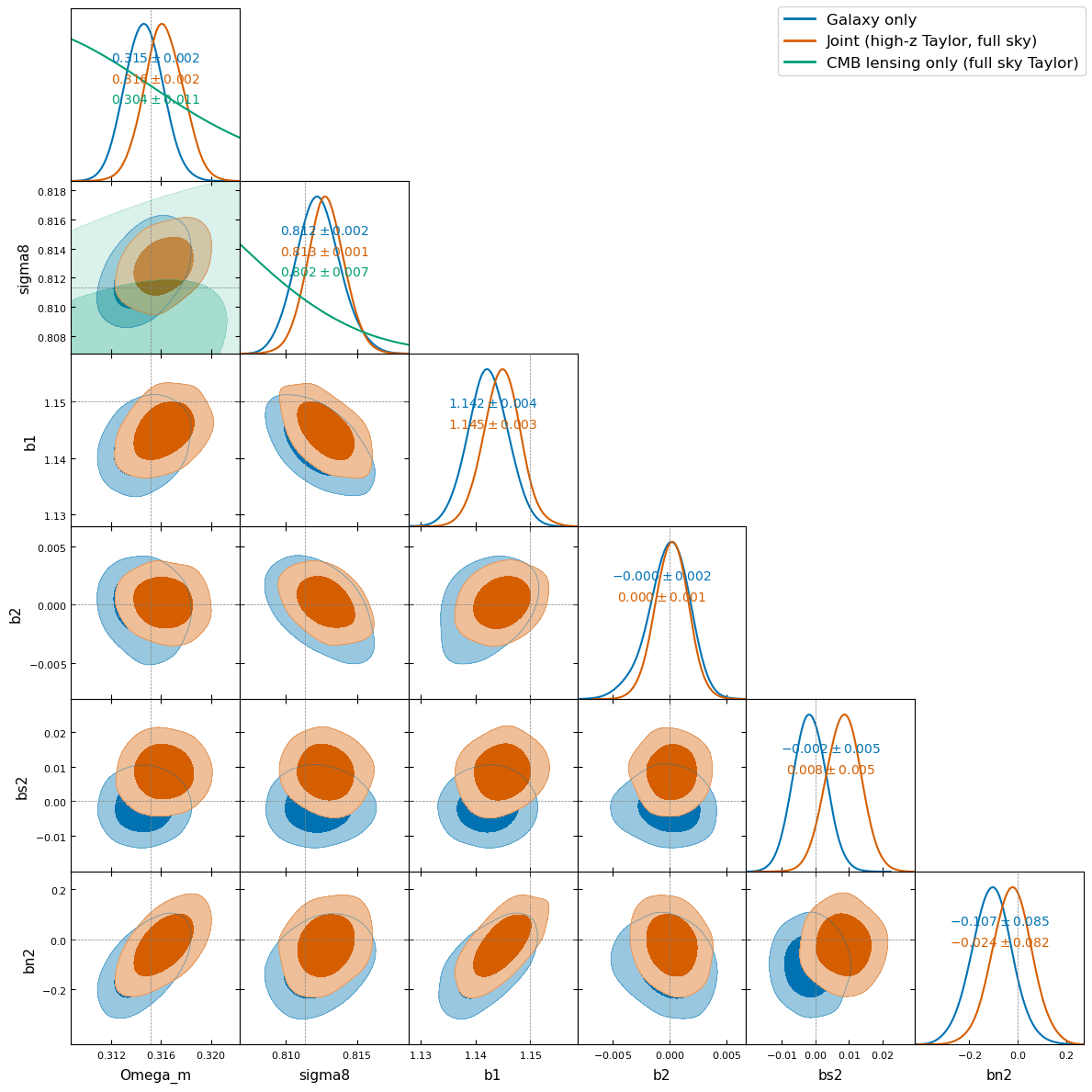
Field-Level Multi-Probing

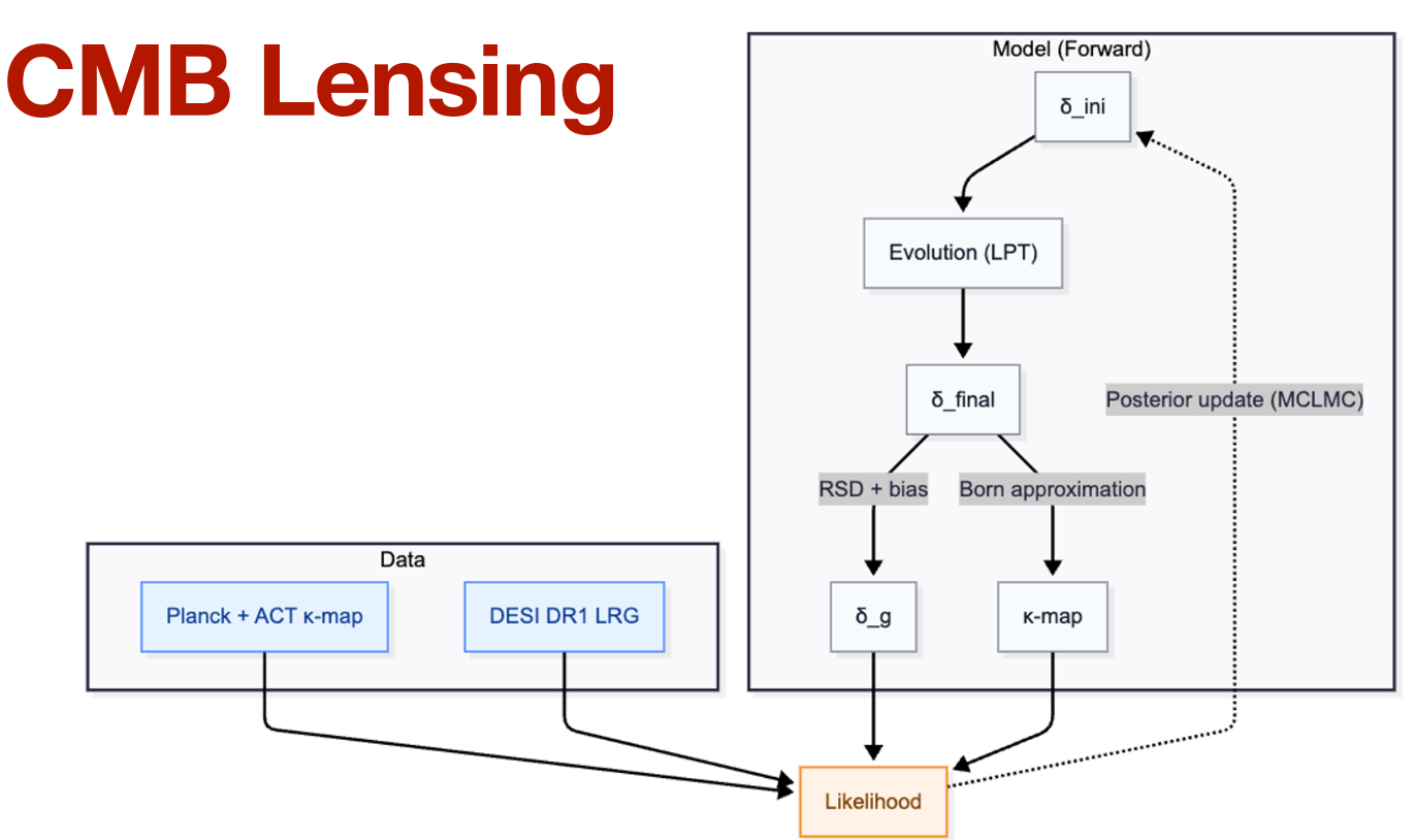
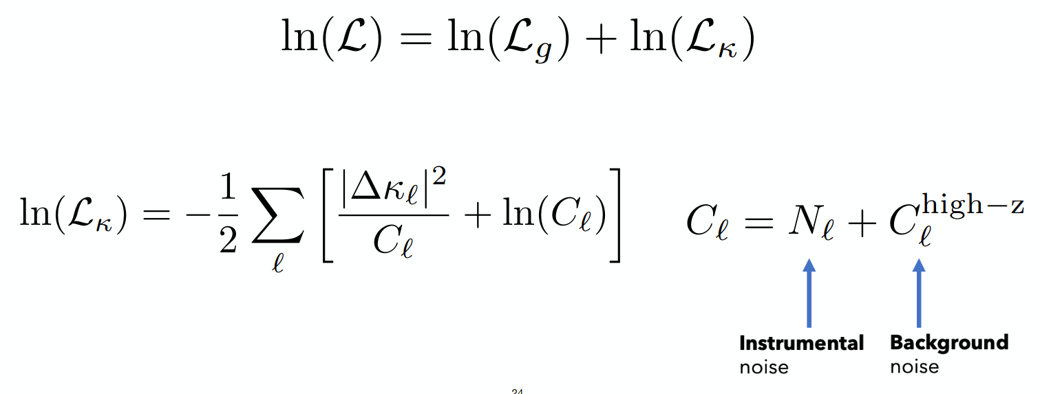
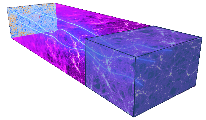
Extend the current galaxy 3D-field pipeline with CMB lensing convergence 2D-field
Joint modeling: cross-correlations are automatically taken into account
Again, fast and differentiable

Jonathan Hawla

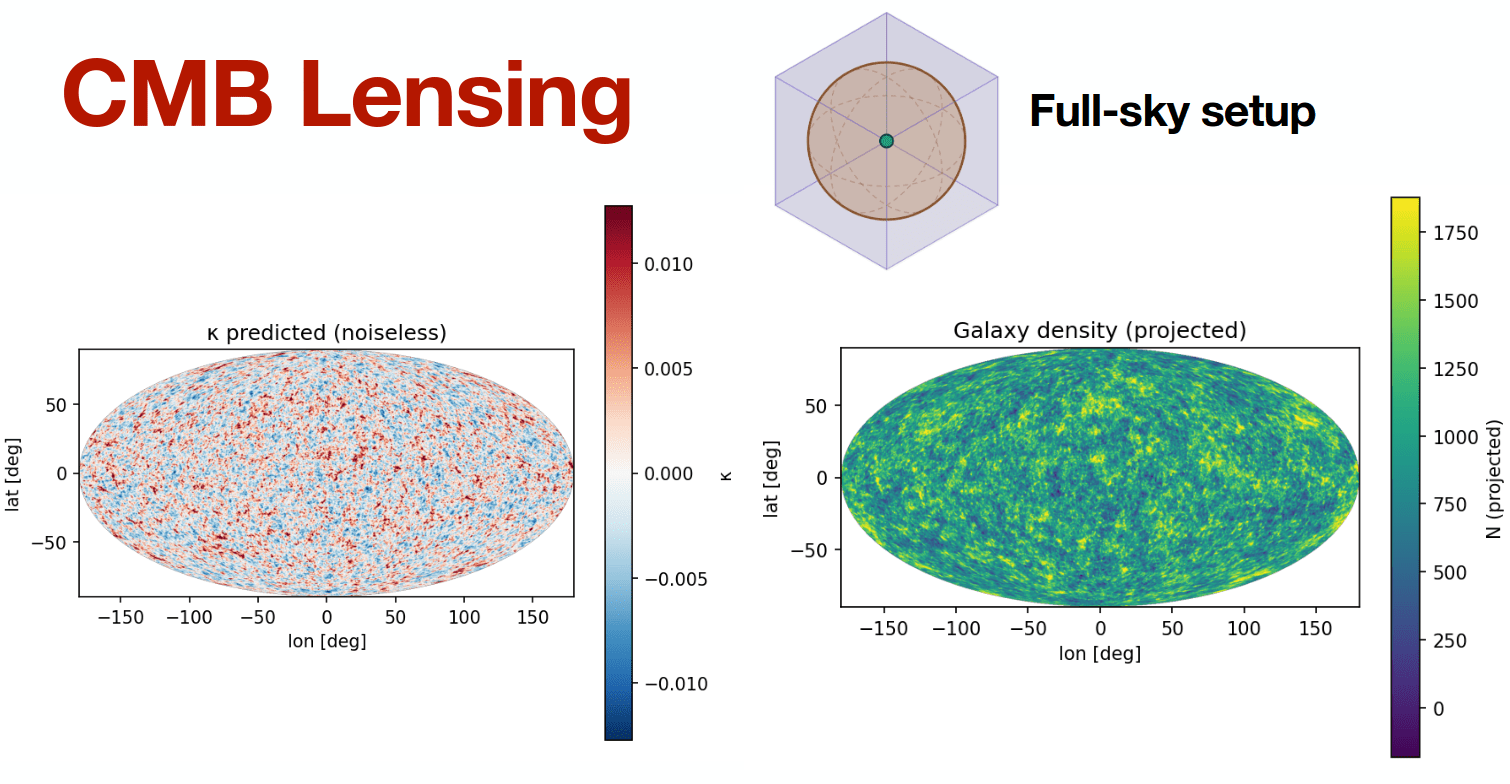
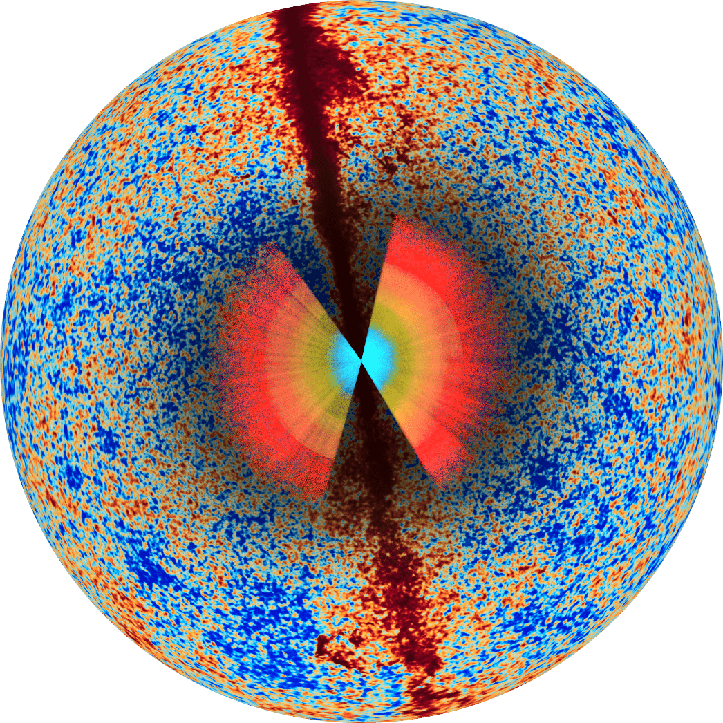
Should we add a $\kappa$ back-screen?
Actually we can analytically marginalize between $z_\mathrm{max}$ and $z_*$

Think (of the CMB) outside the box

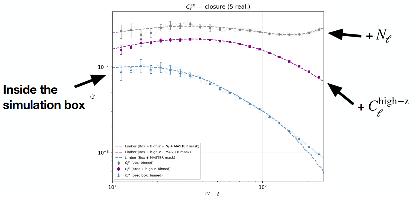
wasted simulated volume

DESI tracers

Ongoing:

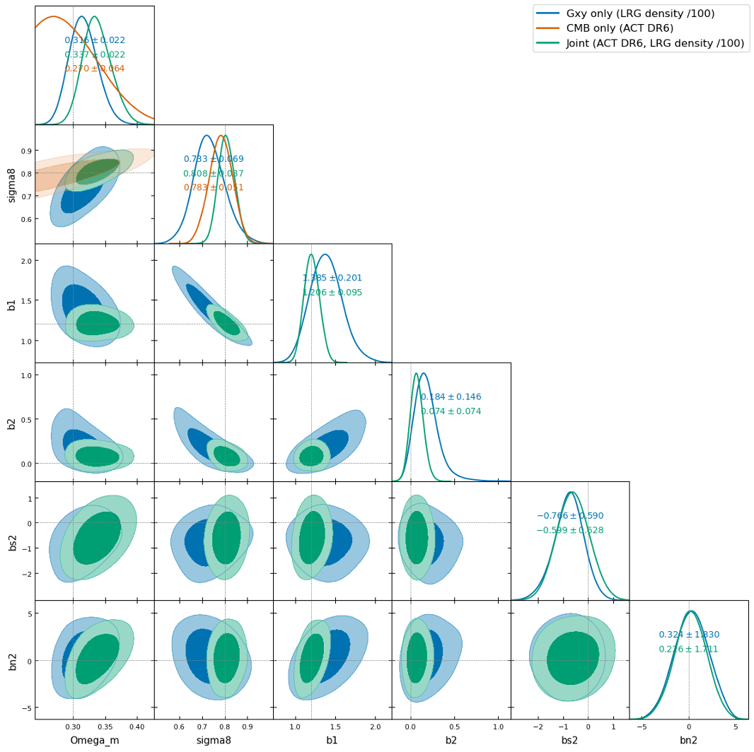
Validation on AbacusSummit ($\delta_L \mid \delta_g, \kappa$)
Implementation and inference of PNG ($f_\mathrm{NL}, \delta_L \mid \delta_g, \kappa$)

Breaking degeneracies

PRELIMINARY

(self-specified, ideal setting)

Ongoing:

Validation on AbacusSummit ($\delta_L \mid \delta_g, \kappa$)
Implementation and inference of PNG ($f_\mathrm{NL}, \delta_L \mid \delta_g, \kappa$)

Breaking degeneracies

PRELIMINARY

(self-specified, ideal setting)

Thank you!

hsimonfroy.github.io/hollved

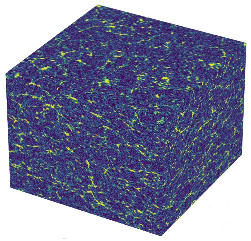
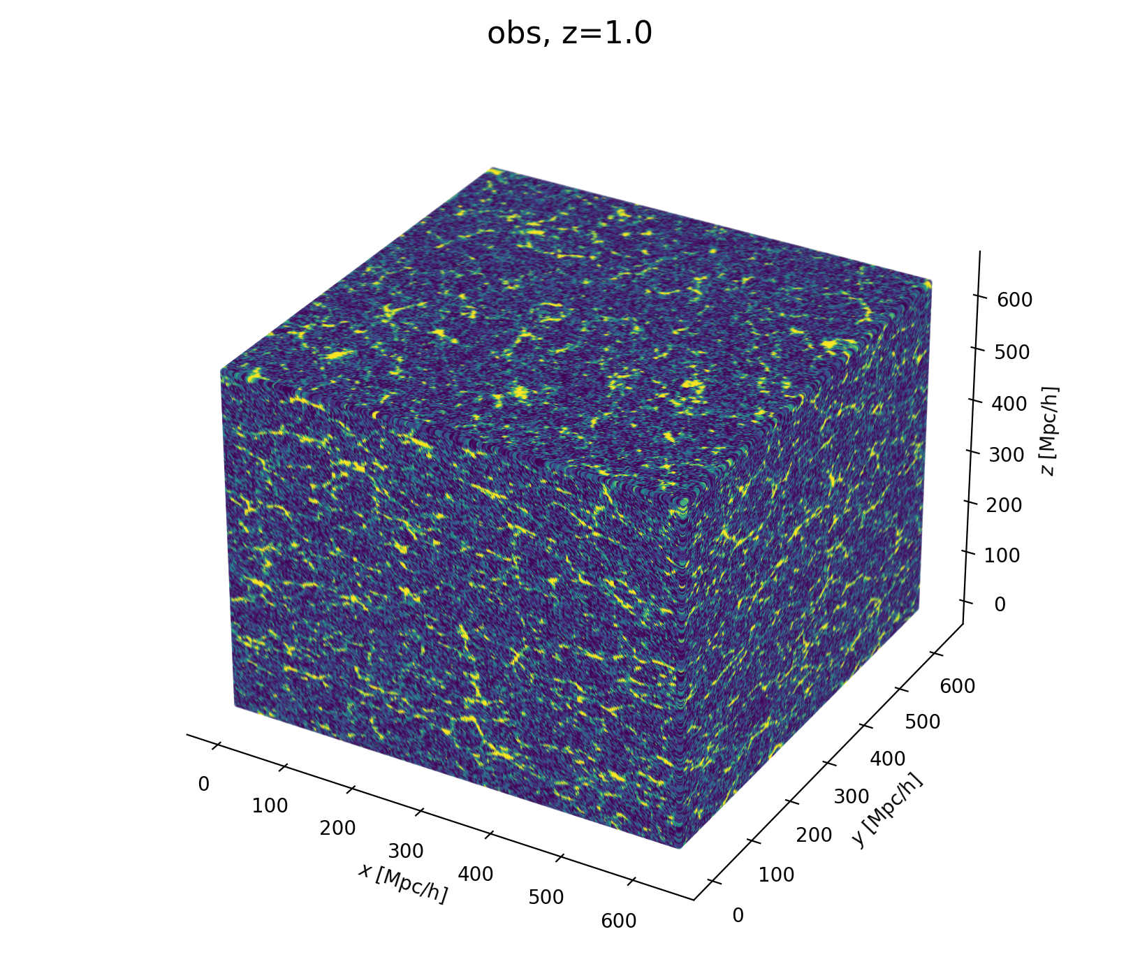
What it looks like

Inferring jointly cosmology, bias parameters, and initial matter field allows full universe history reconstruction

Simon+2025

million-dimensional inference:
4h on 1 GPU node vs. days/weeks for other codes

Different samplers and strategies used for field-level (e.g. Lavaux+2018, Bayer+2023). Additional comparisons required.
We provide a consistent benchmark for field-level from galaxy surveys. Build upon $\texttt{NumPyro}$ and $\texttt{BlackJAX}$.

Samplers comparison

= NUTS within Gibbs
= auto-tuned HMC

= adjusted MCHMC
= unadjusted Langevin MCHMC

10 times less evaluations required

Unadjusted microcanonical sampler outperforms any adjusted sampler

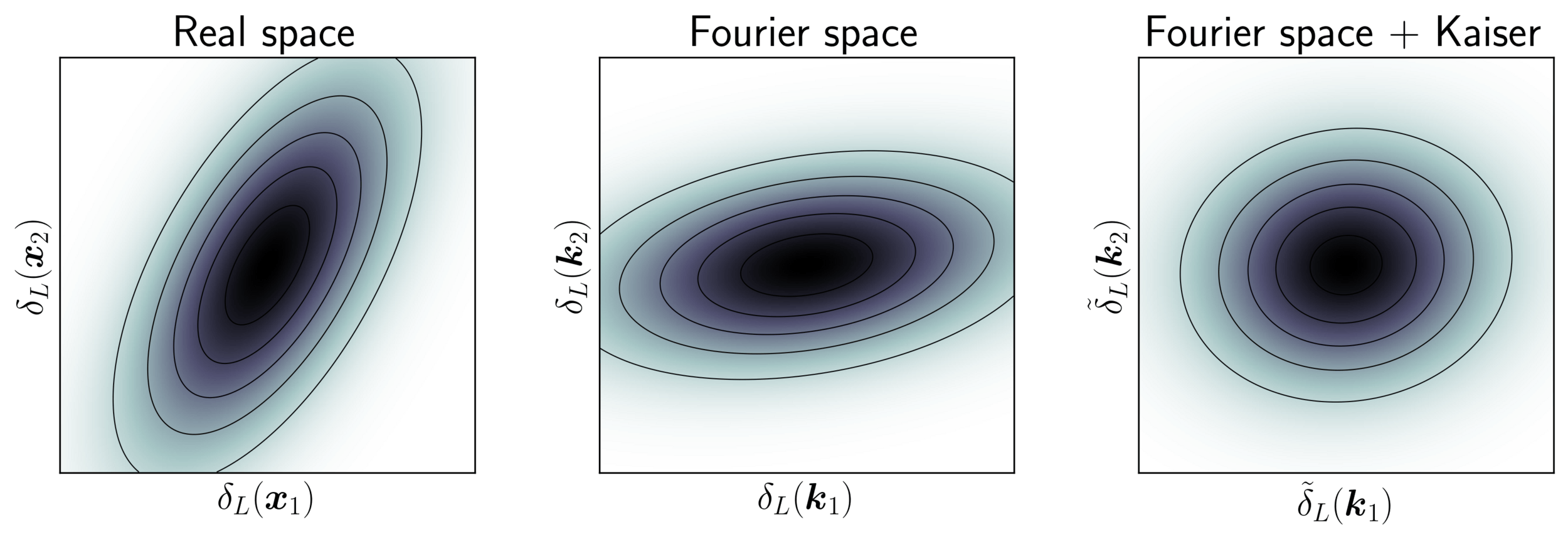
Model preconditioning

Sampling is easier when target density is isotropic Gaussian
The model is reparametrized assuming a tractable Kaiser model:
linear growth + linear Eulerian bias + flat sky RSD + Gaussian noise

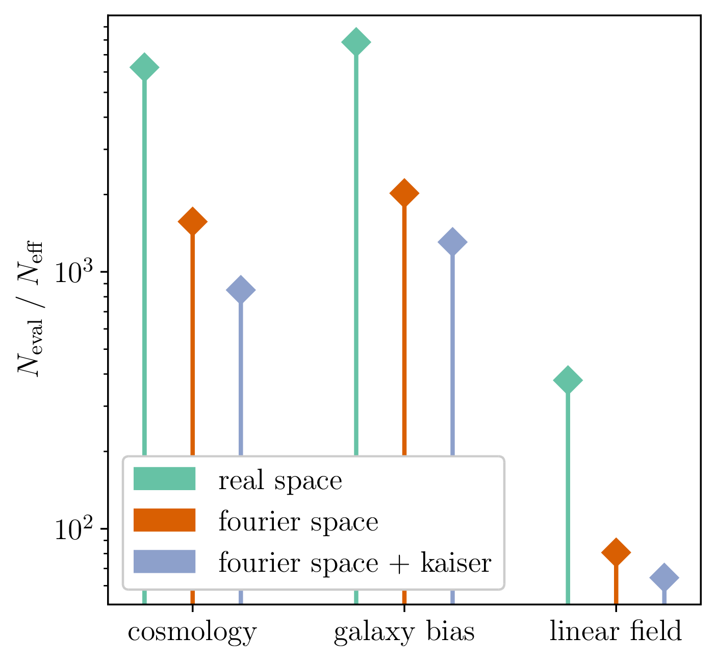
10 times less evaluations required

Benchmark results

Promising for future inferences, going multi-GPU using JaxDecomp
Code readily available at github.com/hsimonfroy/benchmark-field-level

Mildly dependent with respect to formation model and volume

Probing smaller scales could be harder

MCLMC sampler + field-level preconditioning assuming a linear Kaiser model:
4h on a 8GPU-node for $128^3$ PM inference

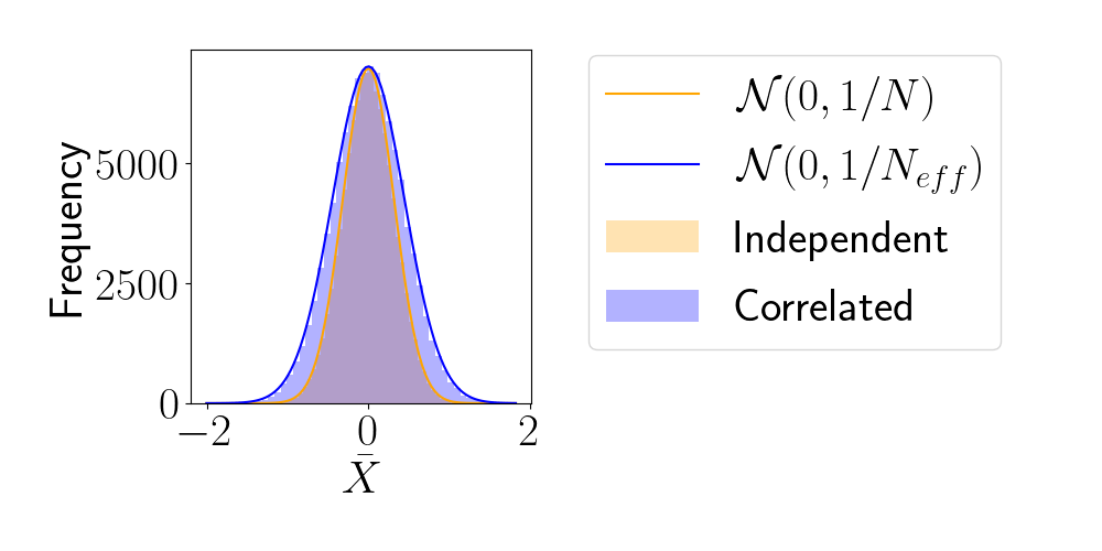
Effective Sample Size (ESS)
- number of i.i.d. samples that yield same statistical power.
- For sample sequence of size $N$ and autocorrelation $\rho$ $$N_\textrm{eff} = \frac{N}{1+2 \sum_{t=1}^{+\infty}\rho_t}$$so aim for as less correlated sample as possible.
Main limiting computational factor is model evaluation (e.g. N-body), so characterize MCMC efficiency by $N_\text{eval} / N_\text{eff}$

Andy Jones

How to compare samplers?

Tally

Currently visiting Montréal in Laurence Perreault-Levasseur team
Talks:
- Optimal cosmo information extraction at Sesto (for Euclid people)
- DESI meeting at Berkeley (for colab)
- CoBALt at Institut Pascal (for inflation theorists)
- Bayesian Deep Learning 3 at APC (for deep learners)
- ED Festival (for particle physicists)
- GDR Cophy 2h tutorial
Papers:
- stat paper at NeurIPS2024 (from master internship)
- Benchmarking Field-Level in review on JCAP
- PNG measurement at the field level in prep
Teaching: Bachelor 2 Biostats (20h) and Master 1 Maths (15) courses at UPsaclay
Formation:
- VSS, Science ethics, Sustainable dev. (Open Science left)
- Euclid summer school

Next steps

Scientific:
- Validation for PNG inference and application to DESI
- Alternative sampling method for field-level inference
- Going Multi-GPU
Manuscript:
- Detailed plan at the end of December, first chapter in January
Looking and applying for postdocs this Autumn,
hence the meetings and visits...

Hugo SIMON
PhD student supervised by
Arnaud DE MATTIA and François LANUSSE

Field-level Bayesian inference
High-dimensional sampling
Differentiable N-body simulations
Primordial non-Gaussianity from DESI

Hugo SIMON
PhD student supervised by
Arnaud DE MATTIA and François LANUSSE

Field-level Bayesian inference
High-dimensional sampling
Differentiable N-body simulations
Primordial non-Gaussianity from DESI

Hugo SIMON
PhD student at CEA Paris-Saclay, supervised by
Arnaud DE MATTIA and François LANUSSE

Field-level Bayesian inference
High-dimensional sampling
Differentiable N-body simulations
Primordial non-Gaussianity field-level inference from DESI

Field-Level Inference of Primordial Non-Gaussianity from DESI

The universe recipe (so far)

Cosmological inference

Cosmological inference

Two approaches to cosmological inference

Two approaches to cosmological inference

High-dimensional sampling is hard

Canonical/Microcanonical MCMC samplers

Samplers comparison

Benchmark results

At the end of the day

Field-Level modeling of PNG

Field-Level sampling

Field-Level Inference of PNG

Field-Level Inference of PNG

Toward more survey realism

Toward more survey realism on LRG SGC footprint

Field-Level Modeling

Field-Level Modeling and Inference

Field-Level Modeling and Inference

How to N-body-differentiate?

How to N-body-differentiate?

MCMC sampling

Canonical MCMC samplers

Microcanonical MCMC samplers

Afraid of unadjusted sampling?

Primordial Non-Gaussianity from galaxies

Probing inflation with galaxies

Field-Level modeling of PNG

Field-Level modeling of PNG

Field-Level modeling of PNG

Fitting AbacusSummit+HOD

Galaxy stochasticity

Preliminary FLI results on PNG

Preliminary FLI results on PNG

Probing inflation with FLI

Preliminary FLI results on PNG

Field-Level Multi-Probing

Think (of the CMB) outside the box

Breaking degeneracies

Breaking degeneracies

Thank you!

Thank you!

What it looks like

Samplers comparison

Model preconditioning

Benchmark results

How to compare samplers?

Tally

Next steps

Hugo SIMON PhD student supervised by Arnaud DE MATTIA and François LANUSSE

Hugo SIMON PhD student supervised by Arnaud DE MATTIA and François LANUSSE

Hugo SIMON PhD student at CEA Paris-Saclay, supervised by Arnaud DE MATTIA and François LANUSSE

Field-Level Inference of Primordial
Non-Gaussianity from DESI

Toward more survey realism
on LRG SGC footprint

Hugo SIMON
PhD student supervised by
Arnaud DE MATTIA and François LANUSSE

Hugo SIMON
PhD student supervised by
Arnaud DE MATTIA and François LANUSSE

Hugo SIMON
PhD student at CEA Paris-Saclay, supervised by
Arnaud DE MATTIA and François LANUSSE