Geometry, Algebra and Real World Robotics
Hugo Hadfield
2nd Dec 2024
Who am I?
- Robotics Research Software Engineer at NVIDIA SRL
- Automation/Robotics/Control/Estimation Engineer at Wayve
- PhD with Joan Lasenby on GA and robotics/computer vision/graphics
- Masters with Garth Wells in Monte Carlo scheduling with the Fenics Project
- Undergrad in Electrical/Information engineering at Cambridge University
- Cambridge Consultants electronics, microcontrollers, computer vision for medical devices




The Team

Trinity College
Cambridge University Signal Processing and Communications Laboratory

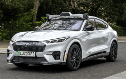
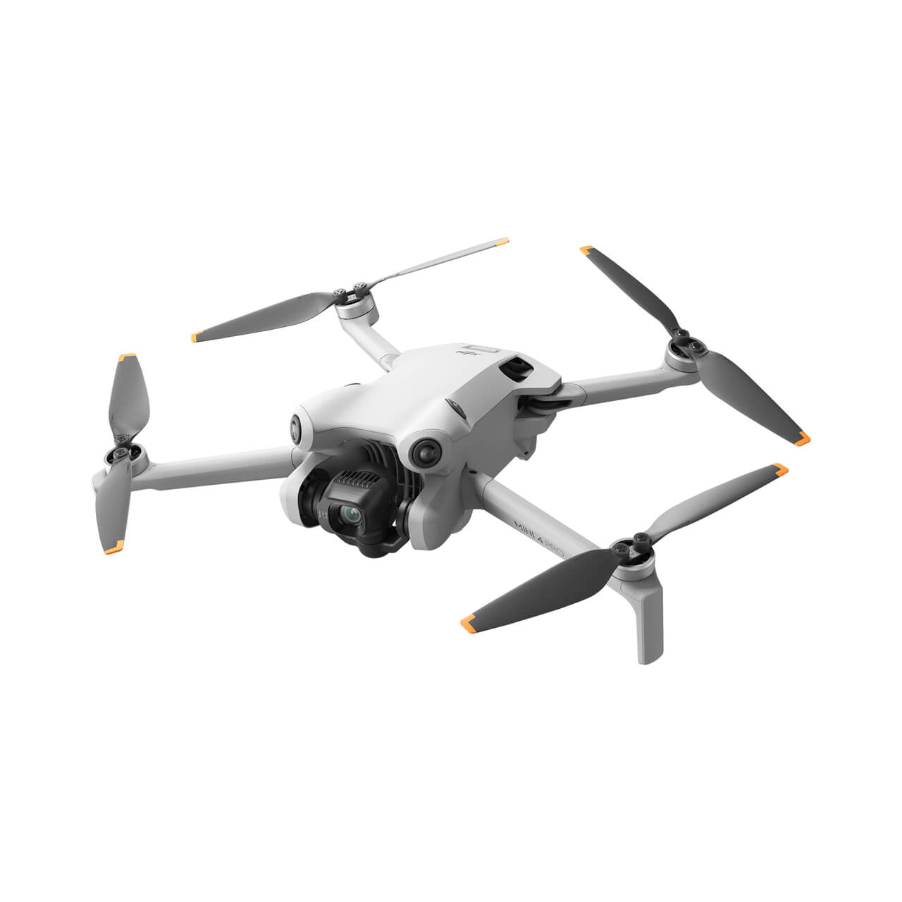
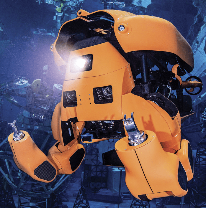
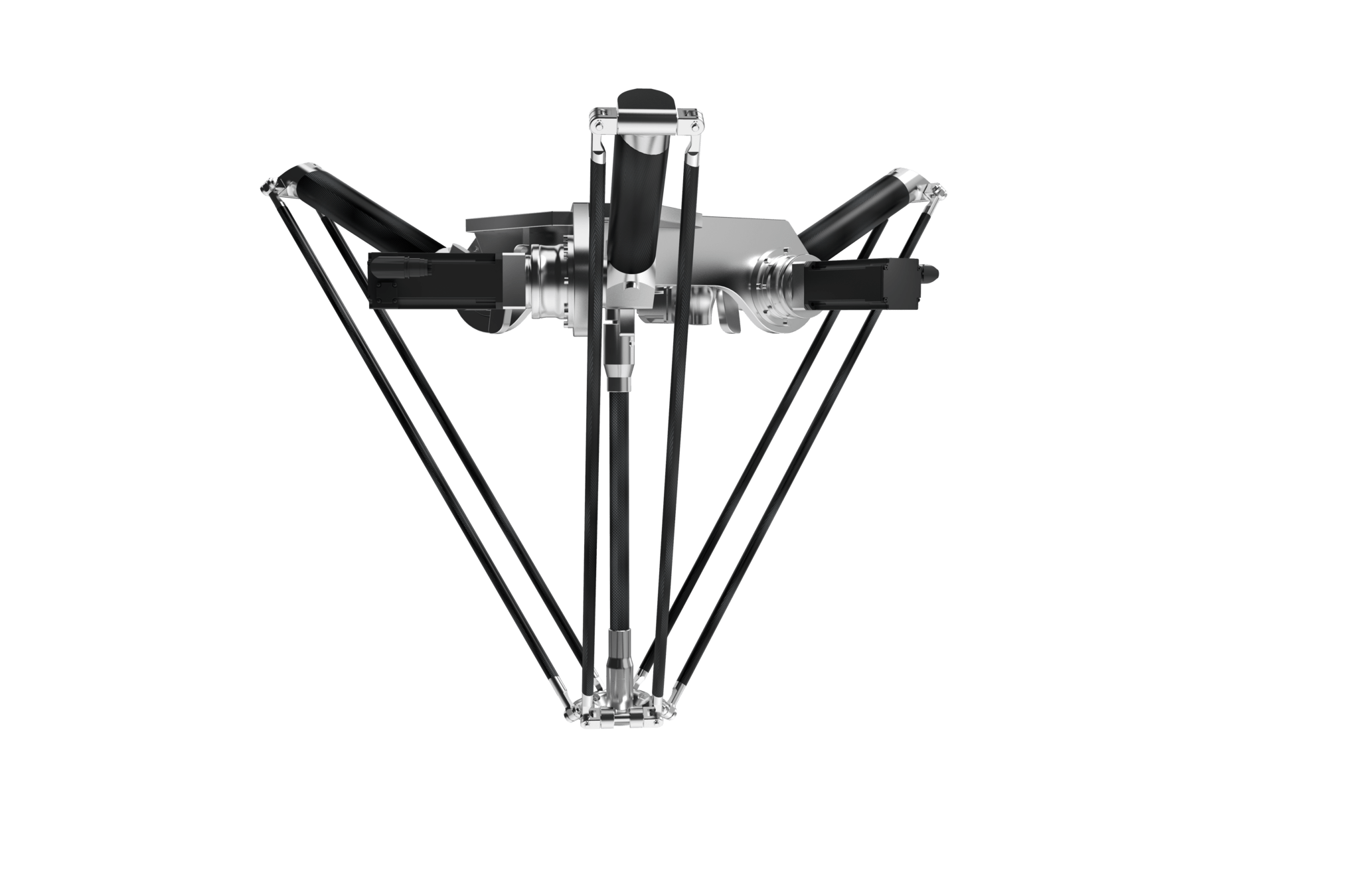
Robots out in the wild
- Articulated robotics
- Mobile robotics
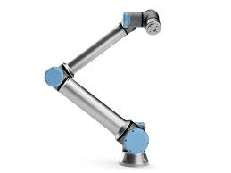

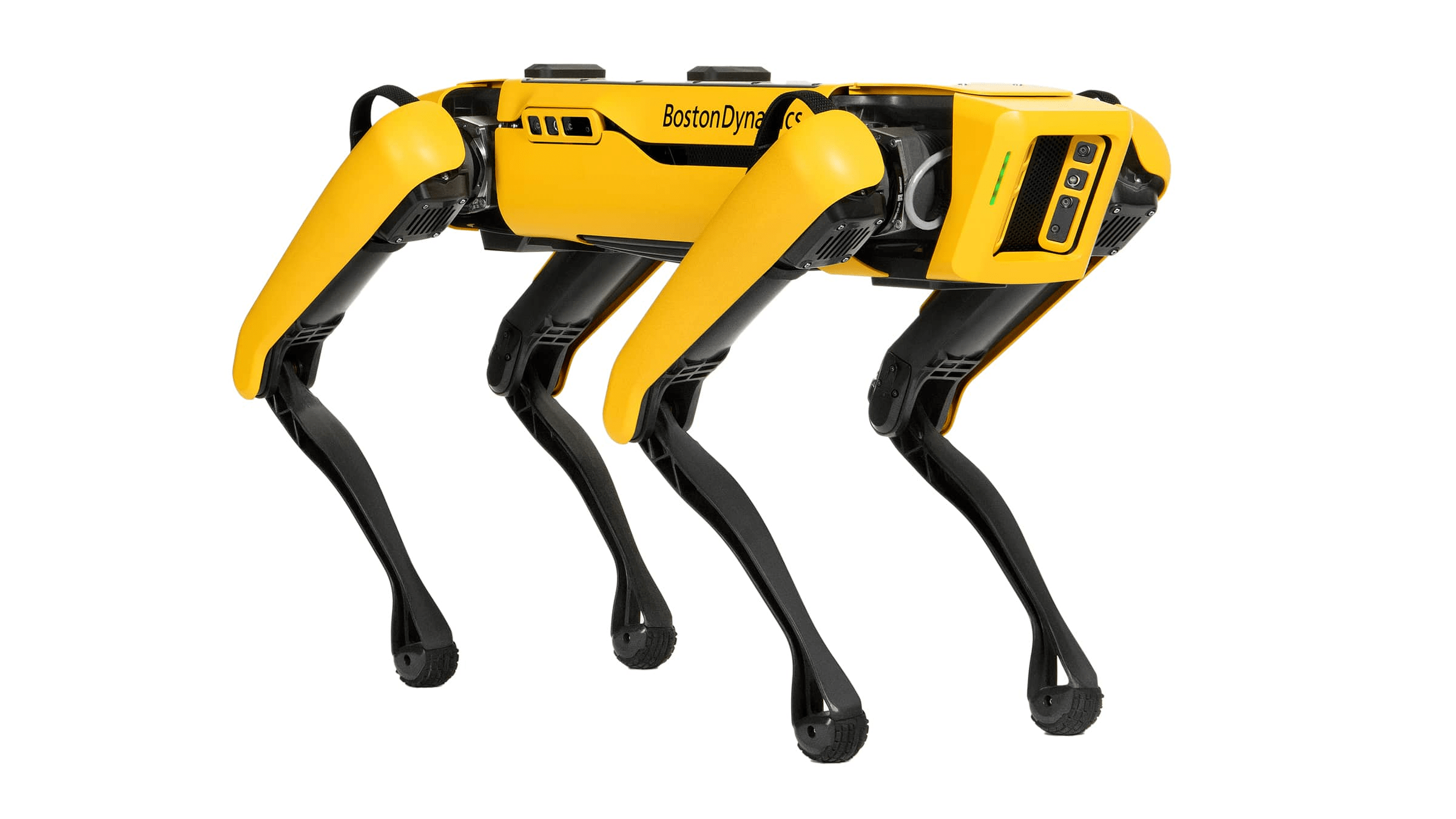
Articulated Robotics
- What do we do in our day-to-day:
- Transforming between 3D frames
- Manipulating transform objects
- Forward and inverse kinematics
- Motion planning
- Dynamics of articulated bodies
- Constrained motion
- Force, velocity and jerk calculations
- Locomotion simulations
Transforms and Frames
- Manipulation of Transforms and frames of reference is fundamental to robotics
- We need to be able to compose, decompose, optimise, differentiate these representations
-
- 3x3 matrices for rotation only
- 4x4 matrices for rotation and translation together
- quaternions for rotation only
- dual quaternions for rotation and translation together
- Cl(3) for rotation only
- Cl(3, 0, 1) for rotation + translation
- Cl(4, 1, 0) for rotation + translation + dilation
Algebras of Transforms
- What if we made algebras of transforms? Might make it easier to manipulate these objects etc.
- What would it take to make an algebra for rotation?
- What would it take to make an algebra for rotation and translation?
- What if we wanted to model space time transforms or other stuff?
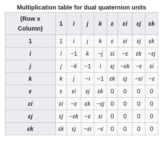
How are we actually going to deal with this in a computer?
- We need to store our transform objects somehow...
- What are our options?
- Store a list of the coefficients of each basis element and define some kind of operations between them
- Use some kind of matrix to represent each basis element and the coefficients. Use normal matrix operations
- This is effectively the fundamental split between many different libraries. Both of these approaches have pros and cons. The coefficient list approach is often minimal.
What does this have to do with GA?
- Different bits of Clifford subalgebras can be identified with the different elements of transformation groups.
- Clifford algebras already have products defined.
- Eg. 3D GA can do rotation:
- 1, e1^e2, e2^e3, e1^e3
- Eg. 3D P/CGA can do rotation and translation
- 1, e1^e2, e2^e3, e1^e3, e1^e_inf, e2^e_inf, e3^e_inf
- GA is useful here because not only does it have the transform elements in the algebra, but also the objects that you apply them to!
Serial Robot Forward Kinematics CGA
What if we want the full orientation of the endpoint?
Can we construct a rotor from origin to endpoint?
Construct the base rotors
Construct the first link's translation rotor
Construct the elbow and link 2 translation rotor
The combined rotor is the product of all of them
Just like chaining together 4x4 matrices
Time Derivatives
Consider a point transformed from the body frame to the world frame
Let's take some derivatives
Now we need to use the fact rotors are identity magnitude
The quantity
is often defined, this quantity is
always a bivector. This is the twist of the body.
These results are well known in Screw Theory
Constrained Dynamics of a Pendulum
P
Gravity
A simple rod pendulum is attached to a pivot point at one end. The pivot is at point P in the world frame.
In the body frame the point A is the attachment point. In the world frame this point is labelled P.
Forces as lines
Forces have a line of action, an orientation, and a magnitude
We can therefore naturally encode a force as an infinite line in CGA
force magnitude
force direction
3d point through which the line passes
Note we have used the dual construction of the line here, ie. F is a bivector
Wrenches: Forces and moments as screws
Both dual force lines and our bivector moments are screws, and specifically because they carry forces/moments they are known as wrenches (see [12])
If h is 0 then we have a force line
Iif m is 0 magnitude we have a pure moment
The general form of a screw is:
We can add and subtract screws at will and we will still stay on the screw manifold
Constraint via Virtual Power
Define an inertia tensor Q which transforms between body frame screw momentum and the body frame twist
The power done by a virtual wrench T acting against a body frame twist is given by this, where v is a scalar power:
In the case of a constraint, v must always be 0 as we do no work against it.
After doing an enormous amount of boring algebra we get this equation:
Pin Constraint
We now have an equation to solve for Wb:
We need to know what form T should take. For a pin constraint we can construct a virtual wrench that connects the centre of mass of the object C with the pivot point P.
Believe it or not, this is basically just Ax = b
Solving via Linear Algebra
Write the left hand side linear operator as M and the resulting multivector as N. Splitting W_b into S_b and F_b we get:
If we have a linear mapping of a multivector $M$ we can represent this mapping as a matrix of real coefficients \[c_{ij}$ acting on a vector of multivector coefficients for a given basis $X_i$ by the following construction:
And we can just solve this with whatever numerical linear algebra solver we like. As it is a point we will just pick a basis of any three perpendicular lines that go through the pivot point
Running the whole simulation
We can set up the whole simulation as follows:
And then we can plug it into whatever numerical ODE solver we like. For example, RK4.
Nothing fancy here, virtual power is a very old technique
We can also used Pinned Multivectors to do constraints
P
Gravity
Lots of algebra, easy to make mistakes in the setup of all of these constraint problems. I will send through a notebook with my implementation in case people are interested
Serial Robot Inverse Kinematics
(If \(P^2 < 0 \) then y is out of reach)
Construct a sphere at the base, \(n_0\)
Construct a sphere at the endpoint, y
Intersect the spheres to give a circle
Define a vertical plane through the endpoint and base
Intersect the circle and the plane to give a point pair
Choose one of the elbow position solutions
Model of a Delta Robot
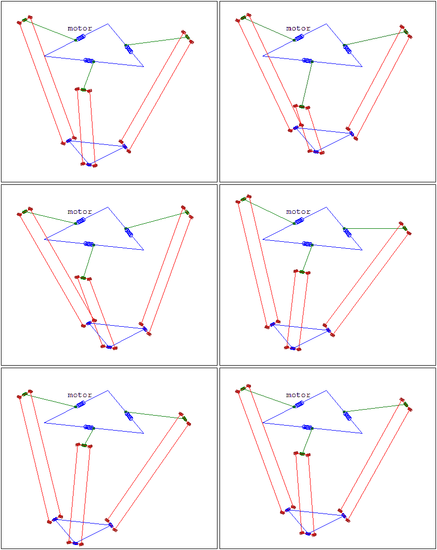
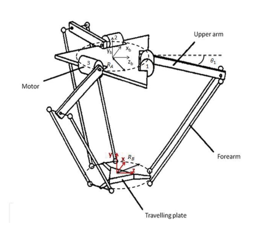
Forward Kinematics
Get the pseudo-elbow point \(A_i\)
Construct a sphere about the pseudo-elbow
The intersection of the three spheres (one from each limb) correspond to the two possible possitions of the centre of the end plate
Inverse Kinematics
If \(T_i^2 < 0\) then the target point is unreachable
Construct three possible elbow position circles
Construct three possible elbow position spheres
Intersect each sphere with its corresponding circle and select one possible intersection solution per limb
Finally get the motor angles
Articulated Robotics
- What do we do in our day-to-day:
- Transforming between 3D frames
- Manipulating transform objects
- Forward and inverse kinematics
- Motion planning
- Dynamics of articulated bodies
- Constrained motion
- Force, velocity and jerk calculations
- Locomotion simulations
Mobile Robotics
-
What do we do in our day-to-day:
- Transforming between 3D frames
- Manipulating transform objects
- Tracking objects on manifolds
- Optimisation on manifolds
- Modelling of cameras and sensors (triangulation etc.)
- Trilateration (GPS positioning algorithm)
Tracking Objects on Manifolds
R_t
An object moves along a path with a time varying rotor.
We wish to track its motion.
We observe frames along its length
Process Model
We can set up a state space model to track the object using a constant momentum process.
If you don't know the mass of the object just guess 1kg and spherical distribution of mass.
Observation Model
Never observe the rotation object directly, always observe its action on an object. Periodicity is annoying here.
Imagine the transform acts on a few test vectors, calculate where they would be. Compare that with the positions your measured transform would put them at. Do residuals in position space.
Optimisation on Manifolds
Imagine we have some cost function and we want to know where it is minimised but we want to optimise to find the rotor that works best.
Eg. Reprojection error in 3D SLAM
We can simply parameterise this in bivector space. Then solve by wrapping in scipy.optimize.minimize
Triangulation
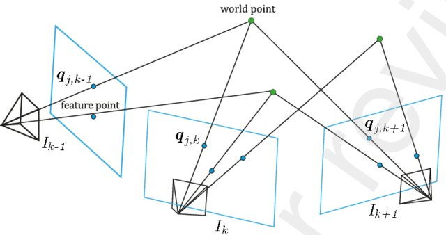
Trilateration
Mobile Robotics
-
What do we do in our day-to-day:
- Transforming between 3D frames
- Manipulating transform objects
- Tracking objects on manifolds
- Optimisation on manifolds
- Modelling of cameras and sensors (triangulation etc.)
- Trilateration (GPS positioning algorithm)
Why are you doing these problems in GA?
- No algorithm we have discussed today is new
- Once you are used to re-framing problems into the GA framework it becomes relatively fast and easy to learn new fields. Important for interdisciplinary areas like robotics.
- GA has not solved all my problems, but it has let me tackle significantly more than I could before.
Pros and Cons of GA in industry
- Pros:
- It is easy to glue together algorithms from many different fields
- If you know transform representations well you are instantly the go-to person for it in your company
- Its easy to see through the "fluff" of papers where they pretend to do fancy math just to write a paper
- Cons:
- People do not know about quaternions/dual quats let alone Cl(4,1,0) (and they shouldn't have to)
Pitfalls to be aware of
- Do not trust your derivations without numerical proof (not (just) mathematical proof, show me software tests)
- Do not try to force everyone you work with to use a niche mathematical representation directly (if people do not understand the code, the team will be inefficient)
- Do not believe people who tell you they have invented something new and it is revolutionary (these fields are very old, there is lots of material in the screw theory literature, go read it)
- Making something work robustly is more important (and harder) than phrasing it neatly in a nice framework

