2024年5月17日, 17:05-17:20
2024 年重庆引力与天体物理学术研讨会 · 重庆邮电大学
Exploring the Frontiers of Parameter Estimation with AI in Gravitational Wave Research
王赫 (He Wang)
hewang@ucas.ac.cn
中国科学院大学 · 国际理论物理中心(亚太地区)
中国科学院大学 · 引力波宇宙太极实验室(北京/杭州)



In cooperation with
Z.Cao, Z.Ren, M.Du, B.Liang, P.Xu, Z.Luo, Y.Wu, et al.
- non-GW
- NeuTra-lizing Bad Geometry in Hamiltonian Monte Carlo Using Neural Transport (1903.03704 )
- Accelerated Bayesian inference using deep learning (https://doi.org/10.1093/mnras/staa1469)
- Nested Sampling Methods (2101.09675)
- pocoMC: A Python package for accelerated Bayesian inference in astronomy and cosmology (2207.05660)
- Parallelized Acquisition for Active Learning using Monte Carlo Sampling (2305.19267)
- NAUTILUS: boosting Bayesian importance nested sampling with deep learning (2306.16923)
- Improving Gradient-guided Nested Sampling for Posterior Inference (2312.03911)
- floZ: Evidence estimation from posterior samples with normalizing flows (2404.12294)
- Deep Learning and genetic algorithms for cosmological Bayesian inference speed-up (2405.03293)
- GW
- Nested Sampling with Normalising Flows for Gravitational-Wave Inference (2102.11056)
- Bilby-MCMC: an MCMC sampler for gravitational-wave (2106.08730)
- Nested sampling for physical scientists (2205.15570)
- Fast gravitational wave parameter estimation without compromises (2302.05333)
- Importance nested sampling with normalising flows (2302.08526)
- Neural density estimation for Galactic Binaries in LISA data analysis (2402.13701)
- Robust parameter estimation within minutes on gravitational wave signals from binary neutron star inspirals (2404.11397)
10+5 = 15min
space-based (2)
what is flow and flow-based (4)
how flow can be used in MCMC.
mini Global-fit + flow
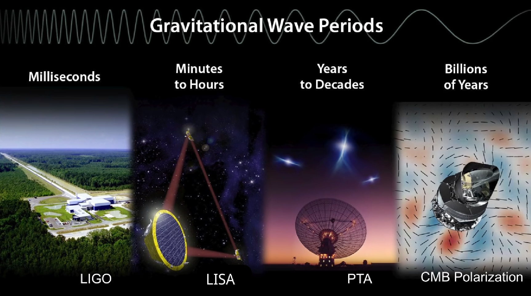
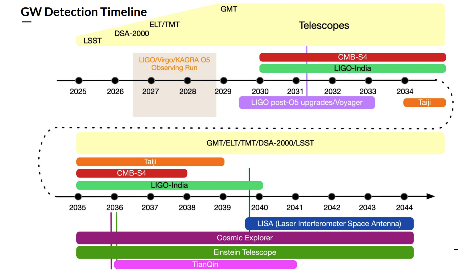
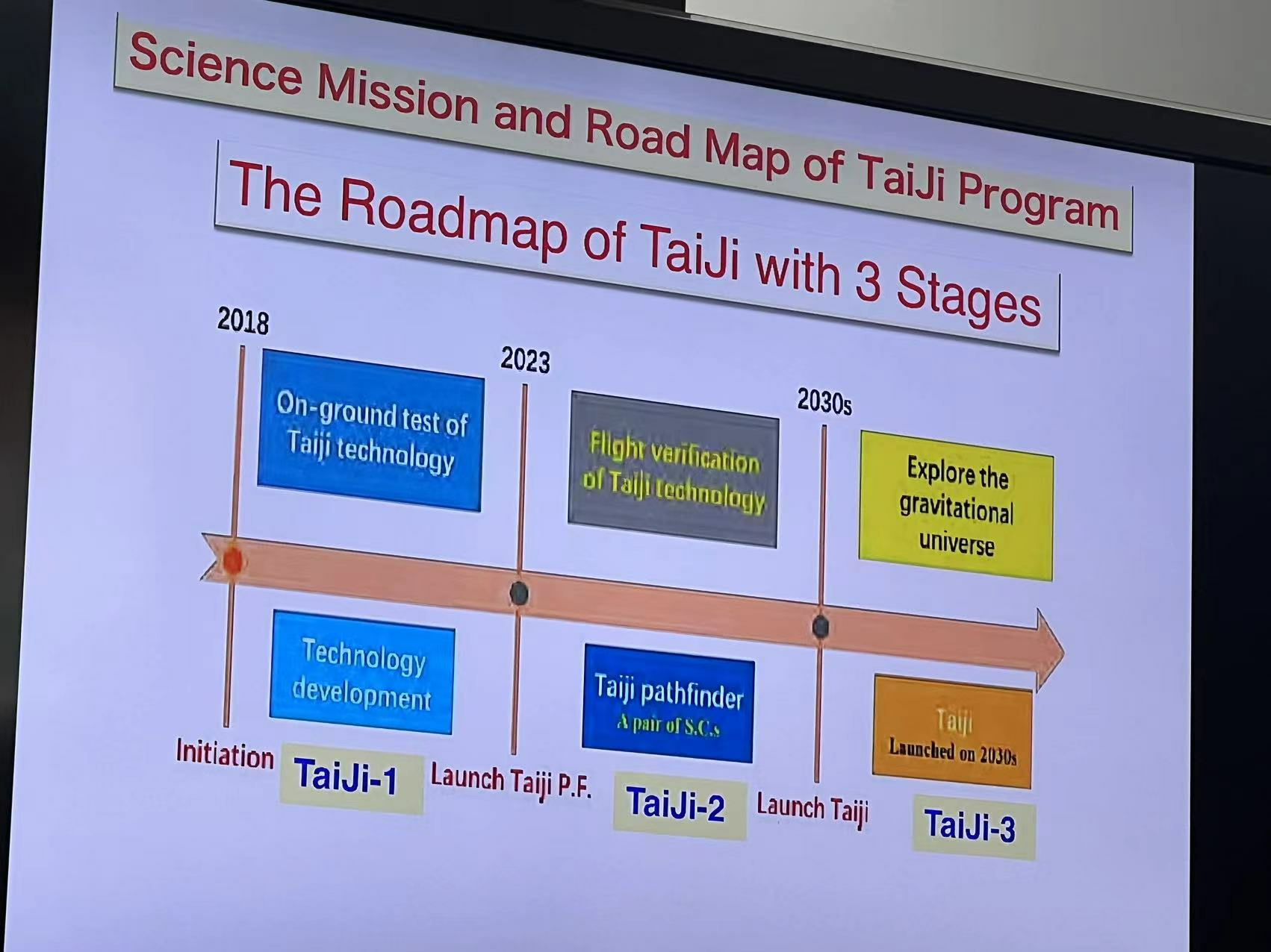
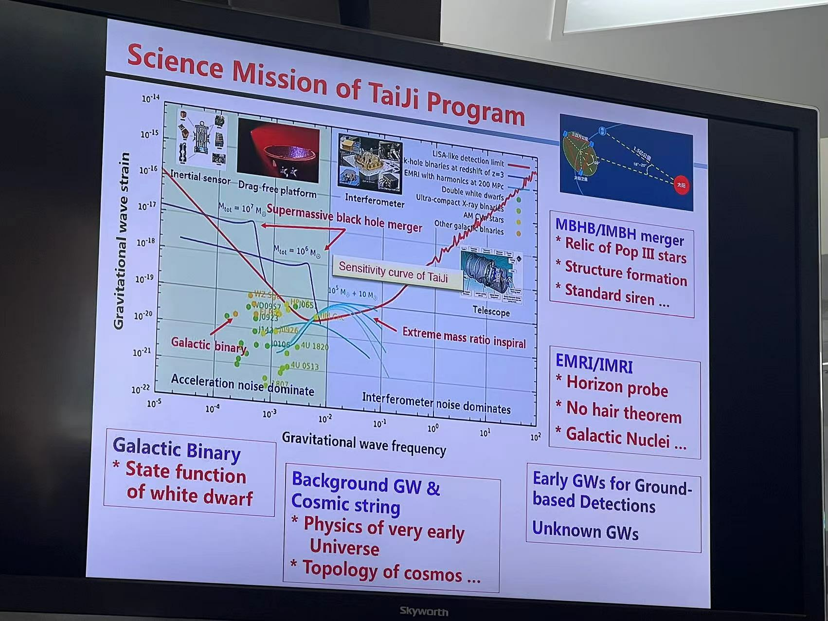
Taiji
Tianqin
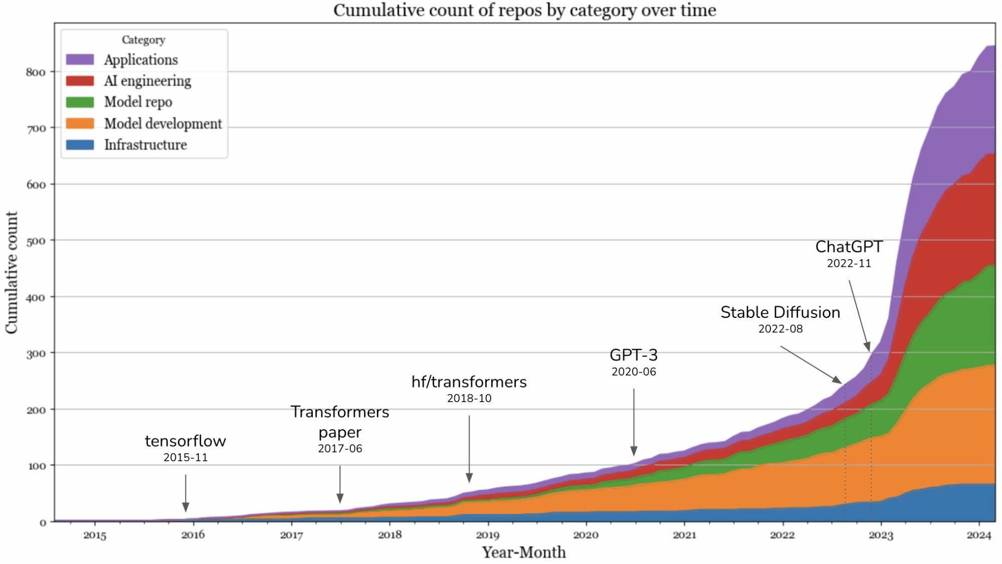
https://twitter.com/chipro/status/1768388213008445837?s=46&t=JmDXWgIucgr_FlsBFTvuRQ
DINGO+SEOBNRv4EHM找了3个ebbh
Evidence for eccentricity in the population of binary black holes observed by LIGO-Virgo-KAGRA
https://dcc.ligo.org/LIGO-G2400750
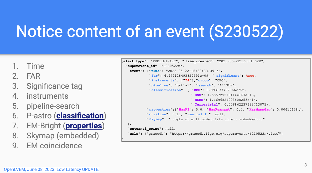
BEFORE
AFTER
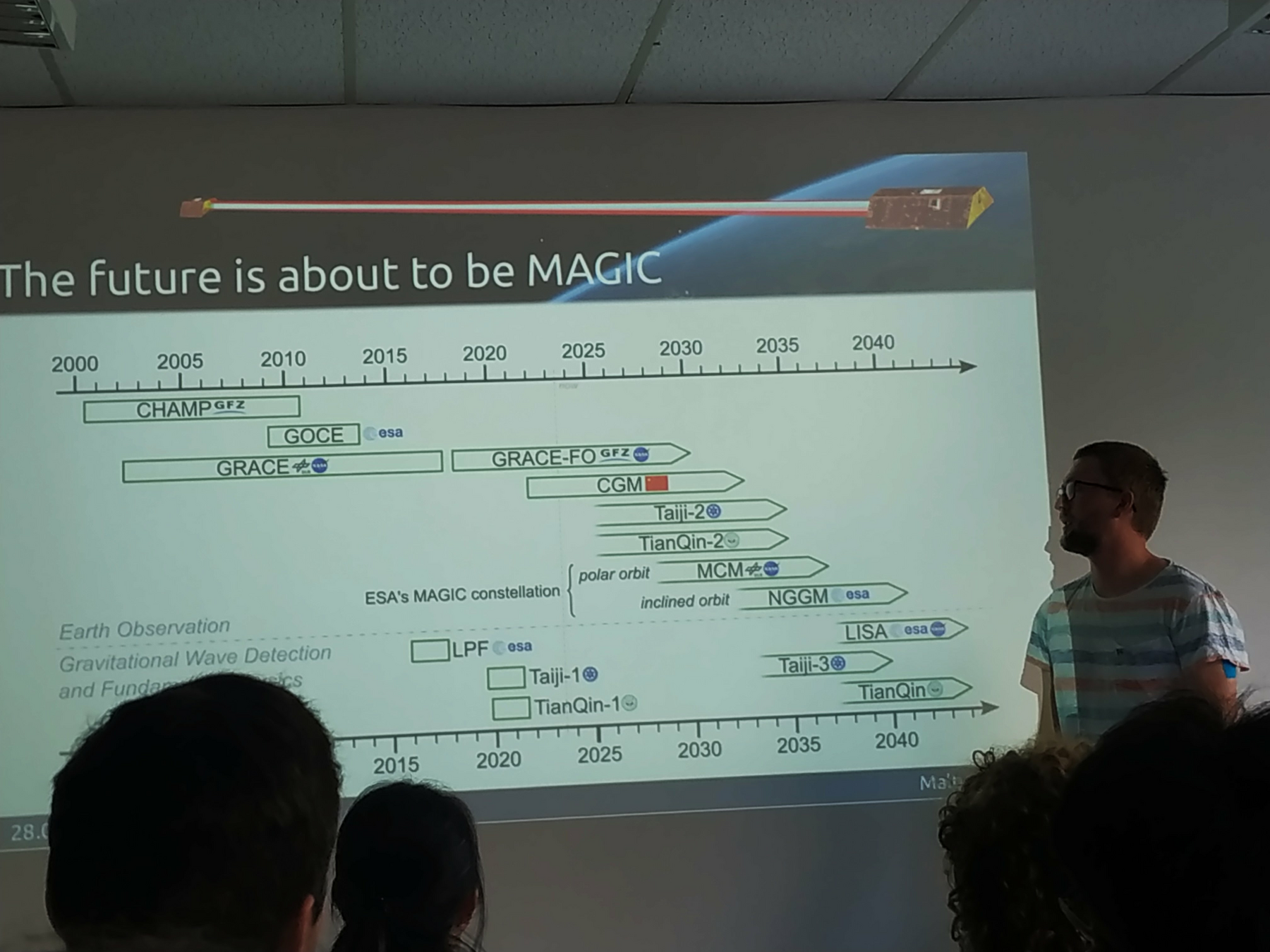
LIGO-G2300554

-
In 1916, A. Einstein proposed the GR and predicted the existence of GW.
-
Gravitational waves (GW) are a strong field effect in the GR.
-
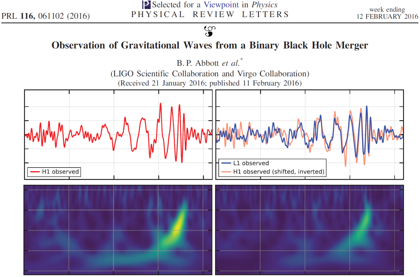
2015: the first experimental detection of GW from the merger of two black holes was achieved.
-
2017: the first multi-messenger detection of a BNS signal was achieved, marking the beginning of multi-messenger astronomy.
-
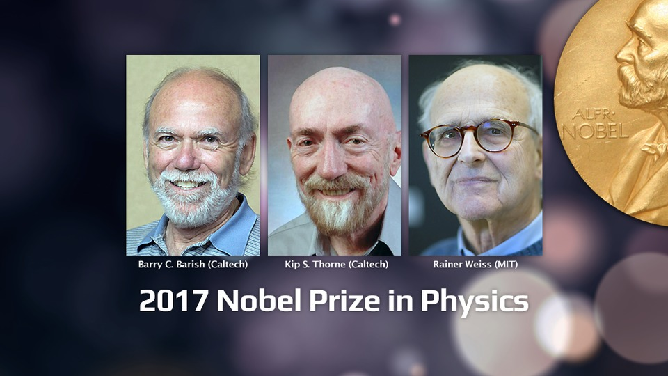
2017: the Nobel Prize in Physics was awarded for the detection of GW.
-
As of now: more than 90 gravitational wave events have been discovered.
-
O4, which began on May 24th 2023, is currently in progress.
-
Gravitational Wave Astronomy
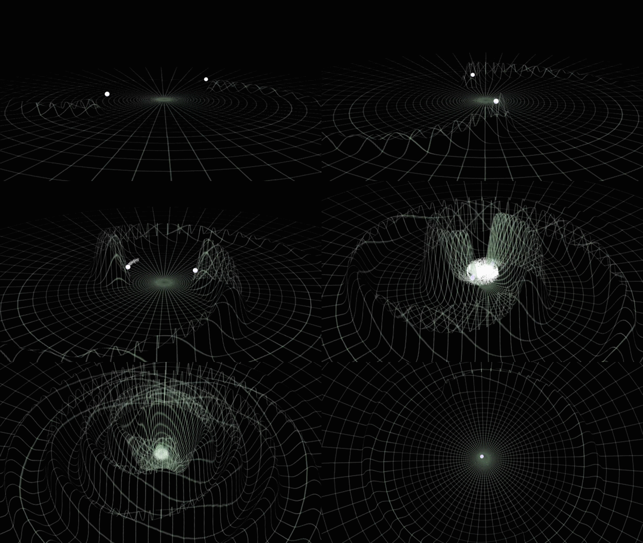

Gravitational waves generated by binary black holes system
GW detector

Gravitational Wave Astronomy
-
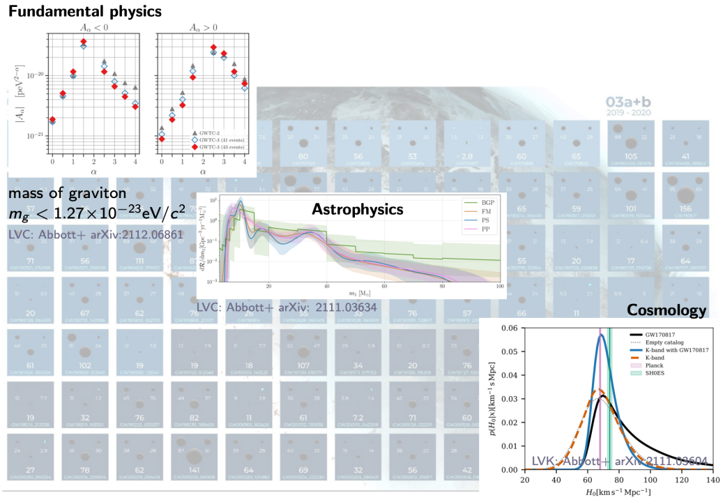
Fundamental Physics
- Existence of gravitational waves
- To put constraints on the properties of gravitons
-
Astrophysics
- Refine our understanding of stellar evolution
- and the behavior of matter under extreme conditions.
-
Cosmology
- The measurement of the Hubble constant
- Dark energy
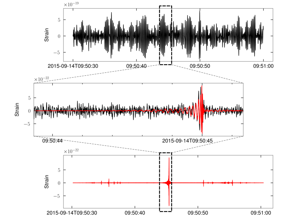
The first GW event of GW150914
Parameter estimation · Scientific discovery

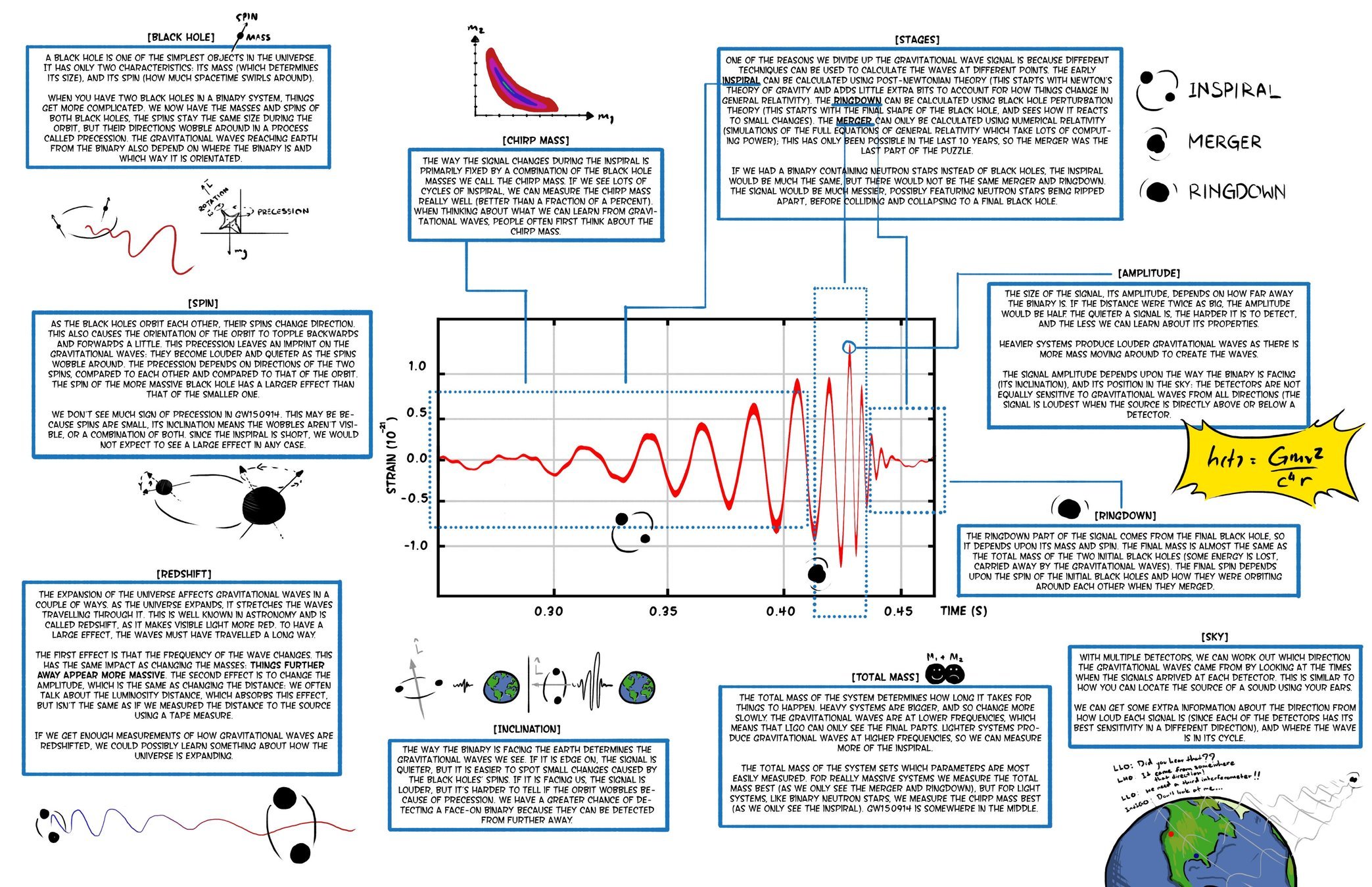
Credit: LIGO Magazine.
-
Traditional parameter estimation (PE) techniques rely on Bayesian analysis methods (posteriors + evidence)
- Computing the full 15-dimensional posterior distribution estimate is very time-consuming:
- Calculating likelihood function
- Template generation time-consuming
- Machine learning algorithms are expected to speed up!
Challenges of Parameter Estimation for GW


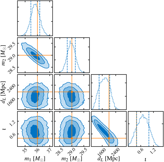
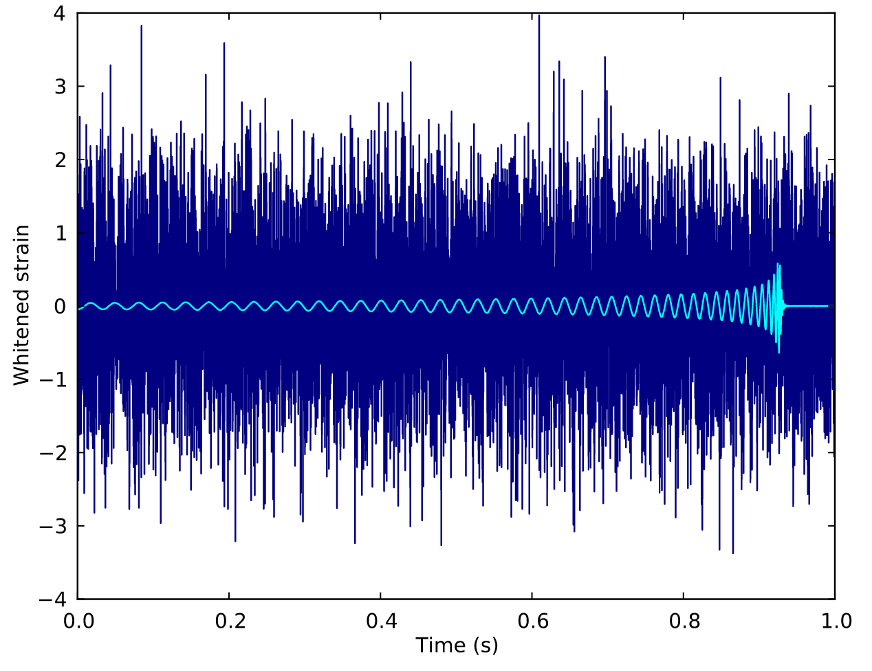
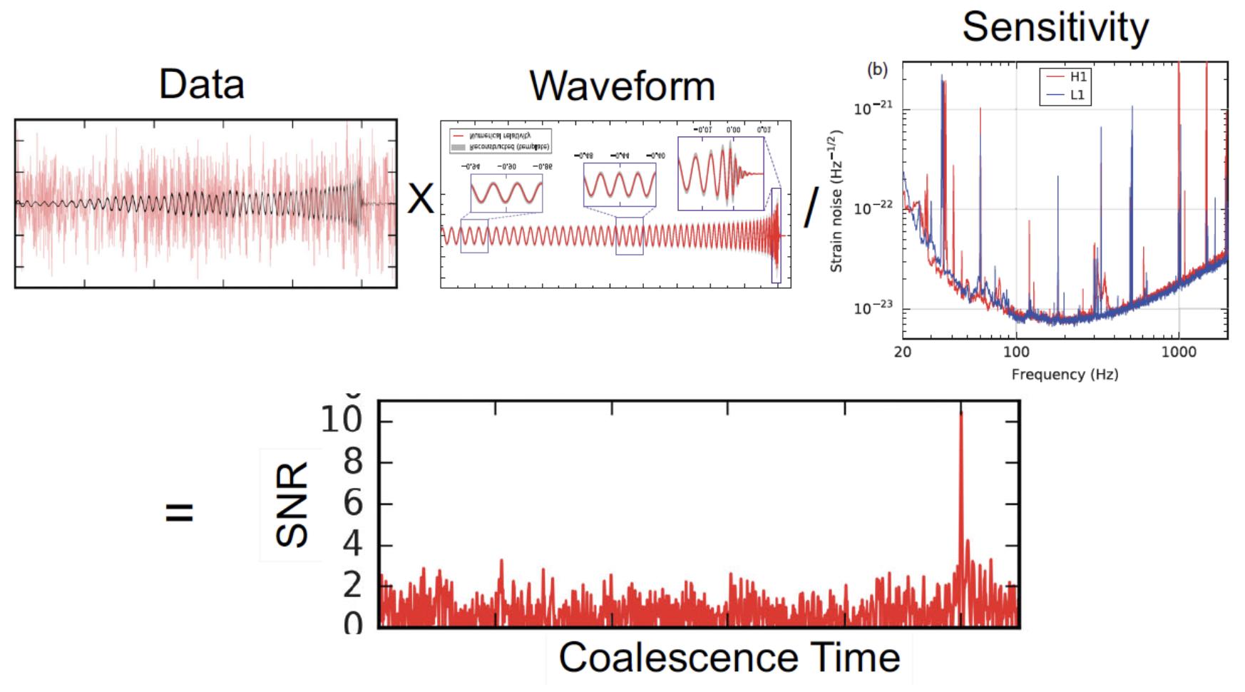
Bayesian statistics

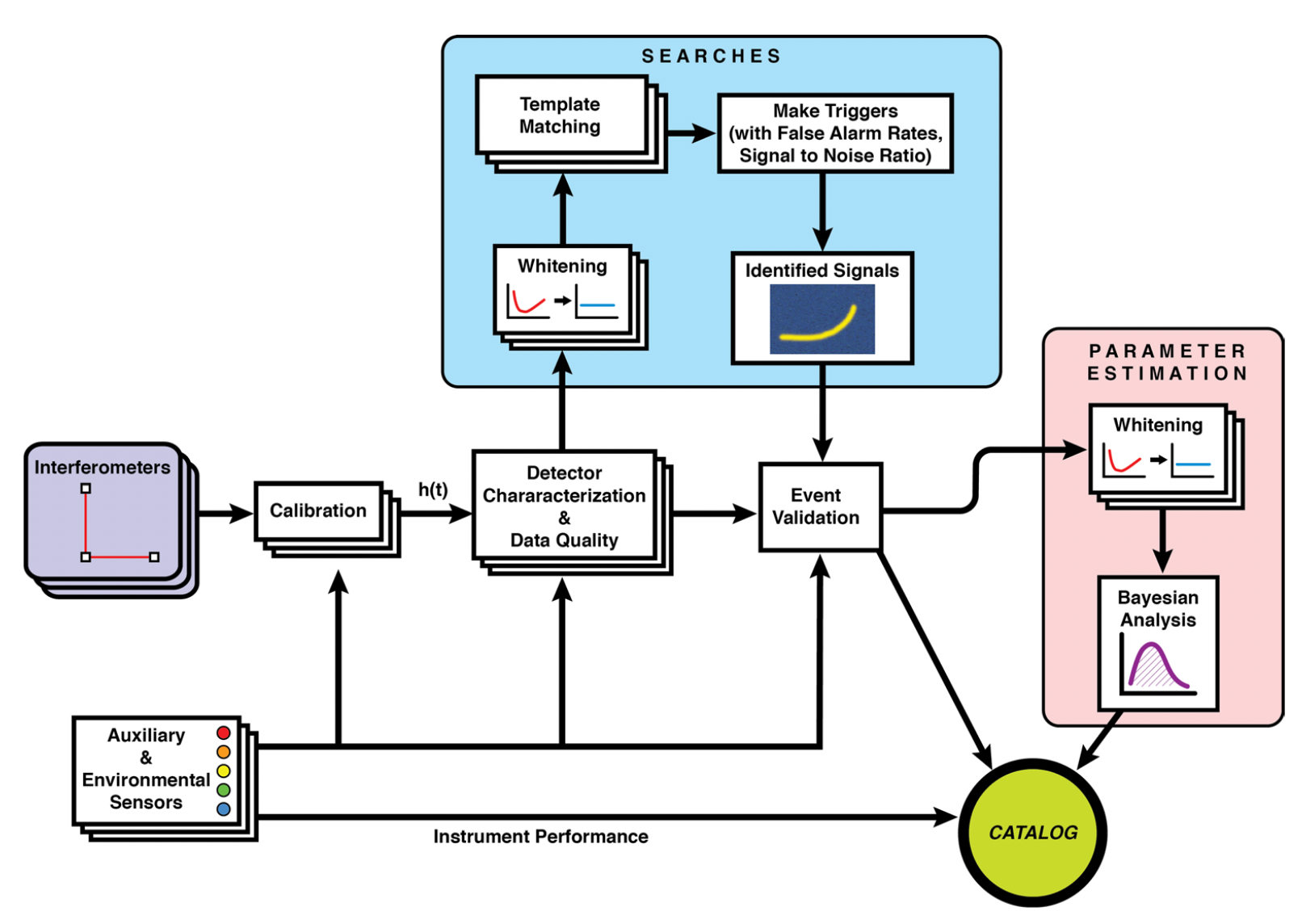
Data quality improvement
Credit: Marco Cavaglià
LIGO-Virgo data processing
GW searches
Astrophsical interpretation of GW sources
AI for Gravitational Wave: Parameter Estimation
- A complete 15-dimensional posterior probability distribution, taking about 1 s (<< \(10^4\) s).
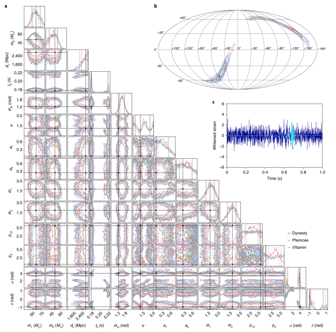
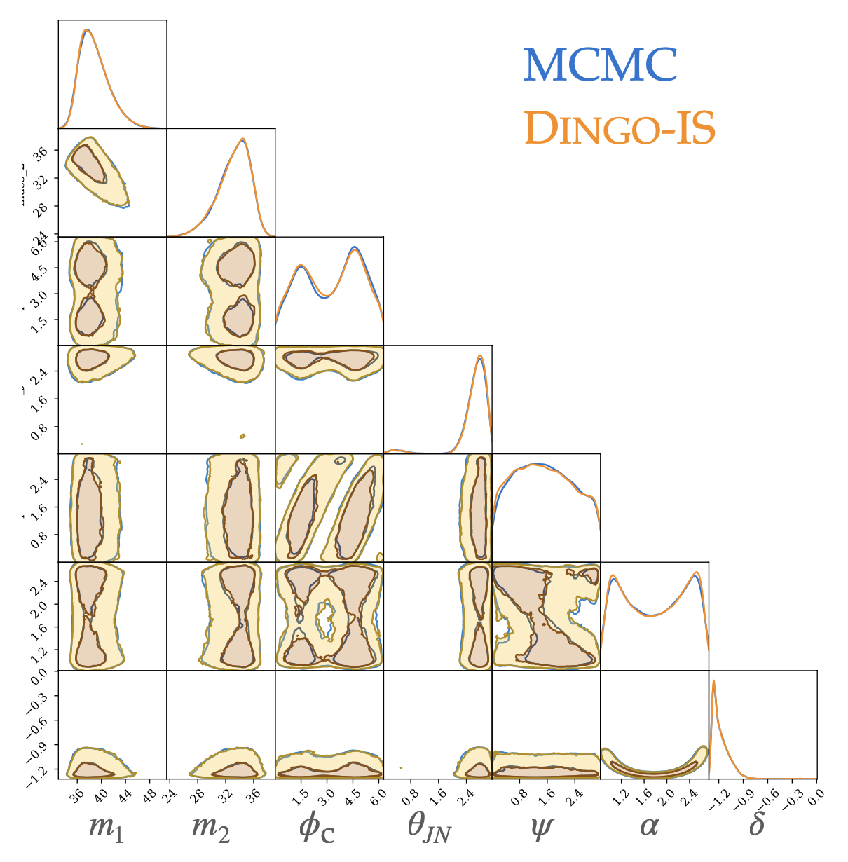
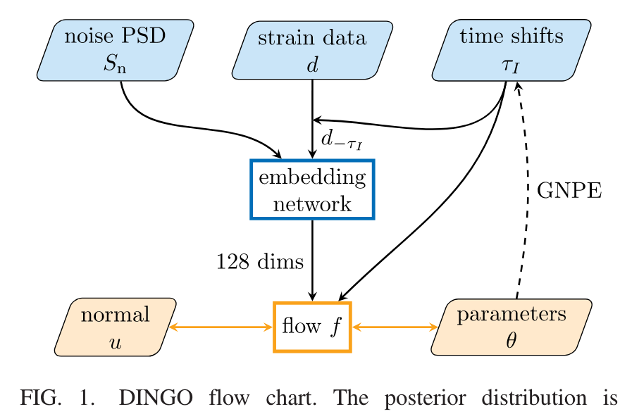
- Prior Sampling: 50,000 Posterior samples in approximately 8 Seconds.
- Capable of calculating evidence
- Processing time: (using 64 CPU cores)
- less than 1 hour with IMRPhenomXPHM,
- approximately 10 hours with SEOBNRv4PHM
PRL 127, 24 (2021) 241103.
PRL 130, 17 (2023) 171403.
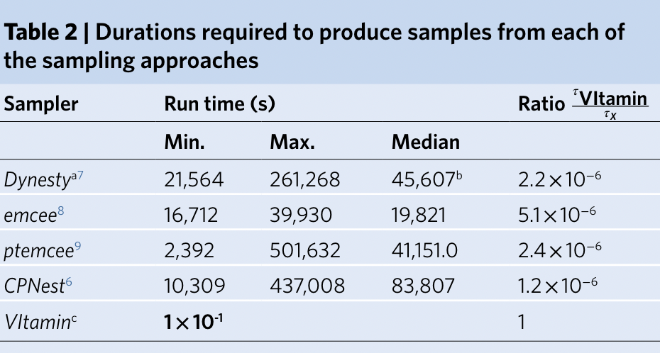
Nature Physics 18, 1 (2022) 112–17
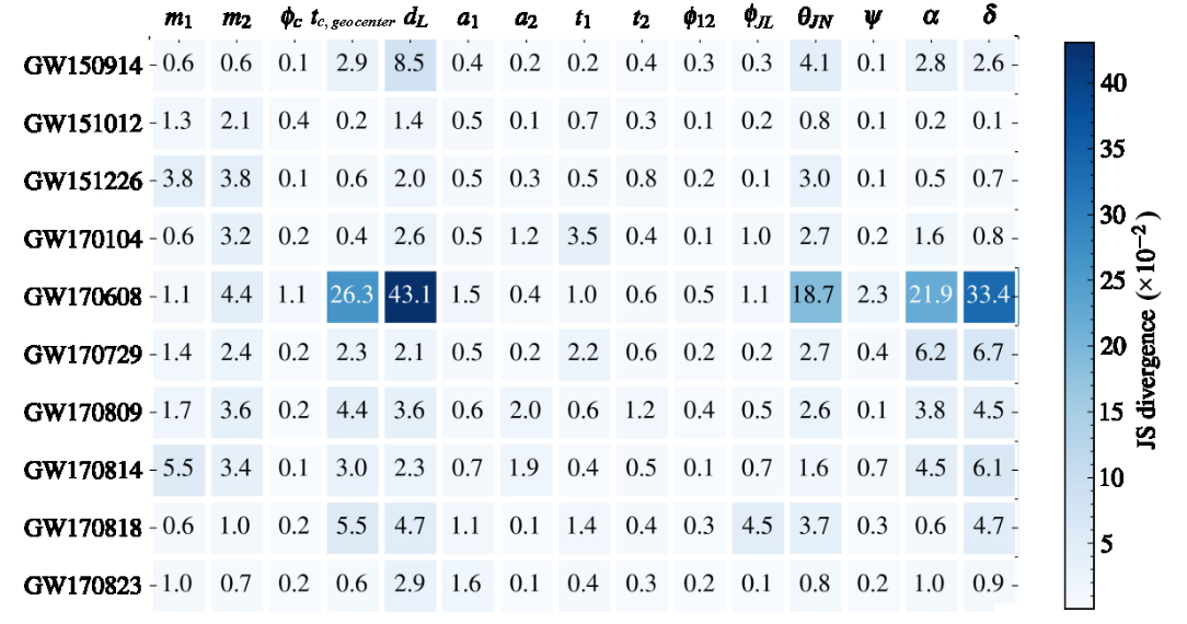
HW, et al. Big Data Mining and Analytics 5, 1 (2021) 53–63.
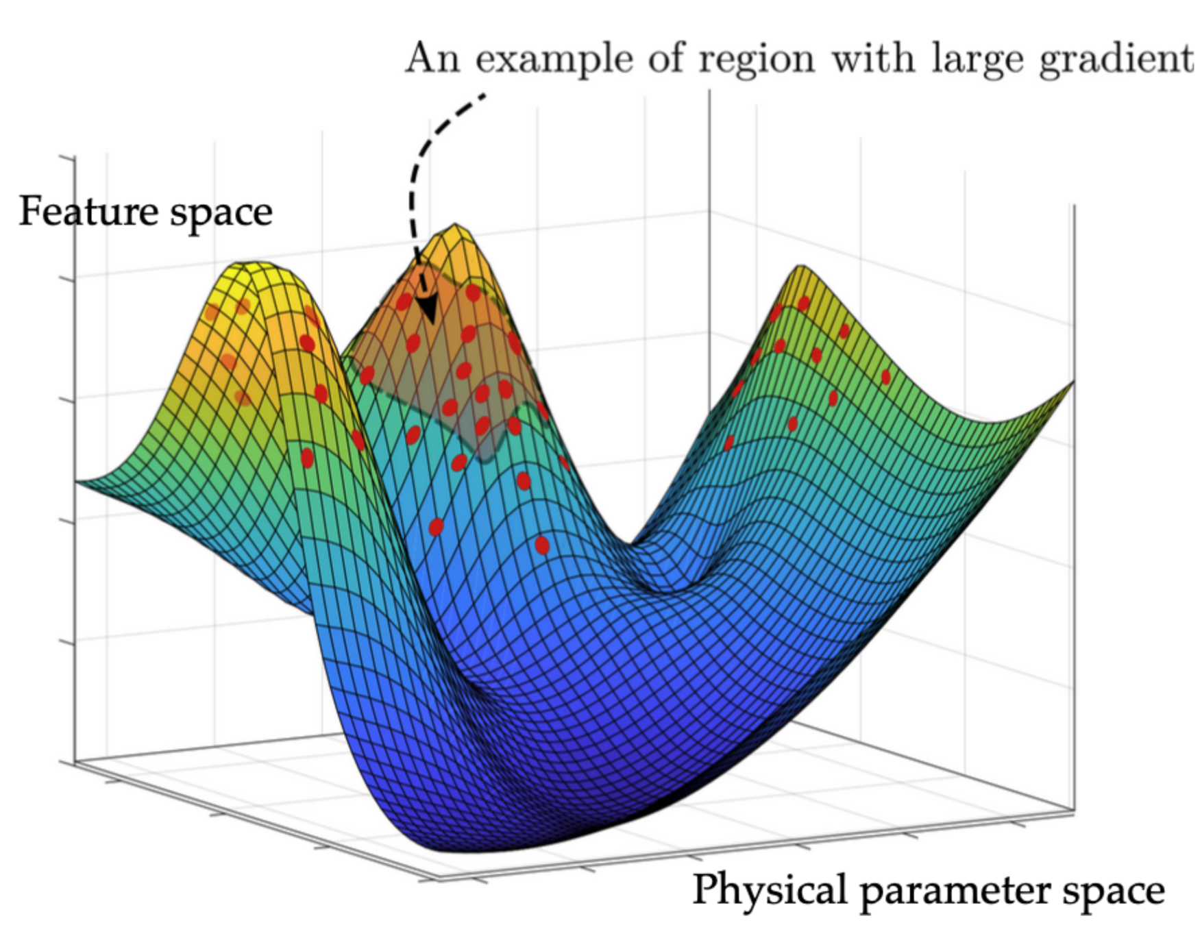
A diagram of prior sampling between feature space and physical parameter space

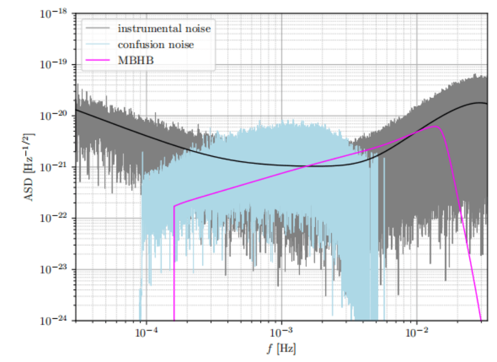
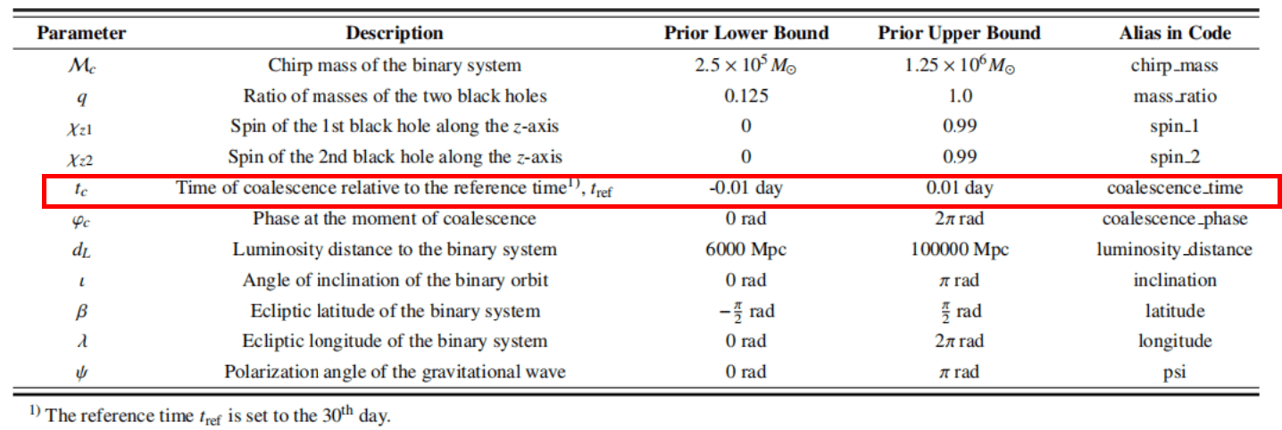
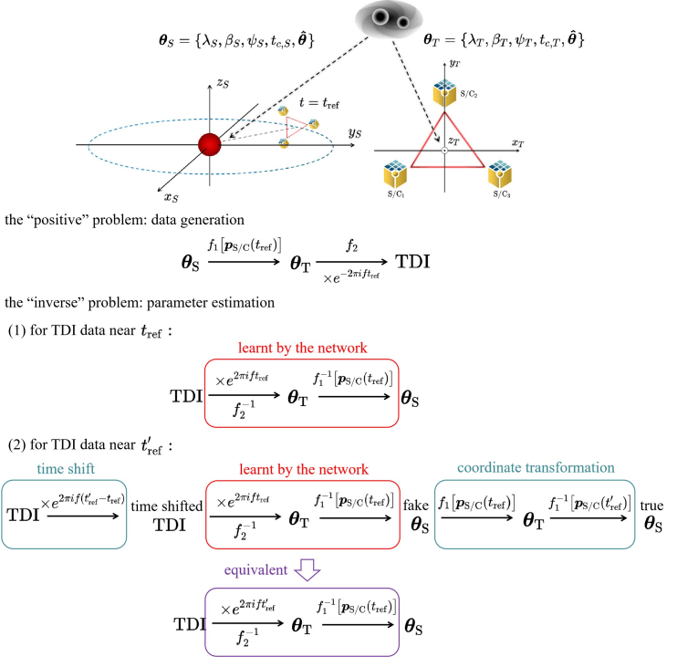
Rapid PE for Space-borne GW Detection

-
Data curation
-
Model: frequency domain, PhenomD, TDI-A,E response
-
Data:1 day, 15s per sample, shape=(2, 3, 2877)
-
Noise: Gaussian stationary from PSD + GB confusion noise
-
Project: Taiji program
-
M. Du, B. Liang, HW, P. Xu, Z. Luo, Y. Wu. SCPMA 67, 230412 (2024).
-
Motivation: To preprocess Global Fit data for early detection of merged electromagnetic observations for MBHBs.

(Based on 1912.02762)
The ABC of Normalizing Flow
The main idea of flow-based modeling is to express \(\mathbf{y}\in\mathbb{R}^D\) as a transformation \(T\) of a real vector \(\mathbf{z}\in\mathbb{R}^D\) sampled from \(p_{\mathrm{z}}(\mathbf{z})\):
Note: The invertible and differentiable transformation \(T\) and the base distribution \(p_{\mathrm{z}}(\mathbf{z})\) can have parameters \(\{\boldsymbol{\phi}, \boldsymbol{\psi}\}\) of their own, i.e. \( T_{\phi} \) and \(p_{\mathrm{z},\boldsymbol{\psi}}(\mathbf{z})\).
Change of Variables:
Equivalently,
The Jacobia \(J_{T}(\mathbf{u})\) is the \(D \times D\) matrix of all partial derivatives of \(T\) given by:
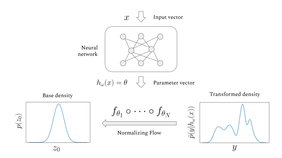

base density
target density

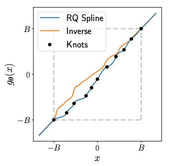
Rational Quadratic Neural Spline Flows (RQ-NSF)
(Based on 1912.02762)
- Data: target data \(\mathbf{y}\in\mathbb{R}^{11}\) (with condition data \(\mathbf{x}\)).
- Task:
- Fitting a flow-based model \(p_{\mathrm{y}}(\mathbf{y} ; \boldsymbol{\theta})\) to a target distribution \(p_{\mathrm{y}}^{*}(\mathbf{y})\)
- by minimizing KL divergence with respect to the model’s parameters \(\boldsymbol{\theta}=\{\boldsymbol{\phi}, \boldsymbol{\psi}\}\),
- where \(\boldsymbol{\phi}\) are the parameters of \(T\) and \(\boldsymbol{\psi}\) are the parameters of \(p_{\mathrm{z}}(\mathbf{z})=\mathcal{N}(0,\mathbb{I})\).
- Loss function:
- Assuming we have a set of samples \(\left\{\mathbf{y}_{n}\right\}_{n=1}^{N}\sim p_{\mathrm{y}}^{*}(\mathbf{y})\),
Minimizing the above Monte Carlo approximation of the KL divergence is equivalent to fitting the flow-based model to the samples \(\left\{\mathbf{y}_{n}\right\}_{n=1}^{N}\) by maximum likelihood estimation.


nflow
nflow
Train
Test
The ABC of Normalizing Flow
Rapid PE for Space-borne GW Detection




-
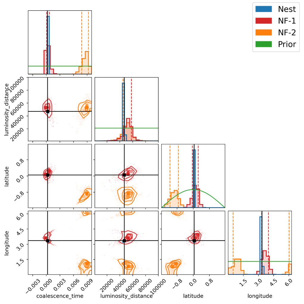
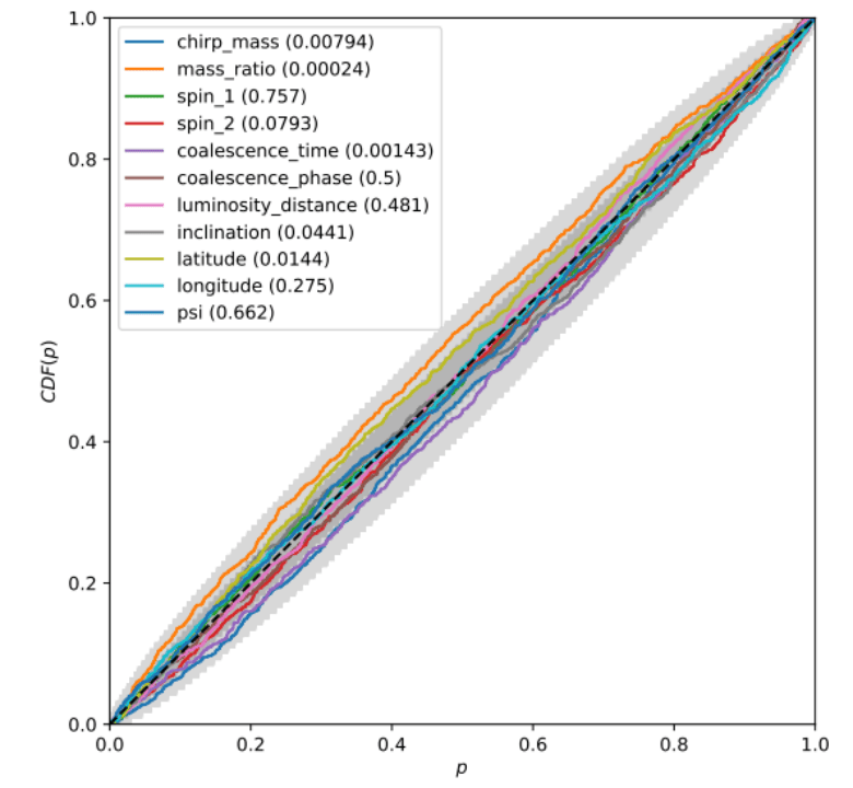
Results:
M. Du, B. Liang, HW, P. Xu, Z. Luo, Y. Wu. SCPMA 67, 230412 (2024).
-
Computational performance
-
10000 samples in 2.7 sec
-
-
Multimodality in extrinsic parameters
-
Unbiased estimation and confidence validation
Ongoing and Future Projects

| Pipeline | Targets | Programing Language (sampling method) | Comments |
|---|---|---|---|
|
GLASS (Littenberg&Cornish 2023) |
Noise, UCB, VGB, MBHB |
C / Python (TPMCMC / RJMCMC) | noise_mcmc+gb_mcmc+vb_mcmc+global_fit |
| Eryn | UCB | Python (TPMCMC / RJMCMC) | Mini code for UCB case |
| PyCBC-INFERENCE | MBHB | Python (?) | Unavailable |
| Bilby in Space / tBilby | MBHB / ? | ? / Python? (RJMCMC) | Unavailable |
| Strub et al. | UCB | ? (GP) | Unavailable / GPU-based |
| Zhang et al. (LZU) | UCB | ? (PSO) | MLP |
| Balrog | MBHB | ? |

(Sec.8.6 Red Book)
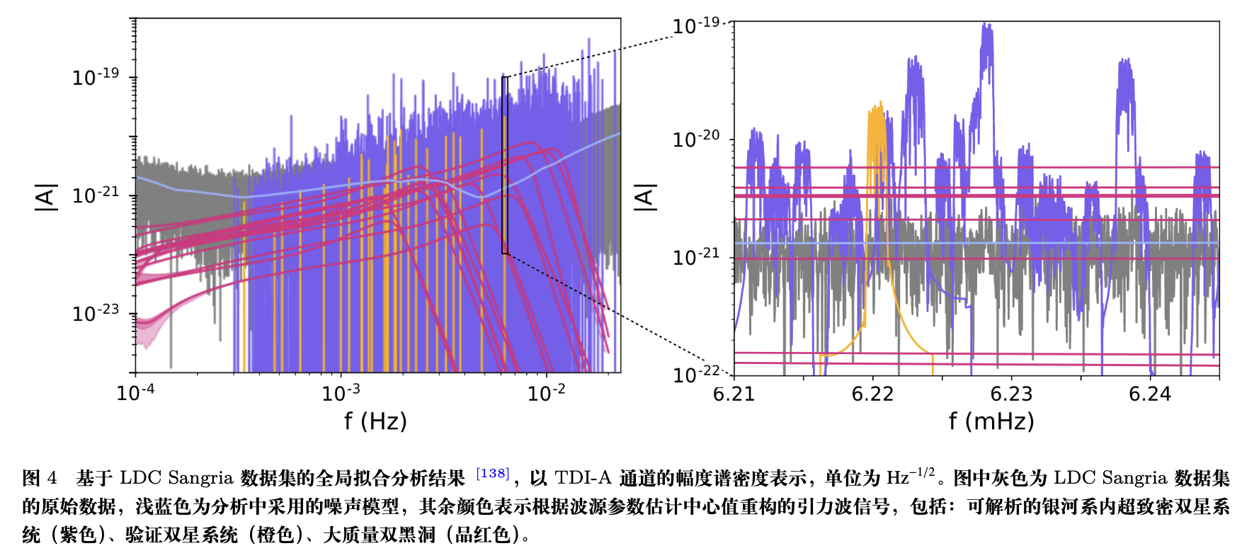
Global Fit
- The idea of the global fit method is to comprehensively model all astrophysical and instrumental features present in the space-borne gravitational wave data.
- This approach not only focuses on the signal from a single source, but attempts to capture the combined effects of all sources in the data, conducting a comprehensive analysis of the entire dataset to identify and model all potential signal and noise sources.
Technical challenges:
- High dimensional
- Highly correlated
- Multimodality
- Trans-dimensional
Text

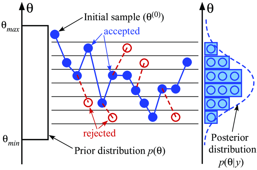
Ongoing and Future Projects
Neural density estimation
- Density fit for posterior distributions
- use the old posterior to form a proposal for the extended data.
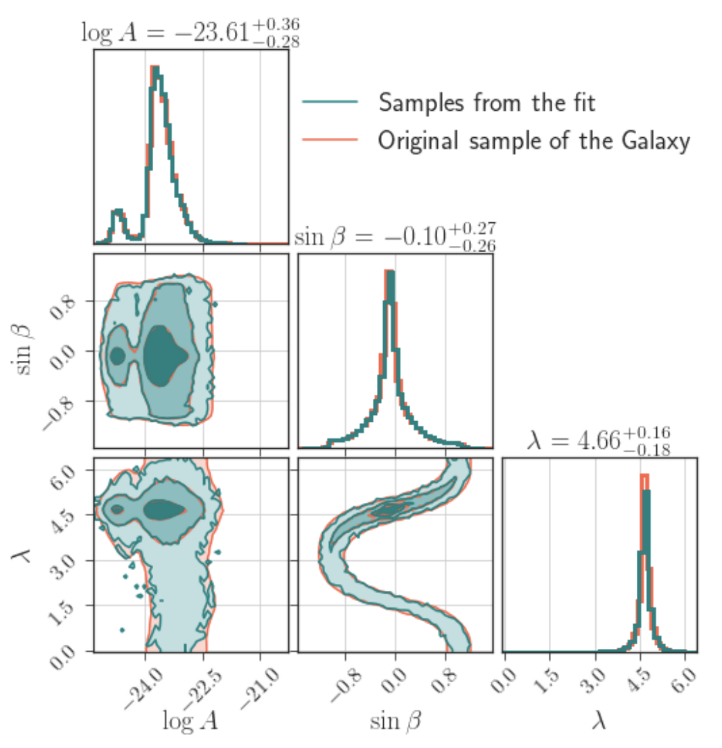
- Density fit for the Galaxy
- fitt a Galaxy model for joint distribution for \((A, \beta, \lambda)\).
- ...
Text


Ref:
- Ashton, G, and C Talbot. MNRAS 507, no. 2 (2021): 2037–51.
- Korsakova, N, et al. (2402.13701)
- Wouters, T, et al. (2404.11397)
Ongoing and Future Projects
Neural density estimation
- Density fit for posterior distributions
- use the old posterior to form a proposal for the extended data.
- Density fit for the Galaxy
- fitt a Galaxy model for joint distribution for \((A, \beta, \lambda)\).
- ...
Text


nflow


Ref:
- Ashton, G, and C Talbot. MNRAS 507, no. 2 (2021): 2037–51.
- Korsakova, N, et al. (2402.13701)
- Wouters, T, et al. (2404.11397)
Ongoing and Future Projects
Neural density estimation
- Density fit for posterior distributions
- use the old posterior to form a proposal for the extended data.
- Density fit for the Galaxy
- fitt a Galaxy model for joint distribution for \((A, \beta, \lambda)\).
- ...
Text


nflow


for _ in range(num_of_audiences):
    print('Thank you for your attention! 🙏')
This slide: https://slides.com/iphysresearch/2024may_cqupt