基于人工智能的引力波数据分析

王赫
2026/04/26
ICTP-AP, UCAS


hewang@ucas.ac.cn
-
Who Am I
— A quick intro and how I got into this field -
What Is Machine Learning?
— The basics and why it matters -
Deep Learning: When Machines Start to See and Think
— From neural networks to powerful representations -
Gravitational Waves Meet Machine Learning
— How ML is reshaping data analysis in GW astronomy -
Let’s Get Practical: Searching for Gravitational Waves
— A hands-on look at applying ML in real GW searches -
LLMs for Gravitational Waves: My Ongoing Work
— Towards automated and interpretable scientific discovery
Content

- AI for GW 的学习材料
- Normalizing Flows for PE
- History \(\rightarrow\) DINGO
- Current status (提及 DINGO for LISA, our SCPMA, our review)
- Mathematics of nflow
- Change of Variables
- 交叉熵与KL散度
- How to use conditional nflow for inference
- what is conditioner
- dataflow (SVD)
- 假设检验;IS;KS test
- verse Bayesian?
- What is SBI
- Let's coding!
- 引力波天文学
- 引力波数据分析
引力波天文学 · 数据处理
引力波天文学是个啥?
-
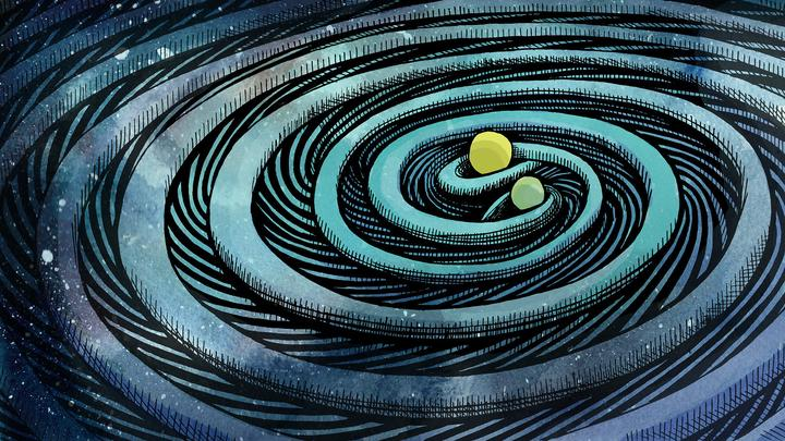
引力波是时空的涟漪。
-
大物体的引力扭曲空间和时间,或称为“时空”,就像保龄球在弹跳床上滚动时改变其形状一样。较小的物体因此会以不同的方式移动——就像弹跳床上朝向保龄球大小的凹陷螺旋而去的弹珠,而不是坐在平坦的表面上。

# AI for PE
引力波天文学是个啥?
-
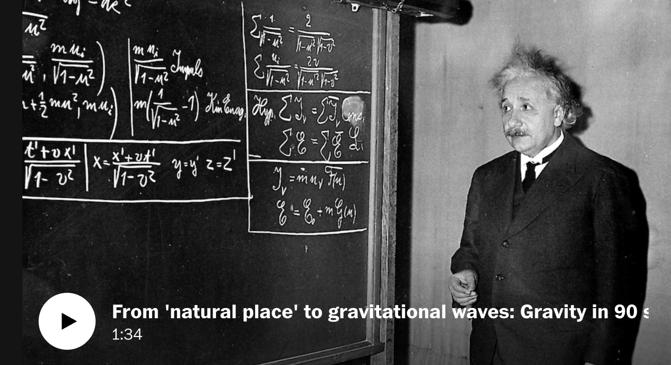
爱因斯坦于1916年提出广义相对论,并预言了引力波的存在
引力波是广义相对论中的一种强场效应-
2015年:首次实验探测到双黑洞并合引力波
-
2017年:首次双中子星多信使探测,开启多信使天文学时代
-
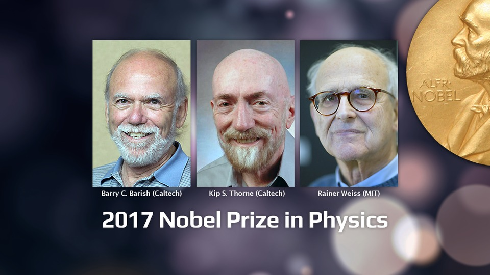
2017年:引力波探测成果被授予诺贝尔物理学奖
-
至今:发现了超过 90 个引力波事件
-
-
2024年:中国科学院大学加入地面引力波实验LIGO科学合作组织,成为LIGO目前在中国大陆地区的第二家成员单位。
-
未来规划:
-
2024-2025年:有希望探测到更多不同类型的引力波事件
-
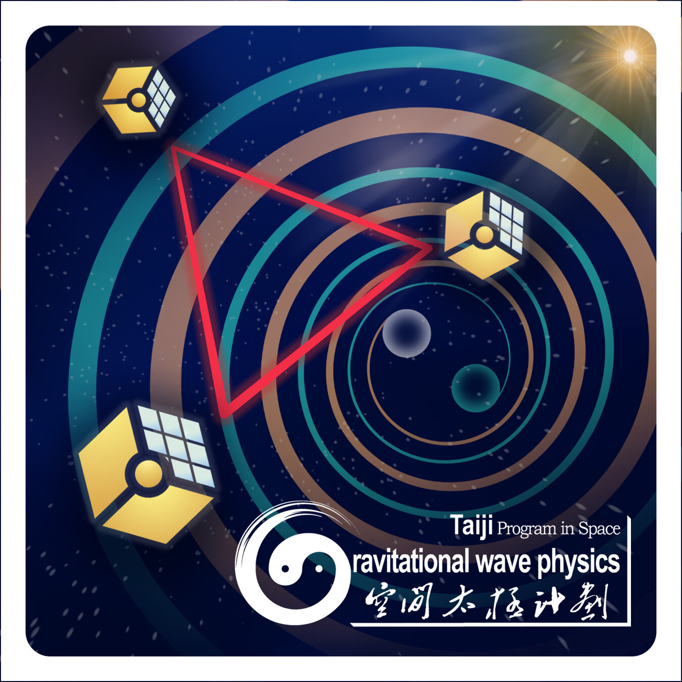
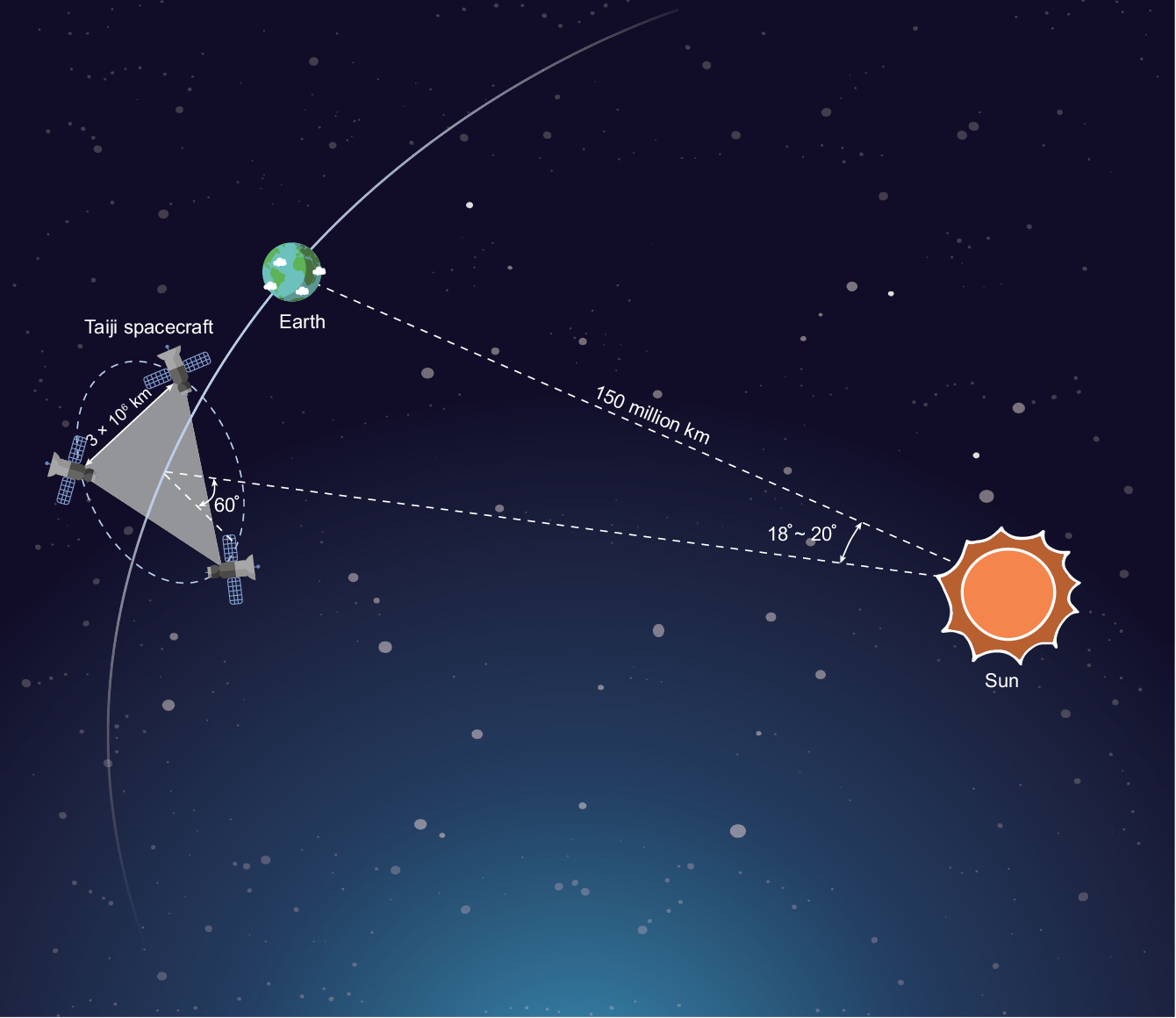
空间引力波探测计划 (LISA/Taiji/Tianqin) + XG (CE/ET)
-
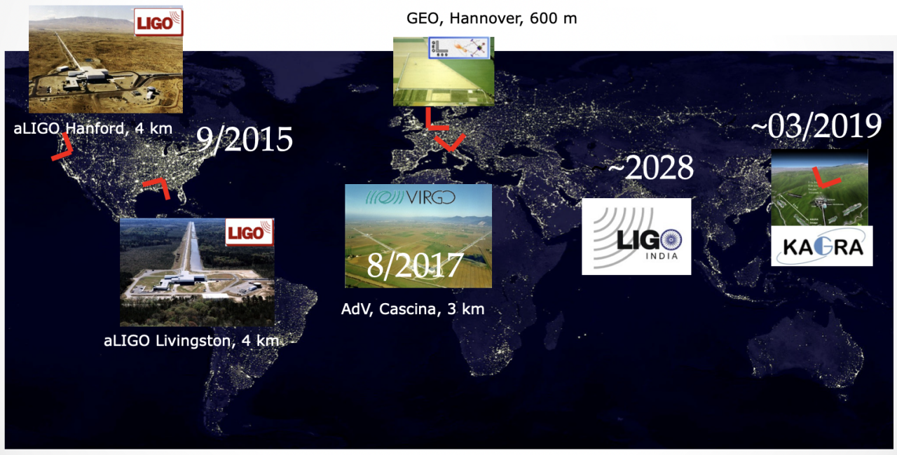
LIGO-VIRGO-KAGRA network

Gravitational waves generated by binary black holes system
GW detector
# AI for PE
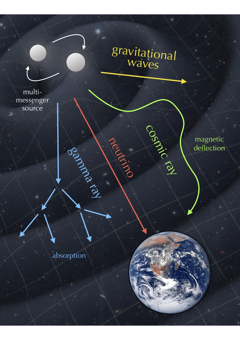
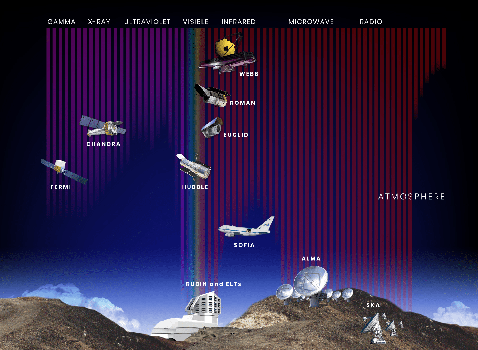
多信使天文学是个啥?
-
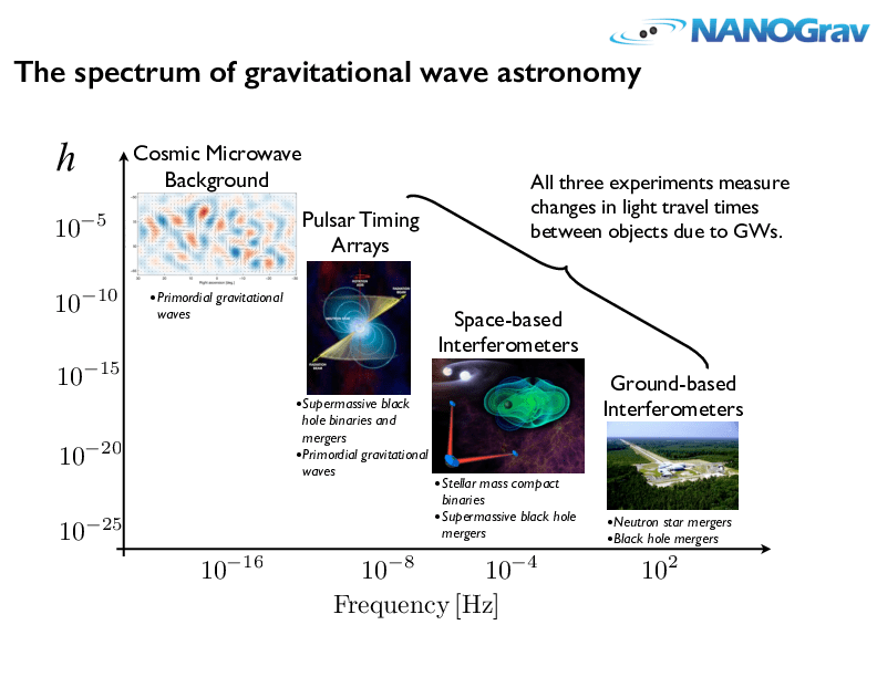
引力波探测打开了探索宇宙的新窗口
-
不同波源,频率跨越 20 个数量级,不同探测器
-
四种系外信使包括:电磁辐射、引力波、中微子,以及宇宙射线。
-
多信使天文学
# AI for PE
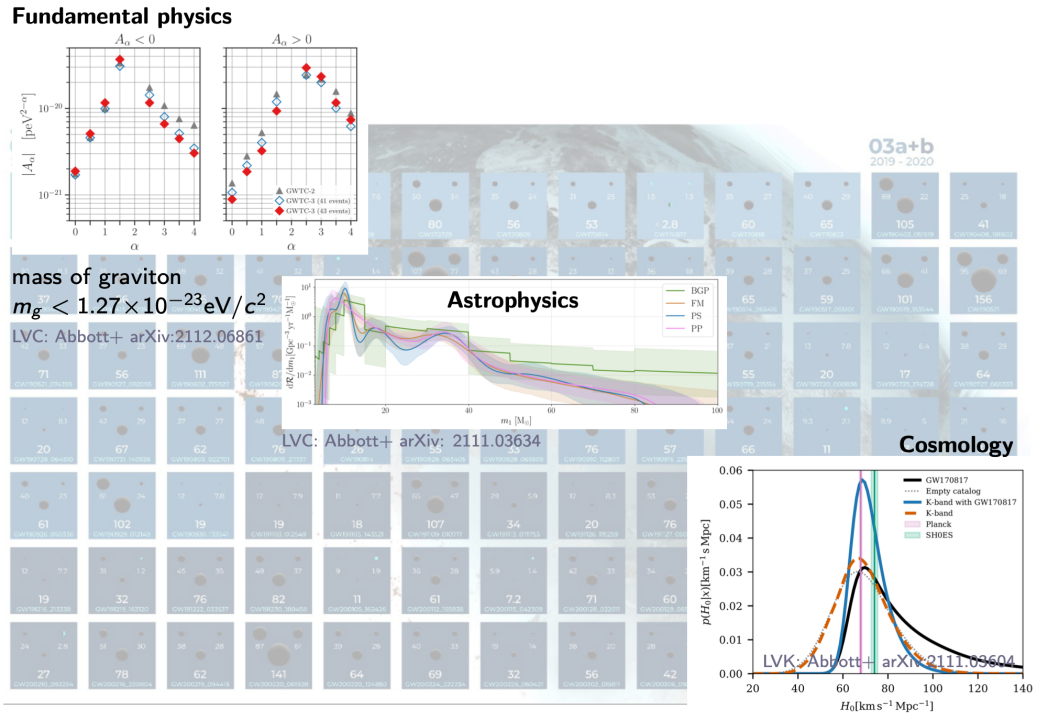
引力波天文学有啥科学意义?
- 基础理论的检验与修正
- 基础物理学
- 引力子是否有质量, 引力波的传播速度 ...
- 天体物理学
- 大质量恒星演化模型, 恒星级双黑洞的形成机制 ...
- 宇宙学
- 哈勃常数的测量, 暗能量 ...
- 基础物理学
- The current clouds over fundamental physics:
- 量子力学与广义相对论的统一
- 星系旋转曲线(暗物质)、宇宙加速膨胀(暗能量)
- 哈勃常数H0
- 中微子震荡和质量问题
- ...
-
# AI for PE
引力波天文学与数据分析
- 伯纳德·舒尔茨曾列出成功观测引力波的五条关键要素:
- 良好的探测器技术
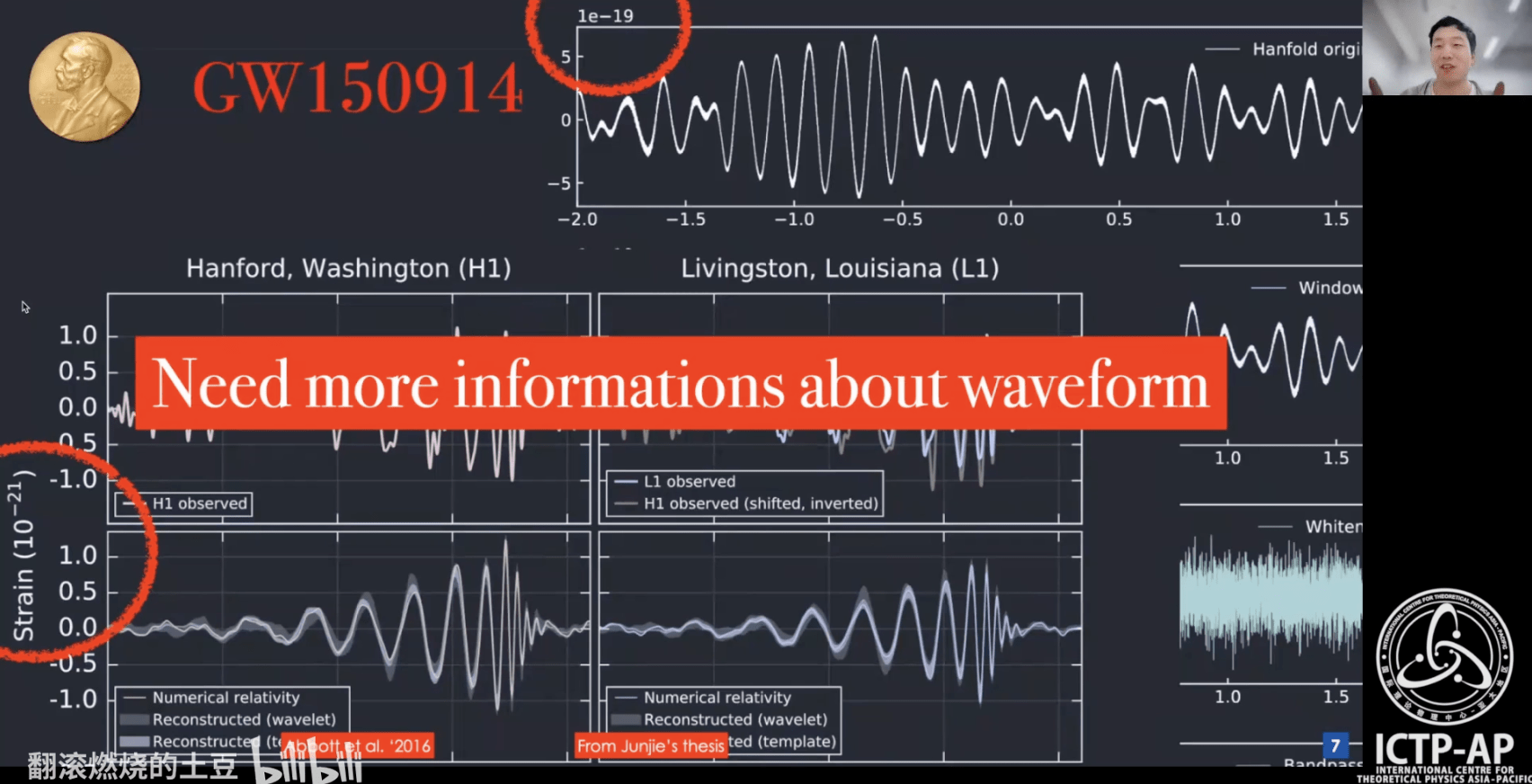
- 良好的波形模板
- 良好的数据分析方法和技术
- 多个独立探测器间的一致性观测
- 引力波天文学和电磁波天文学的一致性观测
DOI:10.1063/1.1629411
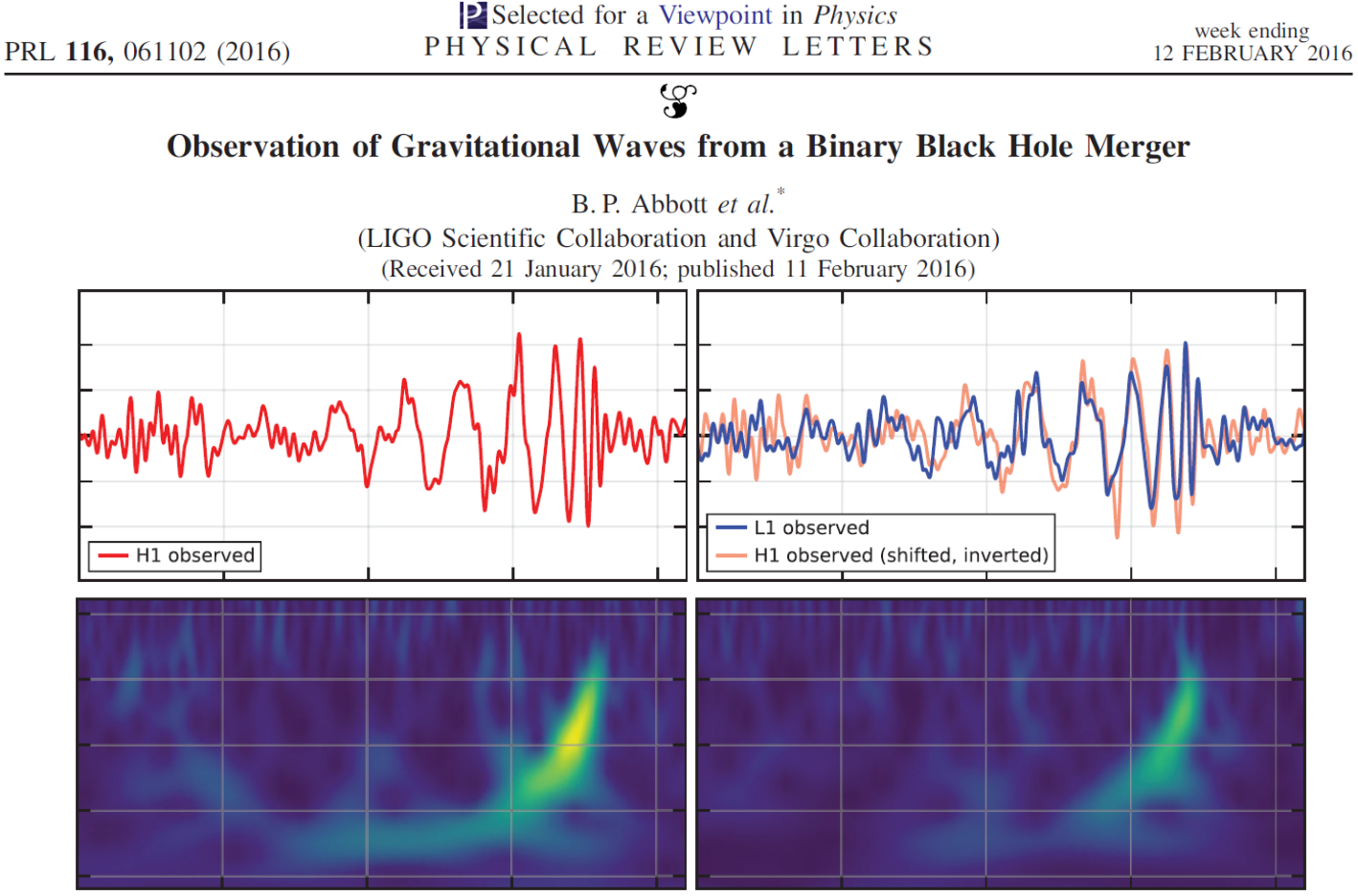
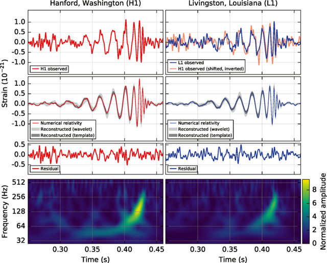
The first GW event of GW150914
LISA / Taiji project
LIGO-VIRGO-KAGRA
# AI for PE
引力波天文学与数据分析
GW Data Characteristics
LIGO-VIRGO-KAGRA
LISA Project
-
Noise: non-Gaussian and non-stationary
-
Signal challenges:
-
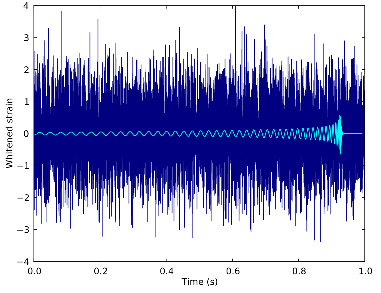
(Earth-based) A low signal-to-noise ratio (SNR) which is typically about 1/100 of the noise amplitude (-60 dB).
-
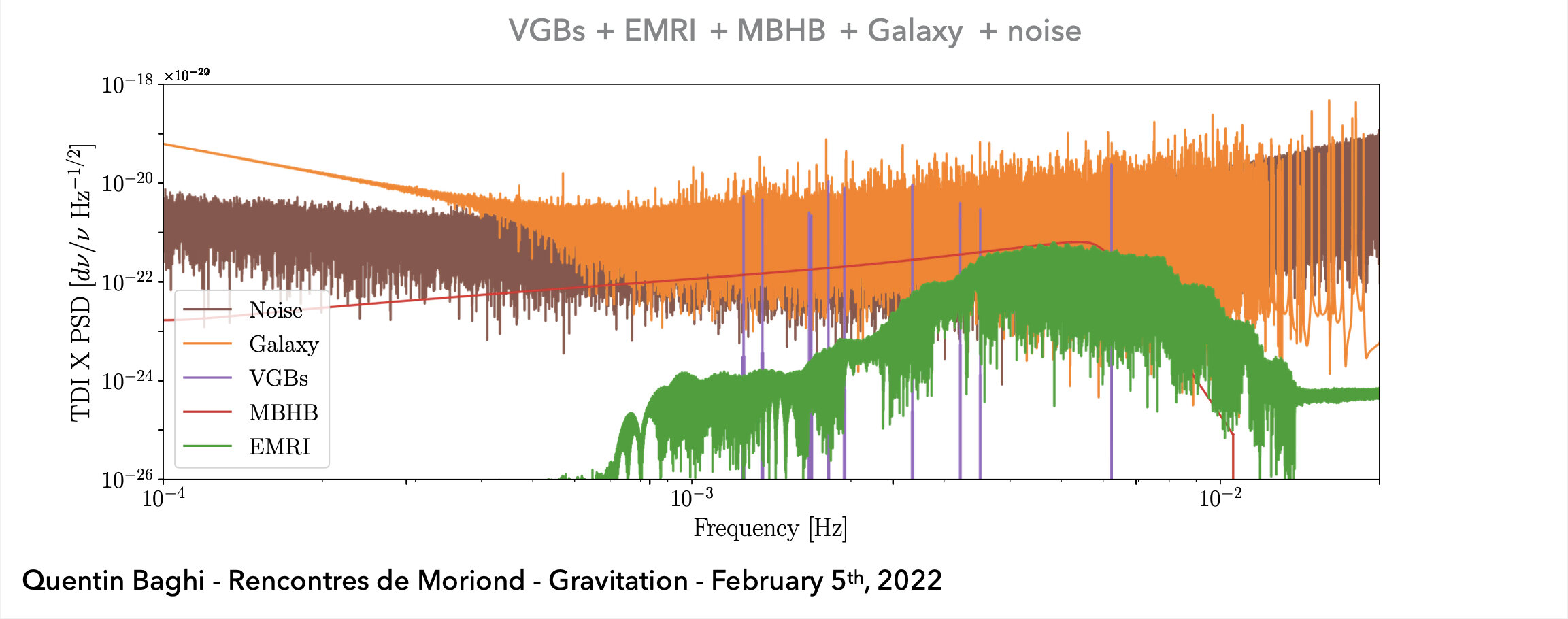
(Space-based) A superposition of all GW signals (e.g.: 104 of GBs, 10~102 of SMBHs, and 10~103 of EMRIs, etc.) received during the mission's observational run.
-

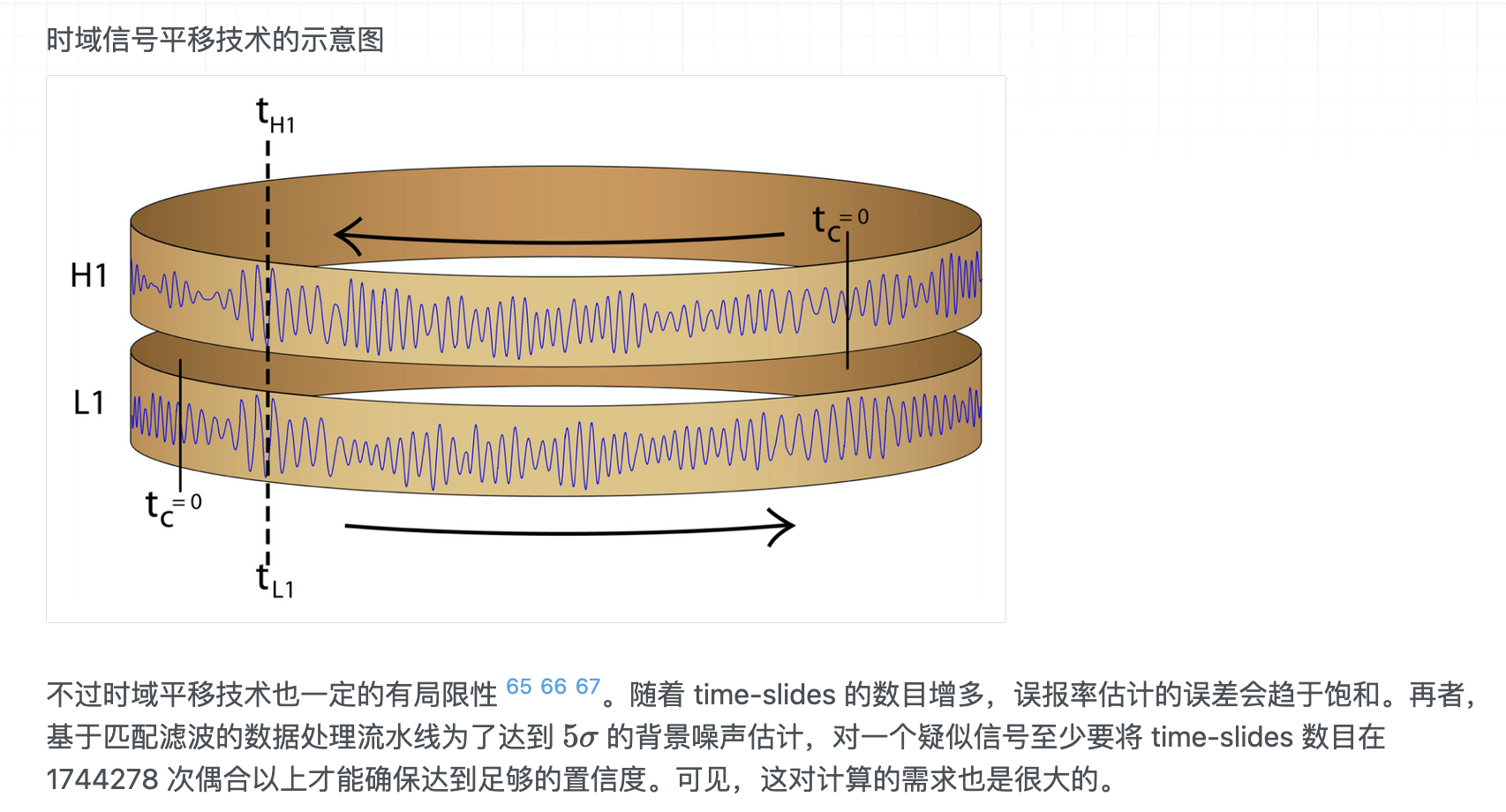
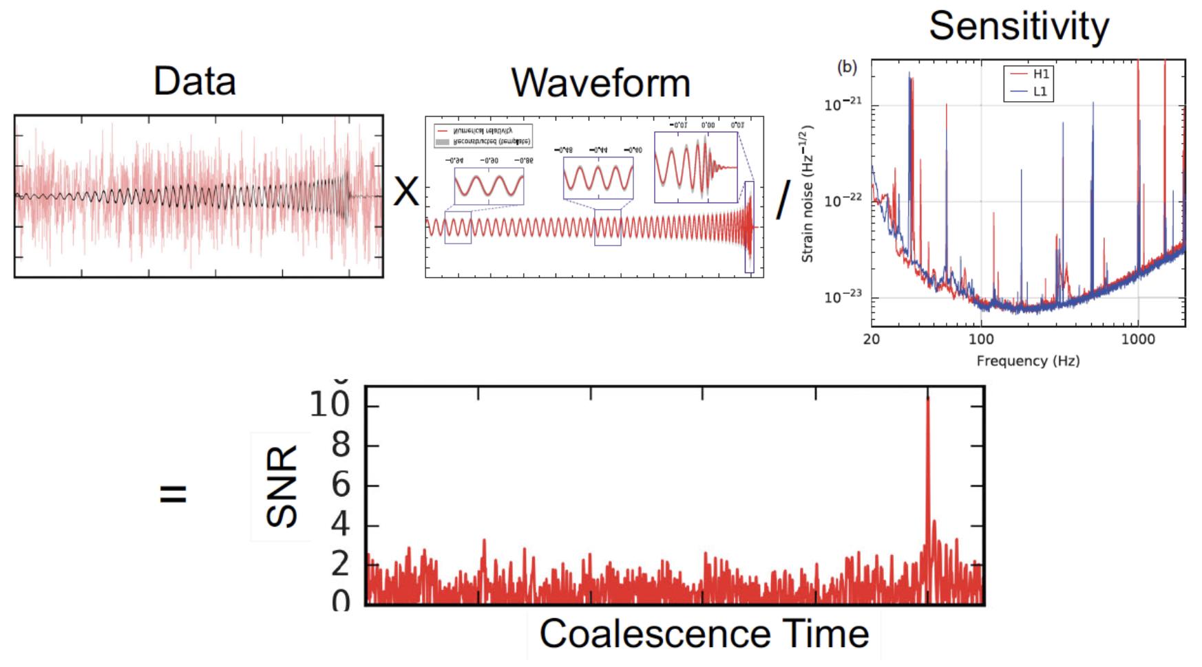
Matched Filtering Techniques (匹配滤波方法)
-
In Gaussian and stationary noise environments, the optimal linear algorithm for extracting weak signals
- Works by correlating a known signal model \(h(t)\) (template) with the data.
- Starting with data: \(d(t) = h(t) + n(t)\).
- Defining the matched-filtering SNR \(\rho(t)\):
\(\rho^2(t)\equiv\frac{1}{\langle h|h \rangle}|\langle d|h \rangle(t)|^2 \) , where
\(\langle d|h \rangle (t) = 4\int^\infty_0\frac{\tilde{d}(f)\tilde{h}^*(f)}{S_n(f)}e^{2\pi ift}df \) ,
\(\langle h|h \rangle = 4\int^\infty_0\frac{\tilde{h}(f)\tilde{h}^*(f)}{S_n(f)}df \),
\(S_n(f)\) is noise power spectral density (one-sided).
Statistical Approaches
Frequentist Testing:
- Make assumptions about signal and noise
- Write down the likelihood function
- Maximize parameters
- Define detection statistic
→ recover MF
Bayesian Testing:
- Start from same likelihood
- Define parameter priors
- Marginalize over parameters
- Often treated as Frequentist statistic
→ recover MF (for certain priors)
# AI for PE
引力波数据分析?

程序猿?
数据分析师?
运维工程师?

# AI for PE
引力波数据分析!

引力波物理科学家
数据科学家
人工智能
算法工程师

# AI for PE
真理的仲裁:从物理假说到算法验证
Everything begins with physics. Everything ends with algorithms.
- 理论家在自然的试卷上挥毫,实验家捕捉宇宙的笔触,而我们是那群在噪声中寻找真相的阅卷人。
Questions?
# AI for PE
- 经典书籍和专著
- 优秀课程资源
- 值得关注的公众号
- “引力波数据分析+人工智能” 入门学习资料推荐
人工智能技术自学材料推荐

机器学习与深度学习技术的学习材料
# GW: DL
书中例子多而形象,适合当做工具书
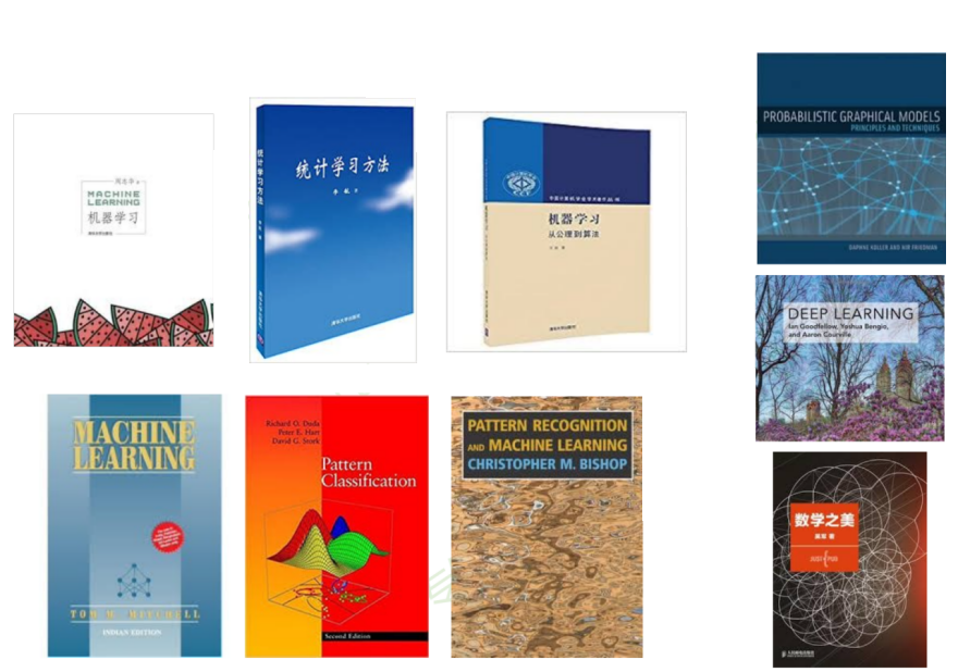
模型+策略+算法
(从概率角度)
机器学习
(公理化角度)
讲理论,不讲推导
经典,缺前沿
神书(从贝叶斯角度)
2k 多页,难啃,概率模型的角度出发
花书:DL 圣经
科普,培养直觉
机器学习与深度学习技术的学习材料
# GW: DL
工程角度,无需高等
数学背景
参数非参数
+频率贝叶
斯角度
统计角度
统计方法集大成的书
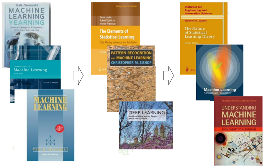
讲理论,
不会讲推导
贝叶斯角度
DL 应用角度
贝叶斯角度完整介绍
大量数学推导
机器学习与深度学习技术的学习材料
# GW: DL
优秀课程资源:
- CS231n(Stanford 李飞飞) / CS229 / CS230
- 吴恩达(ML / DL ...)
- 李宏毅(最佳中文课程,没有之一)
- 李沐-动手学深度学习(MXNet / PyTorch / TensorFlow)
- ... (多翻翻 Bilibili 就对了)
值得关注的公众号:
-
机器之心(顶流)
-
量子位(顶流)
-
新智元(顶流)
-
专知(偏学术)
-
微软亚洲研究院
-
将门创投
-
旷视研究院
-
DeepTech 深科技(麻省理工科技评论)
-
极市平台(技术分享)
- ...
-
爱可可-爱生活(微博、公众号、知乎、b站...)
-
陈光老师,北京邮电大学PRIS模式识别实验室
-
关于入门学习资料
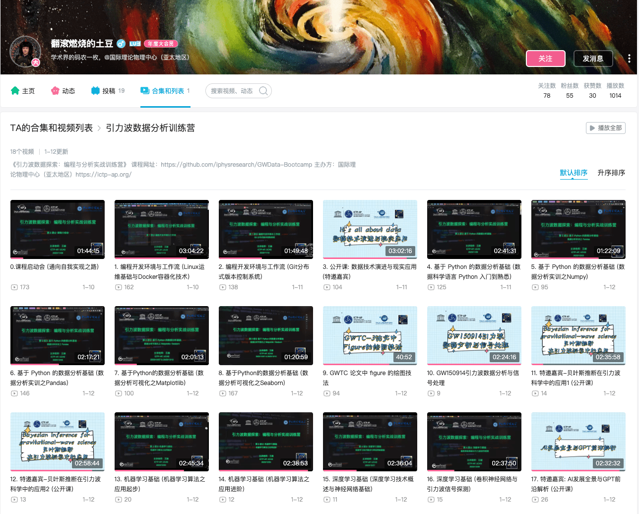
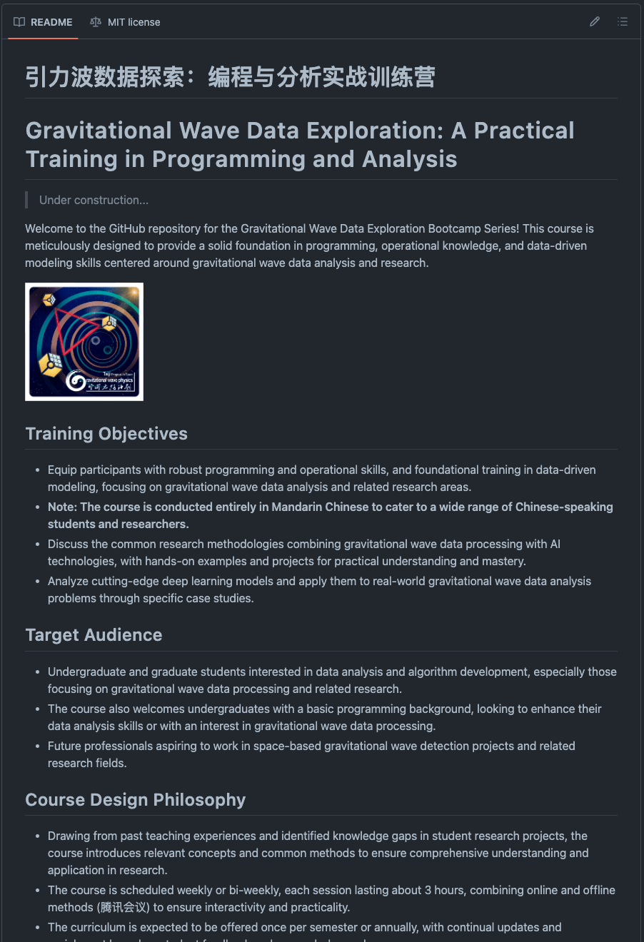

记得给课程 Star
《引力波数据探索:编程与分析实战训练营》(2023.10-2024.1)
- 第 0 部分:打鸡血!
- 通向自我实现之路
- 第 1 部分:编程开发环境与工作流
- 基础运维技术
- 容器化技术
- 实战项目:Python / Jupyter 开发环境搭建 + 远程连接 VS Code
- 实战项目:LALsuite / LISAcode 的源码编译 (optional)
- Git 分布式版本控制系统
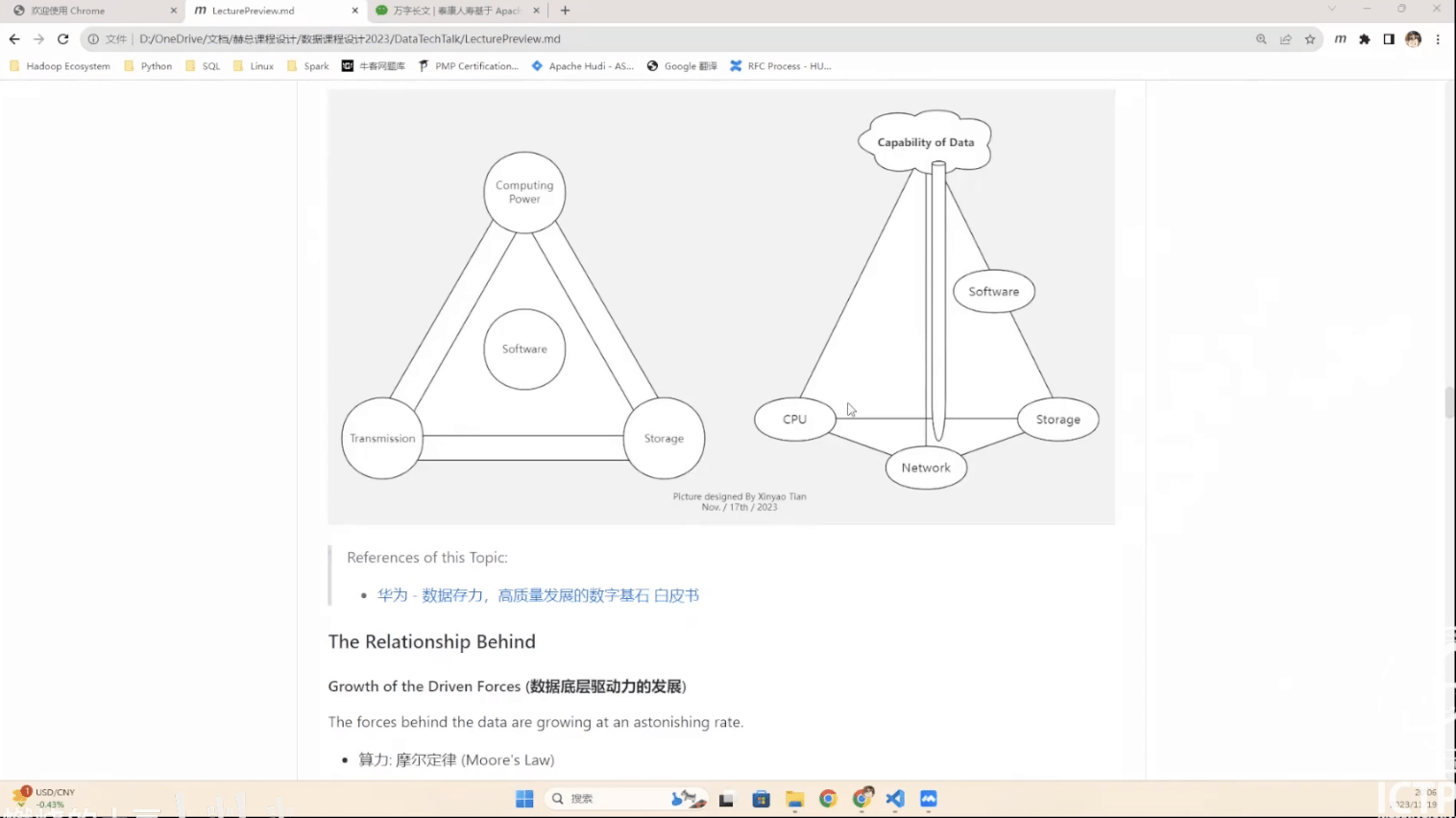
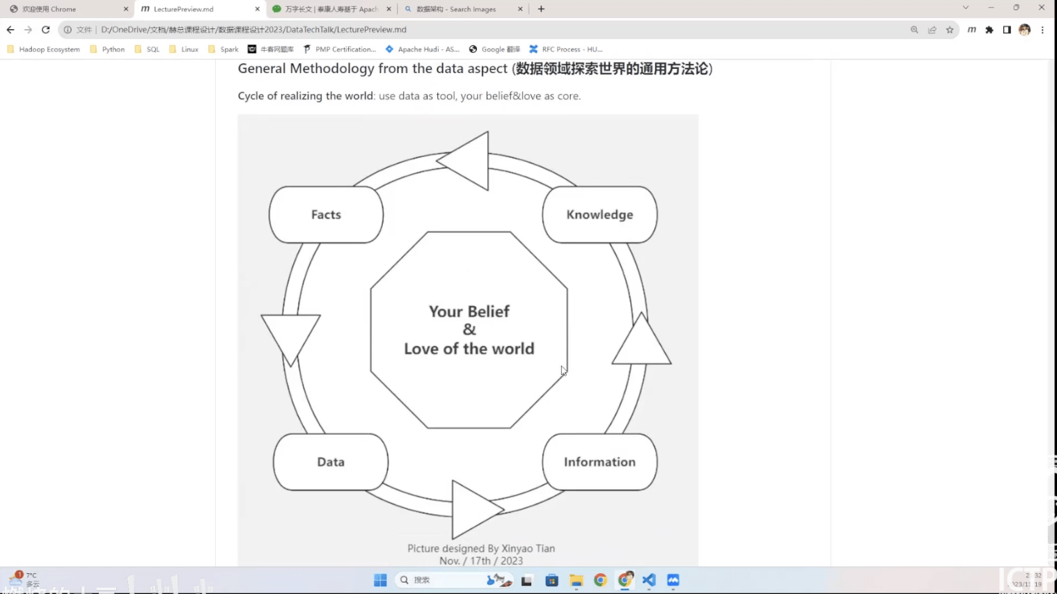
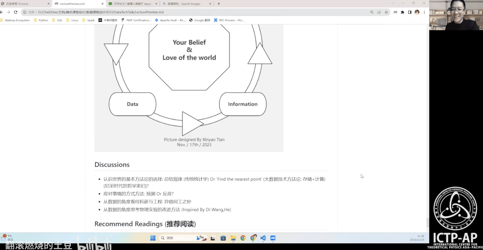
- 【公开课】数据技术演进与现实应用 (特邀嘉宾:田昕峣)
- 第 2 部分:基于 Python 的数据分析基础
- 数据科学语言 Python 从入门到熟悉
- 数据分析实训之 Numpy / Pandas
- 实战项目:GW Event Catalog 的探索性数据分析
- 实战项目:股票数据分析案例 (optional)
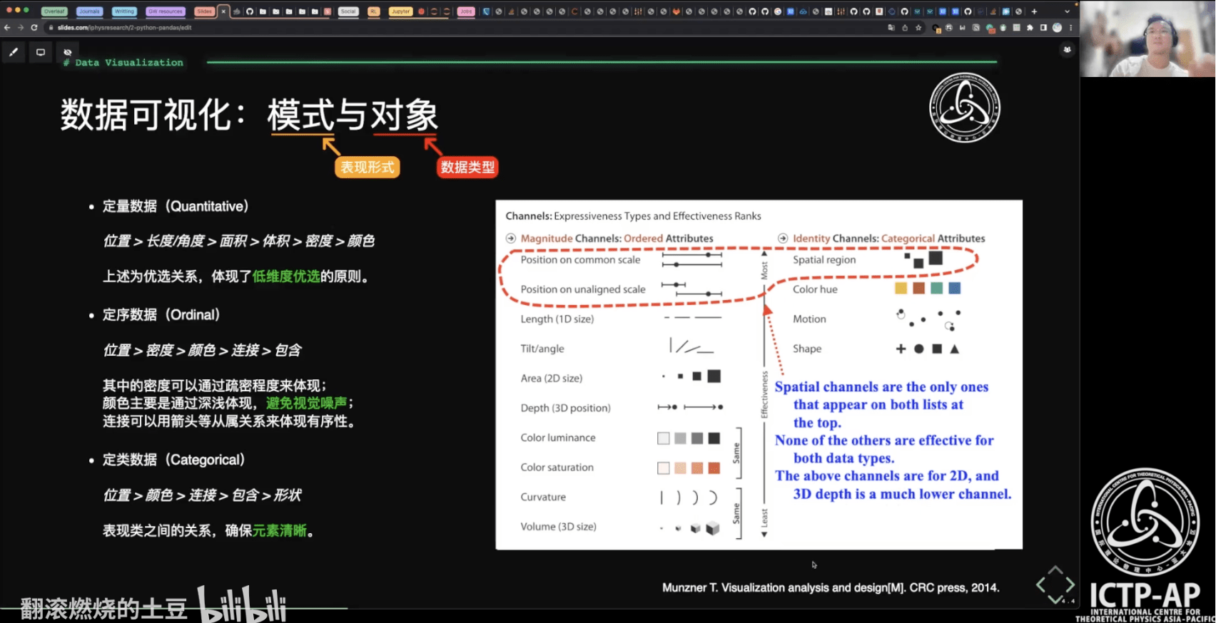
- 基于 Python 的数据可视化理论与实践之 Matplotlib / Seaborn
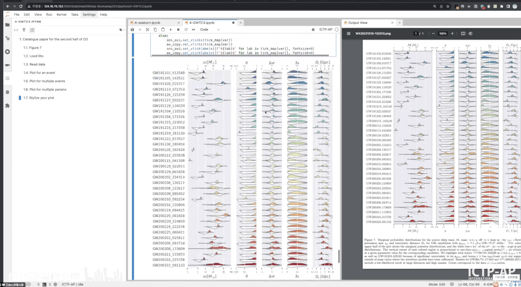
- 实战项目:GWTC 论文中的 Figures
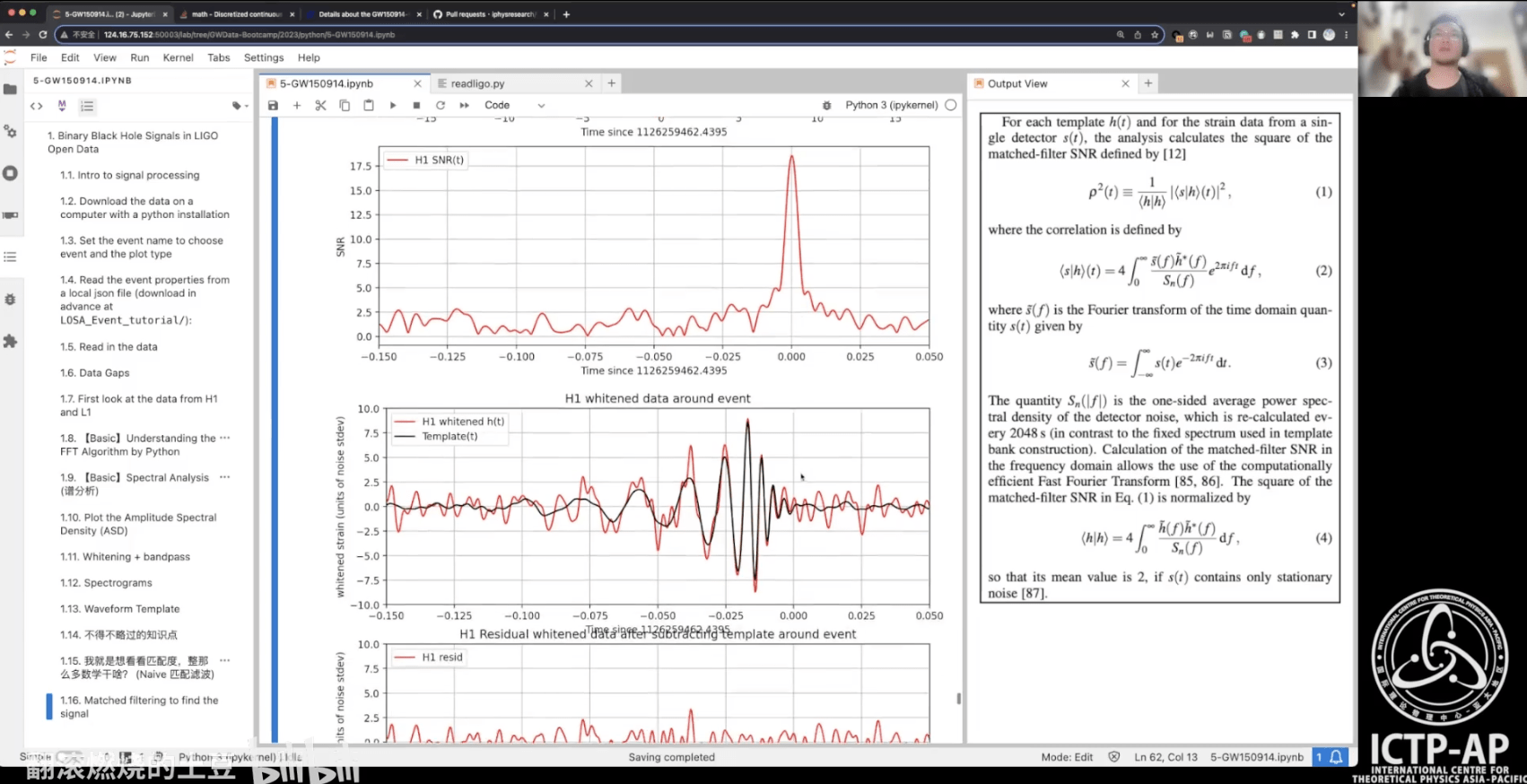
- 实战项目:针对 GW150914 信号处理与匹配滤波数据分析
- 【公开课】贝叶斯推断在引力波科学中的应用 (特邀嘉宾:赵俊杰)
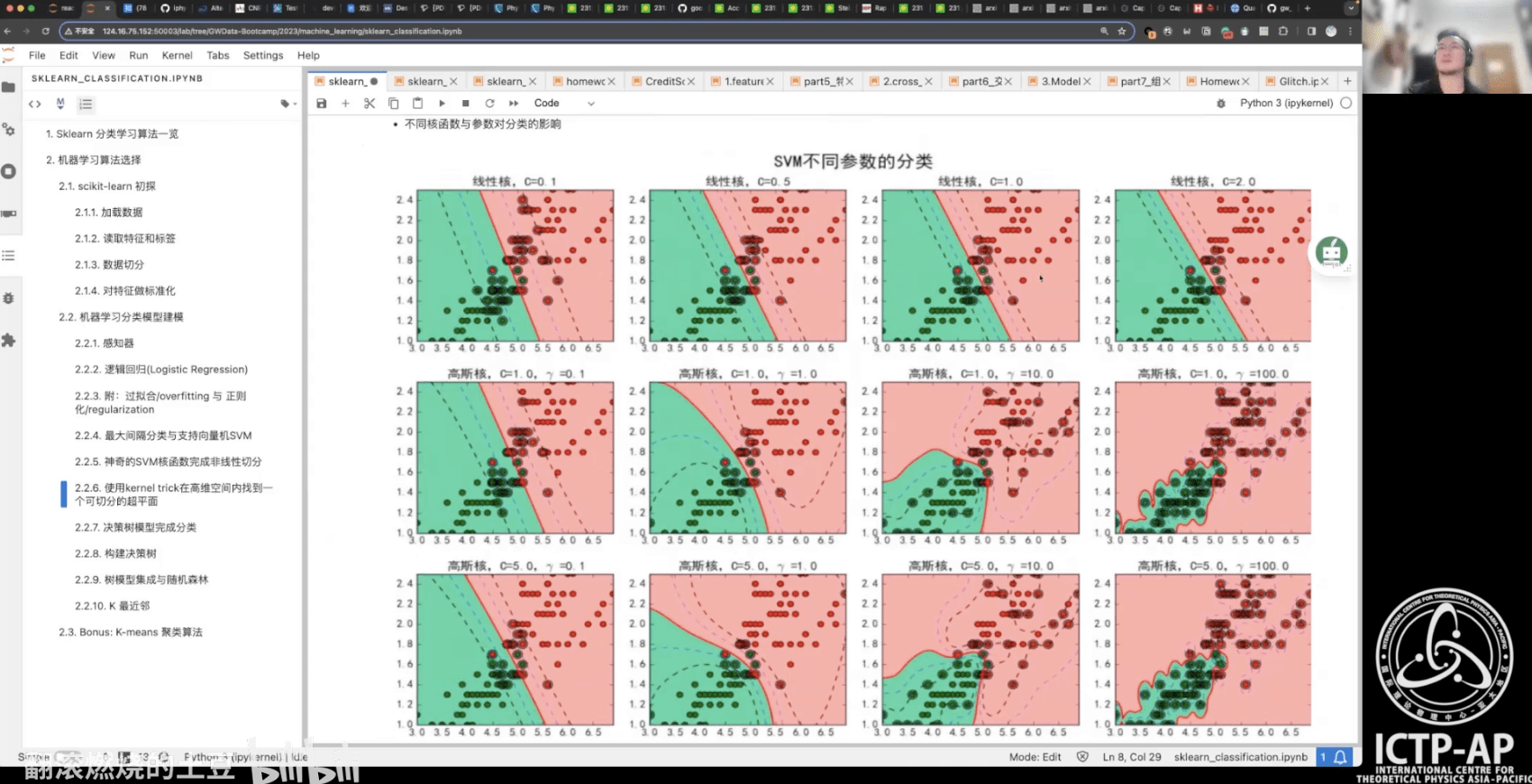
- 第 3 部分:机器学习基础
- 机器学习算法之应用起步
- 机器学习算法之应用进阶
- 实战项目:基于 LIGO 的 Glitch 元数据完成多分类任务
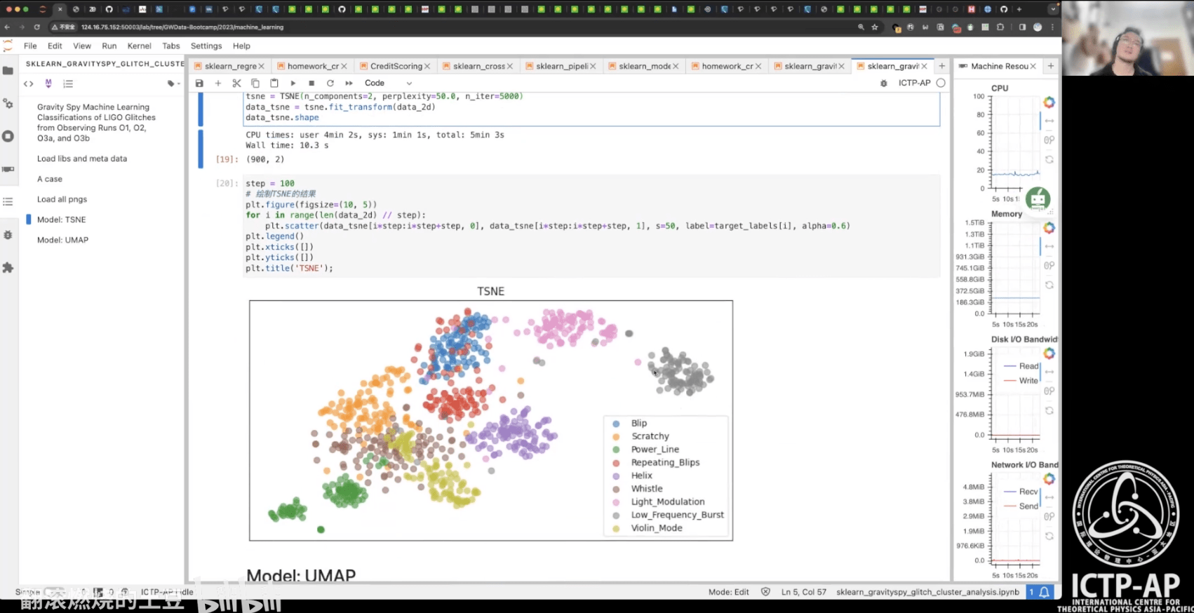
- 实战项目:基于 LIGO 的 Glitch 时频图数据实现聚类分析
- 第 4 部分:深度学习基础
- 深度学习技术概述与神经网络基础
- 实战项目:训练一个3层神经网络(手撸版)
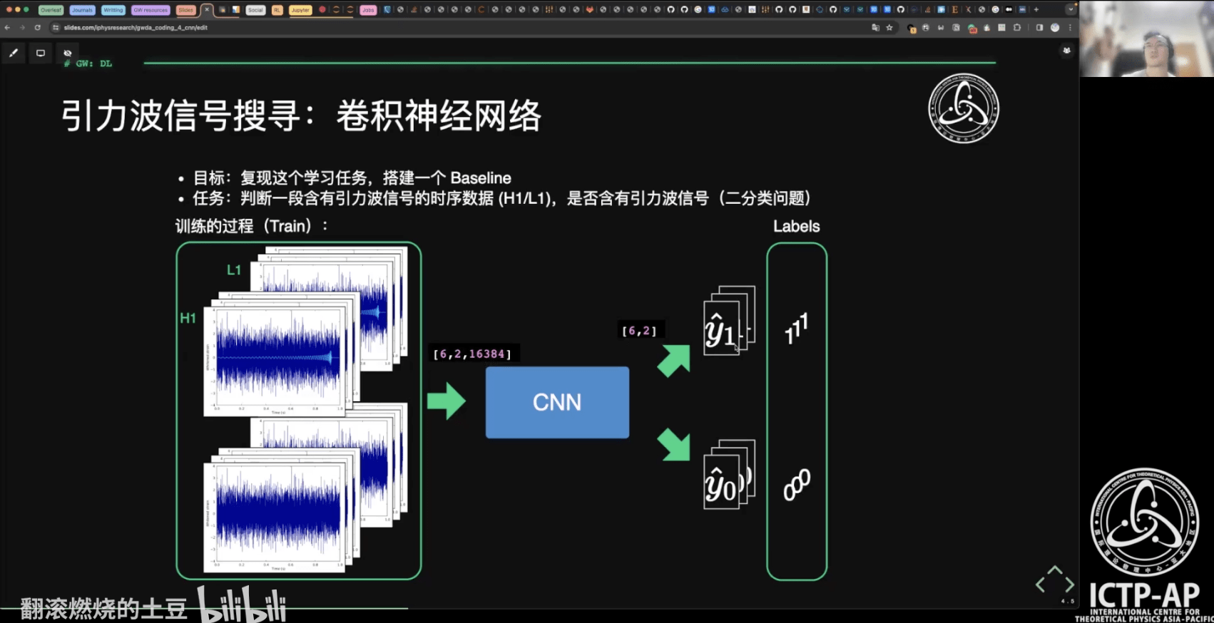
- 卷积神经网络与引力波信号探测
- 实战项目:使用 CNN 识别双黑洞系统引力波信号
- Kaggle数据科学竞赛 (黑客马拉松): Can you find the GW signals?
- 【公开课】AI发展全景与GPT前沿解析 (特邀嘉宾:高民权)
# AI for PE
关于入门学习资料
《引力波探测中关于深度学习数据分析的研究》(2020.6)
第一章 绪论
1.1 引言
1.2 多信使天文学
1.3 研究现状、机遇与挑战
1.4 本文研究的目标与框架
第二章 引力波探测和数据分析理论
2.1 引言
2.2 引力波探测技术
2.3 信号处理与数据分析方法
2.4 匹配滤波技术
第三章 深度学习的理论基础
3.1 引言
3.2 机器学习理论
3.3 深度神经网络
3.4 卷积神经网络
第四章 引力波探测中关于神经网络的可解释性研究
4.1 引言
4.2 神经网络的结构
4.3 数据集的制备和优化策略
4.4 引力波信号识别的泛化能力
4.5 引力波信号特征的可视化表示
4.6 引力波波形特征的灵敏度分析
第五章 卷积神经网络结构对引力波信号识别的性能研究
5.1 引言
5.2 引力波数据的制备和处理流程
5.3 引力波数据分析中信噪比的比较分析
5.4 卷积神经网络的超参数调优和性能比较
5.5 总结与结论
第六章 匹配滤波-卷积神经网络(MF-CNN)模型的应用研究
6.1 引言
6.2 时域中的匹配滤波
6.3 用于匹配滤波的卷积神经单元
6.4 匹配滤波-卷积神经网络(MF-CNN)模型的构造
6.5 搜寻疑似引力波信号的策略
6.6 数据准备与模型微调
6.7 真实 LIGO 引力波数据上的搜寻结果
6.8 总结与结论
第七章 总结与展望
附录
A. 采样定理与 Nyquist 频率
B. 关于功率谱密度性质的数学证明
C. 最大似然估计和交叉熵

# AI for PE
关于入门学习资料
《引力波开放数据》(2026.4.20-23)
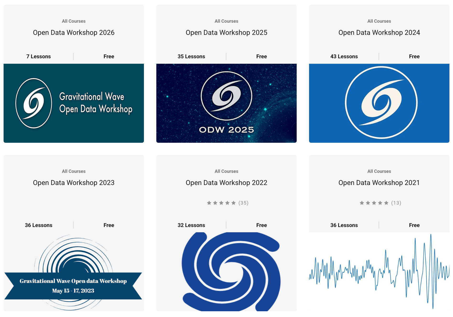
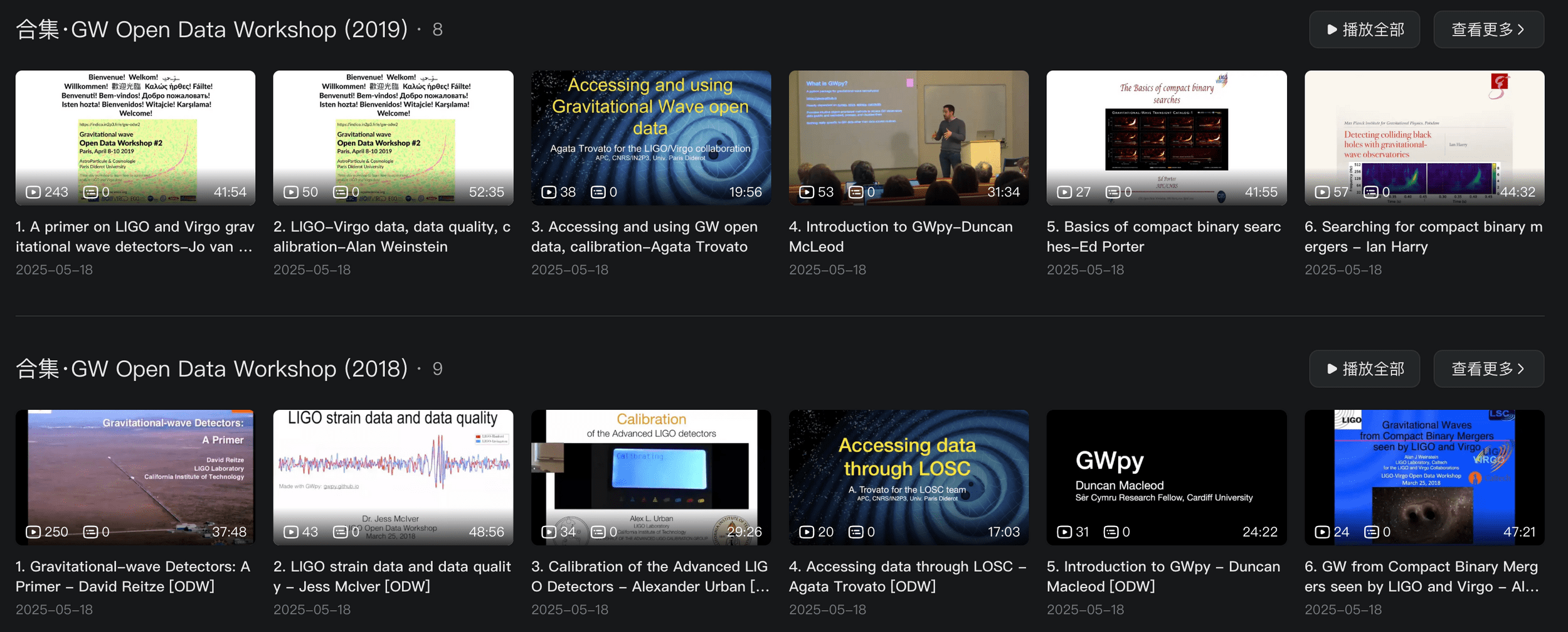
- 优秀ODW的往期视频:https://space.bilibili.com/76060243/lists
# AI for PE
关于入门学习资料
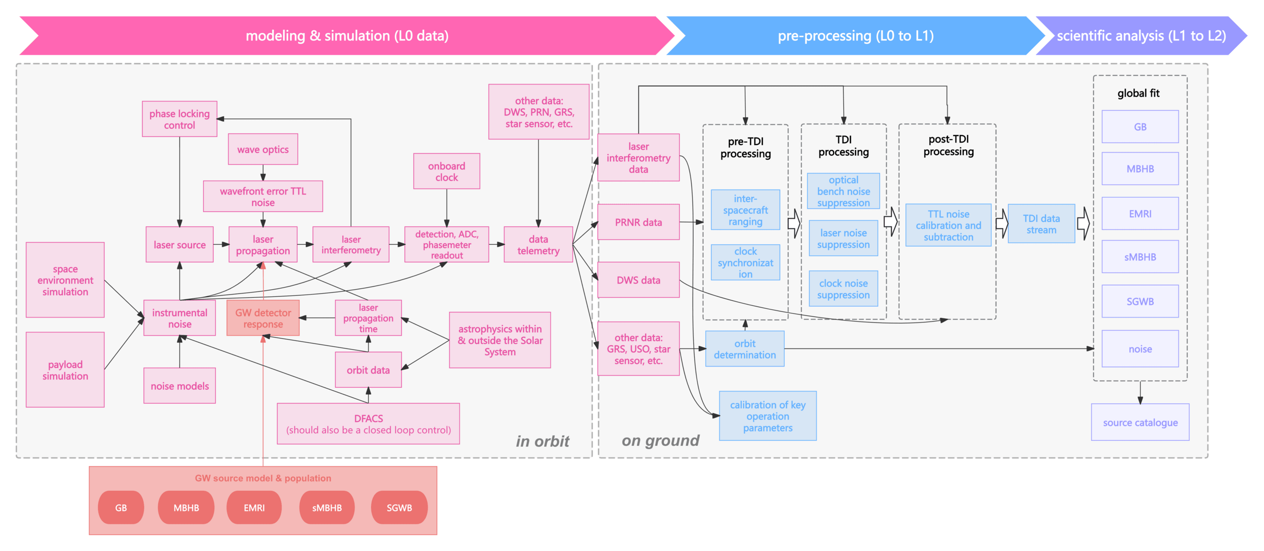
《空间引力波探测数据仿真及分析春季学习班》(2026.4.23-27)
- 空间引力波探测数据仿真及分析春季学习班将于 2026 年 4 月 23 日-27日
在中国科学院微小卫星创新研究院举办(线上+线下)。 - 课程大纲:空间引力波探测系统仿真(轨道动力学、无拖曳控制、光学、激光链路、引力波信号响应等)|引力波数据预处理(时间延迟干涉等)|空间引力波探测目标波源分析(大质量双黑洞、恒星级双黑洞、极端质量比旋近系统、银河系致密双星)|人工智能数据分析方法|引力波模型及引力波物理前沿。
- 官方链接:https://mp.weixin.qq.com/s/pwkZT51m9F-_OALb0ZrSQg
- 报名链接:https://v.wjx.cn/vm/PnPYjAJ.aspx
# AI for PE
- Flow-based inference
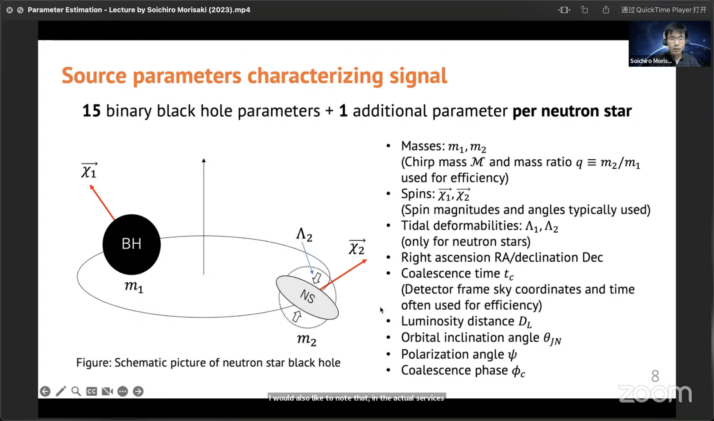
Parameter estimation

GW Parameter Estimation
# AI for PE
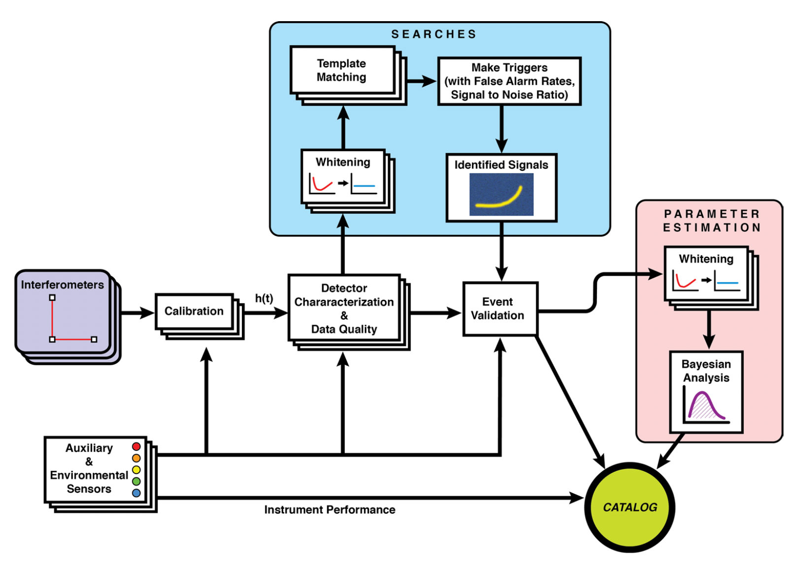
Data quality improvement
Credit: Marco Cavaglià
LIGO-Virgo-KAGRA data processing
GW waveform modeling
GW searches
Astrophsical interpretation of GW sources
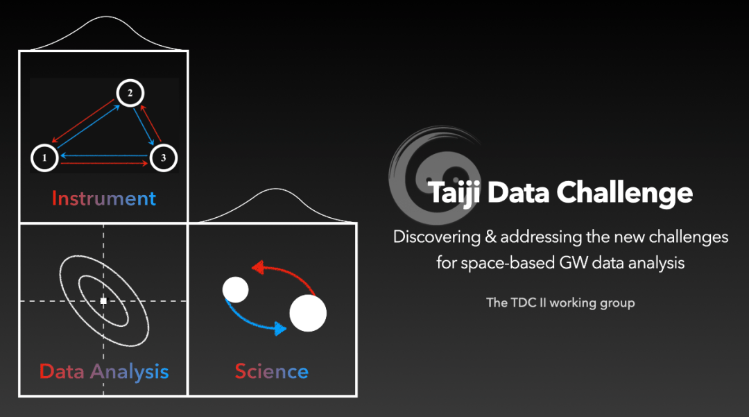
Space-based GW detection (Taiji program)
# AI for PE
Bayesian Inference
-
Traditional parameter estimation (PE) techniques rely on Bayesian analysis methods (posteriors + evidence)
-
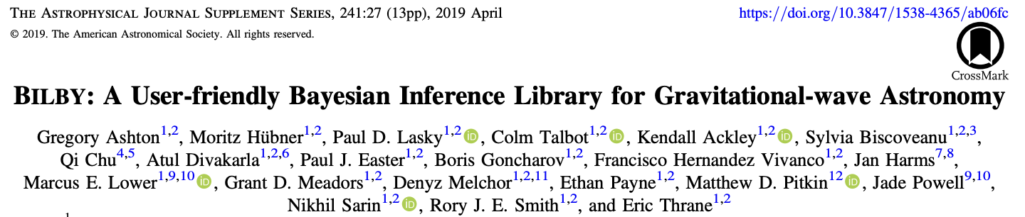
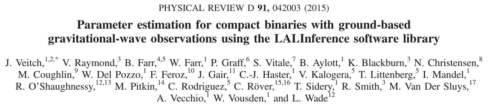
For CBC, LIGO-Virgo-KAGRA parameter estimation software:
-
Bilby / LALInference / PyCBC Inference / RIFT
-
- Computing the full 15-dimensional posterior distribution estimate is very time-consuming:
- Calculating likelihood function
- Template generation time-consuming
- Machine learning algorithms are expected to speed up! If it can be achieved in real-time, it will be more helpful for signal detection.
GW Parameter Estimation
Thrane, Eric, and Colm Talbot. “An Introduction to Bayesian Inference in Gravitational-Wave Astronomy: Parameter Estimation, Model Selection, and Hierarchical Models.” Publications of the Astronomical Society of Australia 36 (September 2019): e010. https://doi.org/10.1017/pasa.2019.2.
# AI for PE
GW Parameter Estimation via CVAE
- Deep Generative Models: Conditional Variational Autoencoder (CVAE)
- Noise Power Spectrum Based on Design Sensitivity, Gaussian Simulated Noise (Proof-of-principle studies)
- A complete 15-dimensional posterior probability distribution, taking about 1 second
An example: Posterior probability distribution of the complete 15-dimensional parameters
# AI for PE
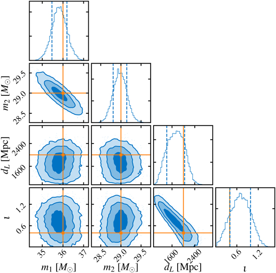
GW Parameter Estimation via NFlow
- Deep Generative Models: Normalizing Flow Models (Nflow)
- Noise Power Spectra Based on GW150914 Nearby Noise Estimation
- First Implementation of Full Posterior Parameter Estimation for Real Gravitational Wave Event GW150914
- 50,000 Posterior Samples in Approximately 8 Seconds
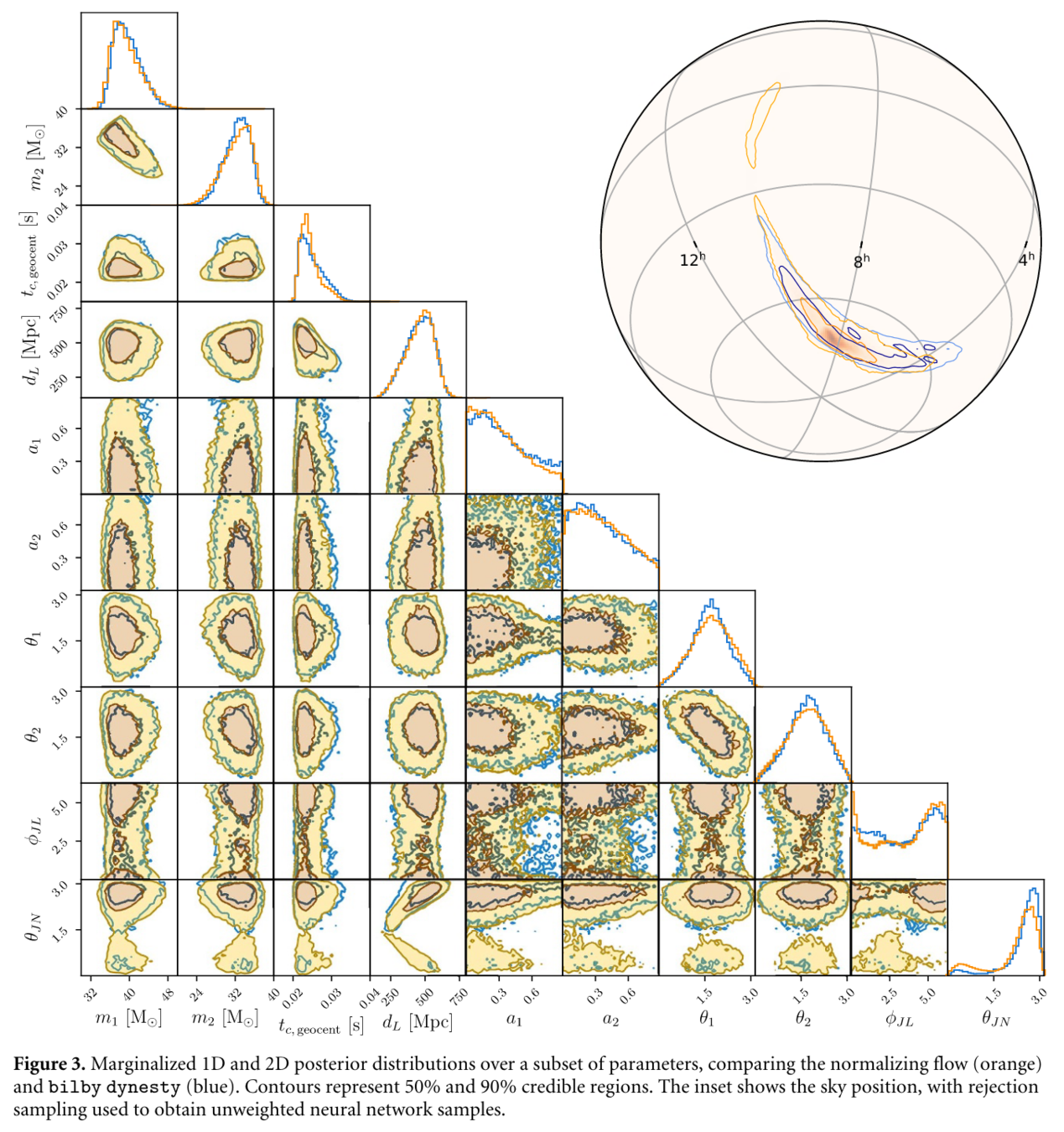
He Wang+, Big Data Mining and Analytics, 2021
# AI for PE
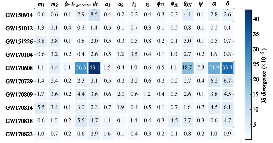
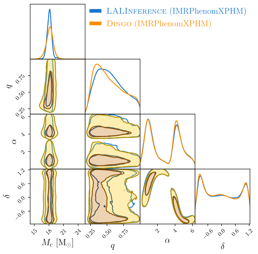
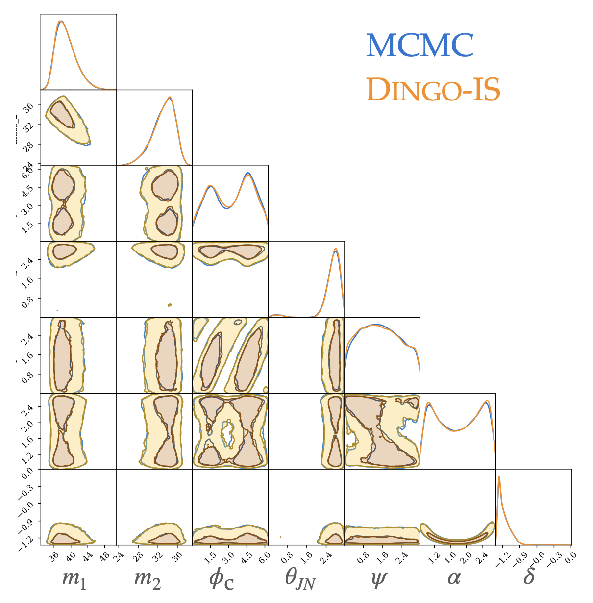
GW Parameter Estimation via NFlow
- 深度生成模型:归一化流模型 (Nflow)
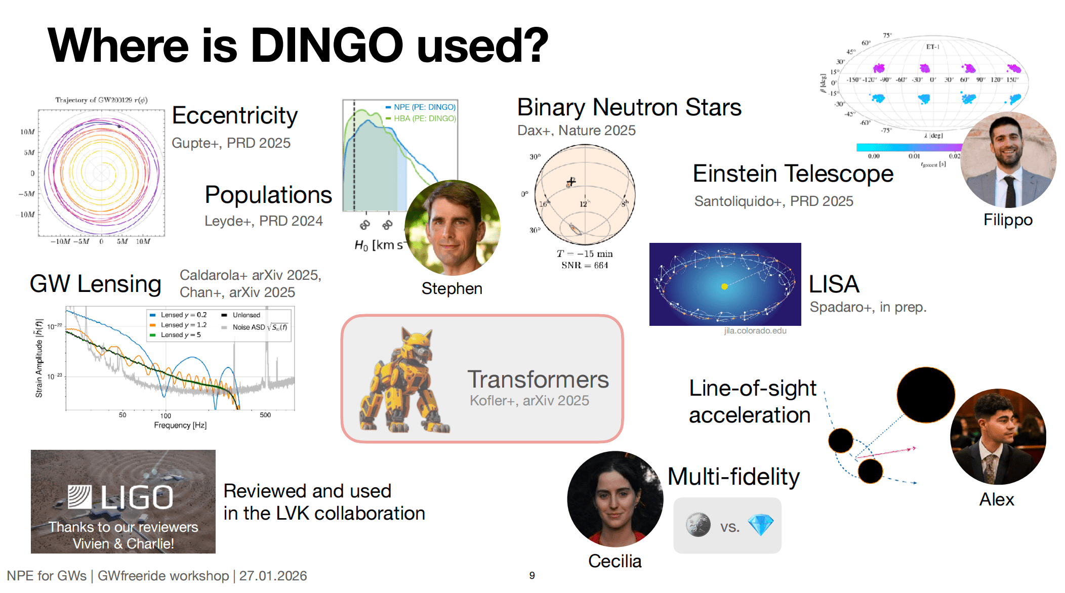
- DINGO (Deep INference for Gravitational wave Observations)
- 测试 GWTC-1 的 BBH 事件
- 耗时 < 1 min (≈ 20 s, IMRPhenomPv2)
- 开始为 O4 部署,有望成为新的引力波信号搜寻流水线
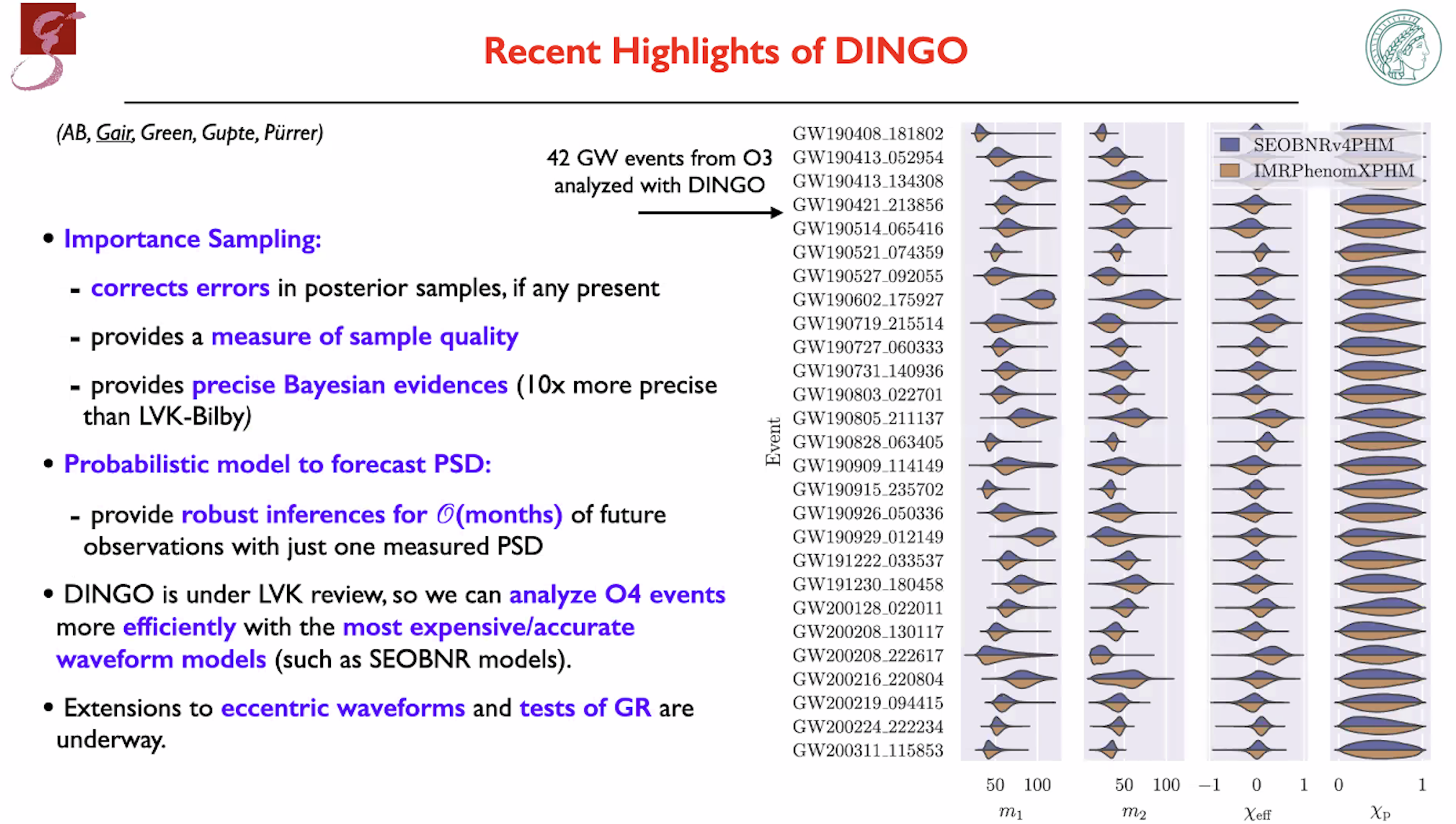
- DINGO-IS
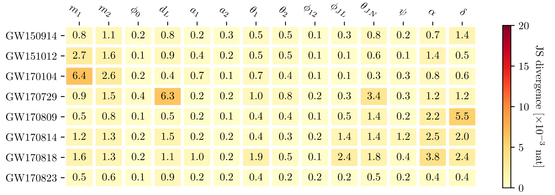
- 测试 GWTC-3 中 42 BBH 事件
- 耗时 ≲ 1 h (IMRPhenomXPHM),≈ 10 h (SEOBNRv4PHM, 64 CPU cores)
- 能够计算 evidence

# AI for PE
DINGO
-
進撃の DINGO in GW inference area.
-
2002.07656: 5D toy model [1] (PRD)
-
2008.03312: 15D binary black hole inference [1] (MLST)
-
2106.12594: Amortized inference and group-equivariant neural posterior estimation [2] (PRL)
-
2111.13139: Group-equivariant neural posterior estimation [2] (ICLR 2022)
-
2210.05686: +Importance sampling [2] (PRL)
-
2211.08801: Noise forecasting [2] (PRD)
-
2311.12093: Population studies [2] (PRD)
-
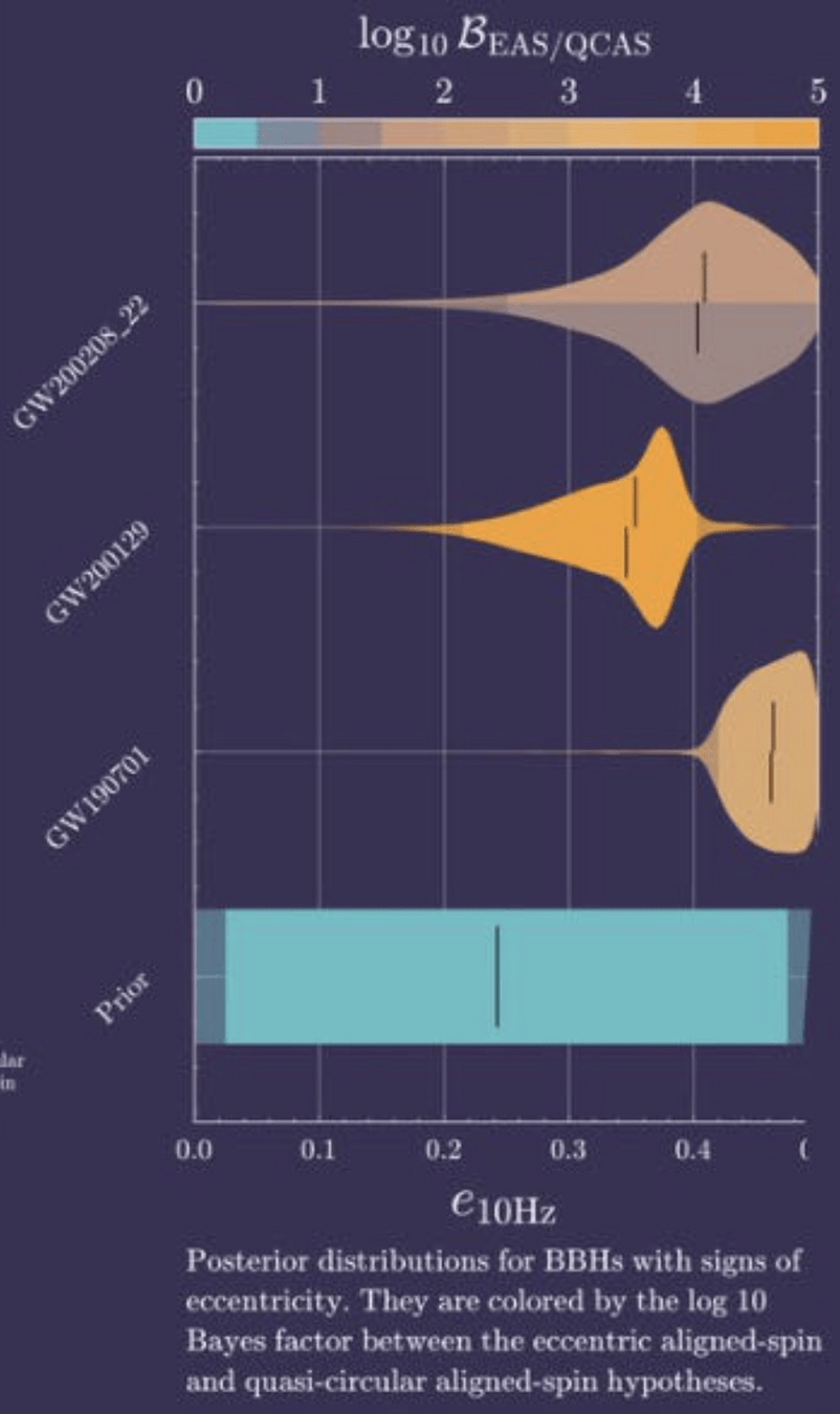
2404.14286: Find evidence for eccentric binaries. [2] (?)
-
2407.09602: BNS inference [2] (Nature)
-
2512.02968: +Transformer, (Dingo-T1) [3] (?)
-
2603.20431: For LISA [4] (?)
-
-
https://github.com/dingo-gw/dingo (2023.03)
-
https://github.com/dingo-gw/dingo-T1 (2025.11)
-
https://github.com/AliSword/dingo-lisa (2026.04)
-
https://github.com/stephengreen/gw-school-corfu-2023 (Tutorial)
-
https://github.com/annalena-k/tutorial-dingo-introduction (Tutorial)
- Some mathematics for NF
- Estimating GW parameters using NF
Normalizing Flows

# AI for PE
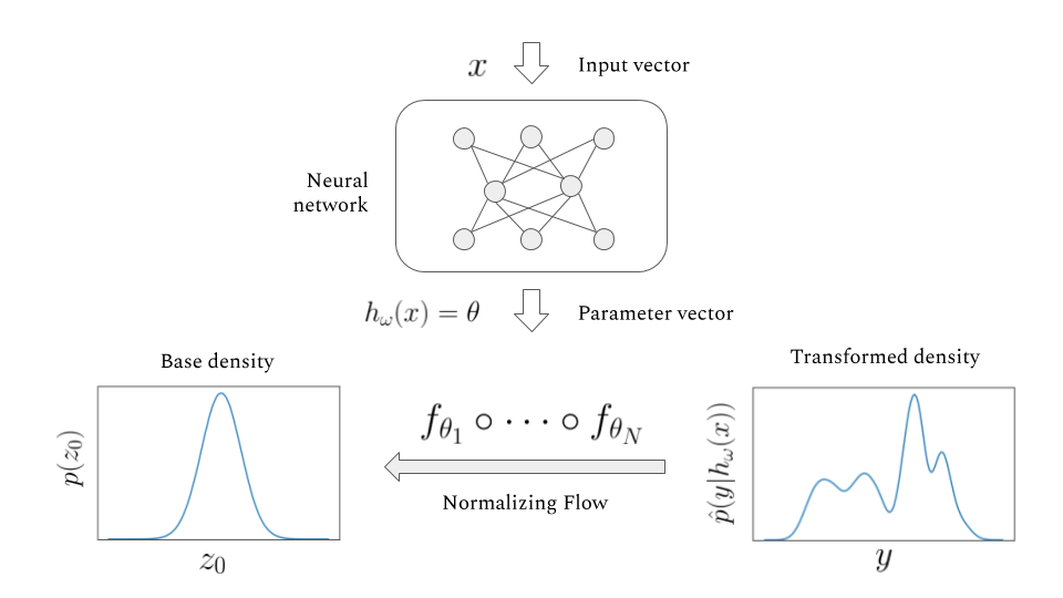
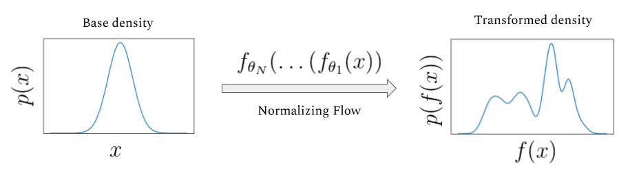
Normalizing Flows
The main idea of flow-based modeling is to express \(\mathbf{y}\in\mathbb{R}^D\) as a transformation \(T\) of a real vector \(\mathbf{z}\in\mathbb{R}^D\) sampled from \(p_{\mathrm{z}}(\mathbf{z})\):
(Based on 1912.02762)
Note: The invertible and differentiable transformation \(T\) and the base distribution \(p_{\mathrm{z}}(\mathbf{z})\) can have parameters \(\{\boldsymbol{\phi}, \boldsymbol{\psi}\}\) of their own, i.e. \( T_{{\phi}}\) and \(p_{\mathrm{z},\boldsymbol{\psi}}(\mathbf{z})\).
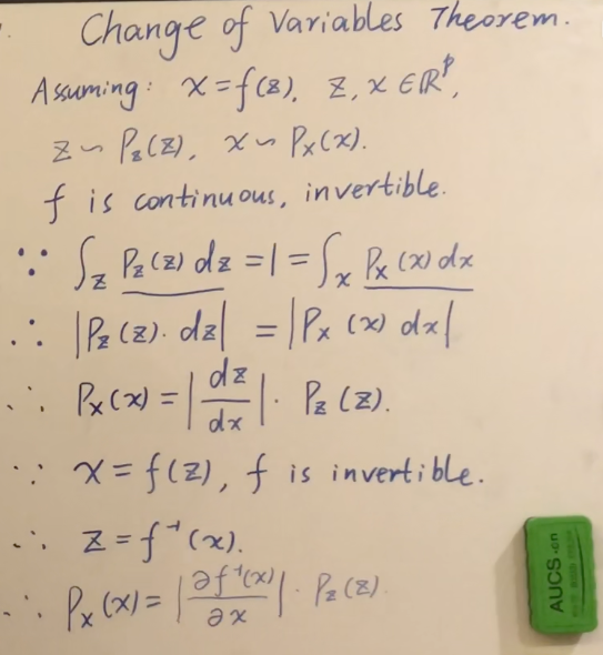
Change of Variables:
Equivalently,
The Jacobia \(J_{T}(\mathbf{u})\) is the \(D \times D\) matrix of all partial derivatives of \(T\) given by:
【【机器学习】白板推导系列(三十三) ~ 流模型(Flow based Model)】
base density
target density
# AI for PE
Normalizing Flows
(Based on 1912.02762)
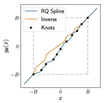
Rational Quadratic Neural Spline Flows
(RQ-NSF)
- Data: target data \(\mathbf{y}\in\mathbb{R}^{15}\) with condition data \(\mathbf{x}\).
- Task:
- Fitting a flow-based model \(p_{\mathrm{y}}(\mathbf{y} ; \boldsymbol{\theta})\) to a target distribution \(p_{\mathrm{y}}^{*}(\mathbf{y})\)
- by minimizing KL divergence with respect to the model’s parameters \(\boldsymbol{\theta}=\{\boldsymbol{\phi}, \boldsymbol{\psi}\}\),
- where \(\boldsymbol{\phi}\) are the parameters of \(T\) and \(\boldsymbol{\psi}\) are the parameters of \(p_{\mathrm{z}}(\mathbf{z})=\mathcal{N}(0,\mathbb{I})\).
- Loss function:
- Assuming we have a set of samples \(\left\{\mathbf{y}_{n}\right\}_{n=1}^{N}\sim p_{\mathrm{y}}^{*}(\mathbf{y})\),
Minimizing the above Monte Carlo approximation of the KL divergence is equivalent to fitting the flow-based model to the samples \(\left\{\mathbf{y}_{n}\right\}_{n=1}^{N}\) by maximum likelihood estimation.
base density
target density
# AI for PE
FYI:KL散度 vs 交叉熵
Objective:
- For each sample,
- Find the best \(\Theta\) that
在信息论中,可以通过某概率分布函数 \(p(x),x\in X\) 作为变量,定义一个关于 \(p(x)\) 的单调函数 \(h(x)\),称其为概率分布 \(p(x)\) 的信息量(measure of information): \(h(x) \equiv -\log p(x)\)
定义所有信息量的期望为随机变量 \(x\) 的 熵 (entropy):
若同一个随机变量 \(x\) 有两个独立的概率分布 \(p(x)\) 和 \(q(x)\),则可以定义这两个分布的相对熵 (relative entropy),也常称为 KL 散度 (Kullback-Leibler divergence),来衡量两个分布之间的差异:
可见 KL 越小,表示 \(p(x)\) 和 \(q(x)\) 两个分布越接近。上式中,我们已经定义了交叉熵 (cross entropy) 为
# AI for PE
FYI:KL散度 vs 交叉熵
Objective:
- For each sample,
- Find the best \(\Theta\) that
当对应到机器学习中最大似然估计方法时,训练集上的经验分布 \(\hat{p}_ \text{data}\) 和模型分布之间的差异程度可以用 KL 散度度量为:
由上式可知,等号右边第一项仅涉及数据的生成过程,和机器学习模型无关。这意味着当我们训练机器学习模型最小化 KL 散度时,我们只需要等价优化地最小化等号右边的第二项,即有
Recall:
由此可知,对于任何一个由负对数似然组成的代价函数都是定义在训练集上的经验分布和定义在模型上的概率分布之间的交叉熵。
# AI for PE
Normalizing Flows
base density
target density
e.g., Autoregressive Flow
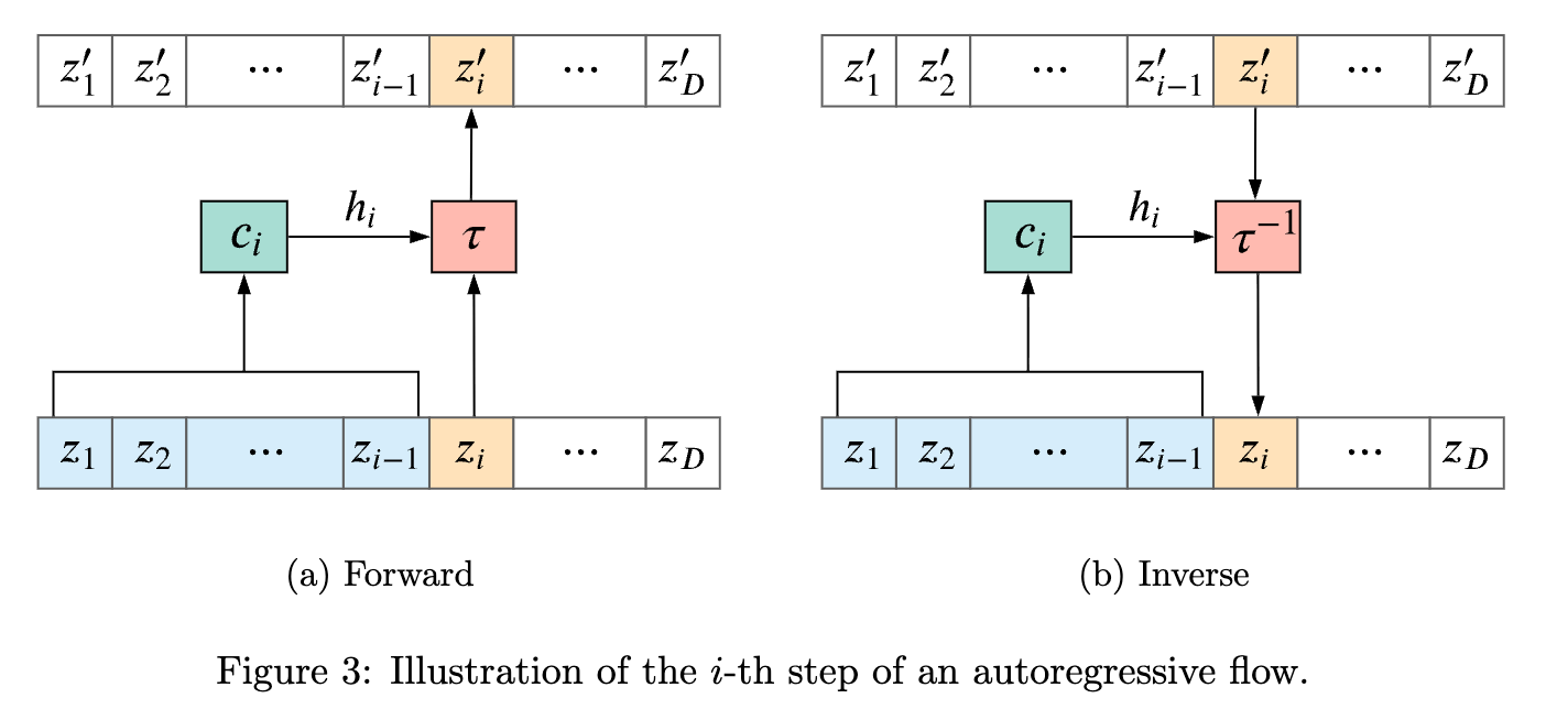
Autoregressive flow 的核心思想是按维度顺序逐个变换变量,每一步只依赖“已经生成/变换过的前面变量”,从而保证整体变换可逆且 Jacobian 易计算。
更具体地说:
- 在第 i 维,构造一个条件变换
\(z_i' = \tau(z_i;\, h_i), \quad h_i = c_i(z_1,\dots,z_{i-1})\)
也就是第 i 维的变换参数只由前 i-1 维决定(自回归结构)。
这里的 \(c_i\) 不是手写函数,而是一个神经网络。 - Forward(生成):从 \(z_1\) 到 \(z_D\) 顺序计算,每一步用已生成的前面变量作为条件。
- Inverse(求密度):可以逐维反解(因为每个 \(\tau\) 都是可逆的),同样是顺序的。
- 由于这种“下三角依赖结构”,Jacobian 是三角矩阵,行列式就是对角项乘积,因此 log-det 很容易计算。
一句话总结:
👉 autoregressive flow = “按顺序逐维做条件可逆变换”,用因果结构换取可逆性 + 高效概率计算。
# AI for PE
Normalizing Flows
base density
target density
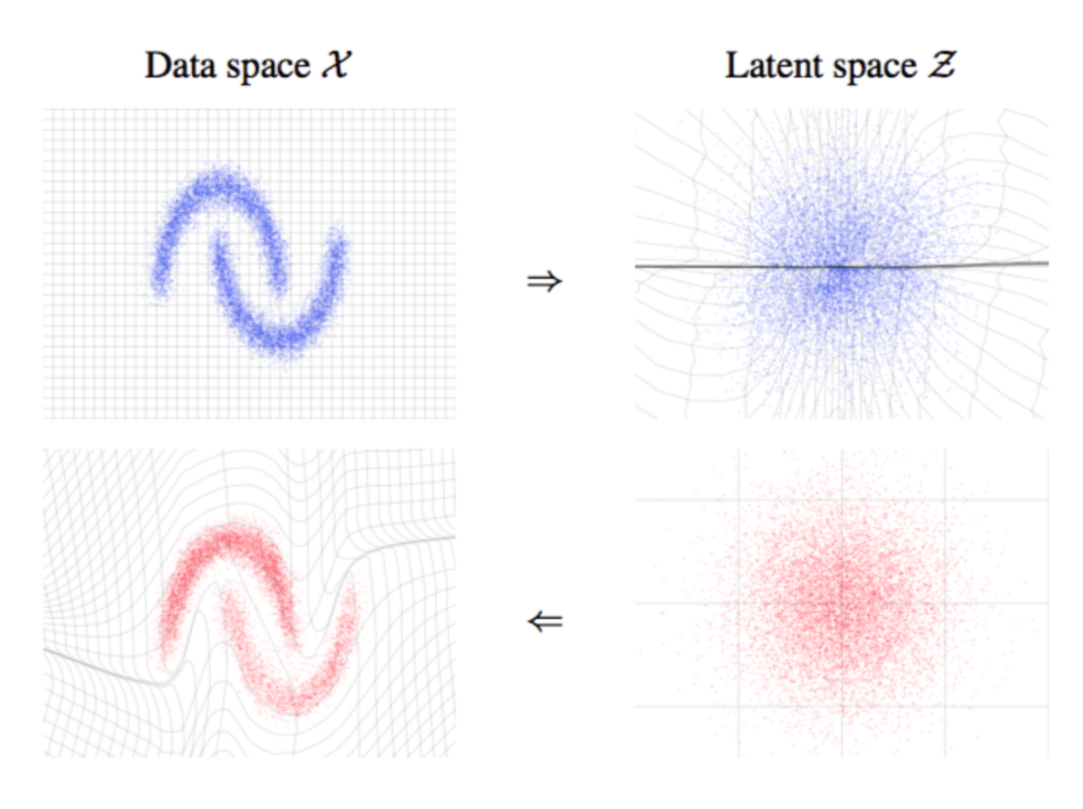
- 左图展示了归一化流(Normalizing Flow)的核心思想:通过一系列可逆变换在数据空间与潜在空间之间建立一一对应关系。
- 在左侧的数据空间 \(\mathcal{X} \) 中,原始数据分布是复杂的(例如弯曲的双 moons 形流形);通过学习到的可逆映射,将其逐步“拉直”并变换到右侧的潜在空间 \(\mathcal{Z} \),使其变为简单的标准分布(如各向同性高斯)。反过来,从简单的潜在分布采样,再通过逆变换映射回数据空间,就可以生成复杂结构的数据。
- 关键点是:整个变换过程是双射(bijective)且可计算雅可比行列式,从而可以精确地进行概率密度的变换与建模。
# AI for PE
Normalizing Flows
base density
target density
Train
nflow
# AI for PE
Normalizing Flows
base density
target density
Train
nflow
Test
nflow
nflow
nflow
# AI for PE
Normalizing Flows
base density
target density
Conditioner 的思路框架图 (略)
( . , a )
( . , b)
( . , a+b)
( . , hidden_dims)
Linear
BN+ReLU+Linear
+BN+ReLU
+Dropout+Linear
( . , hidden_dims)
num_layers x
( . , hidden_dims)
Flow input
Context
Linear
( . , 2 x hidden_dims)
( . , hidden_dims)
copy
( . , hidden_dims)
( . , hidden_dims)
( . , a)
Cat
Cat
GLU
Flow output
num_blocks x
# AI for PE
(Based on 1912.02762)
1024 sec
8 sec
ref_time
GPS time
6 sec
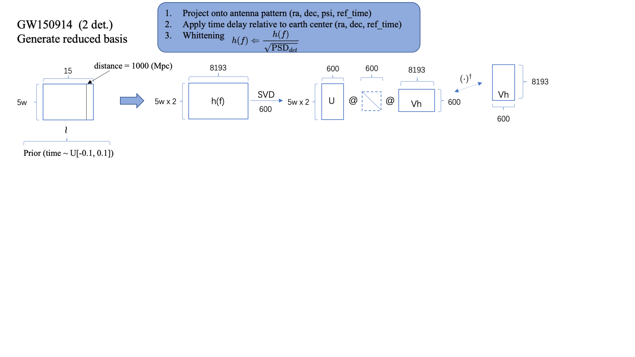
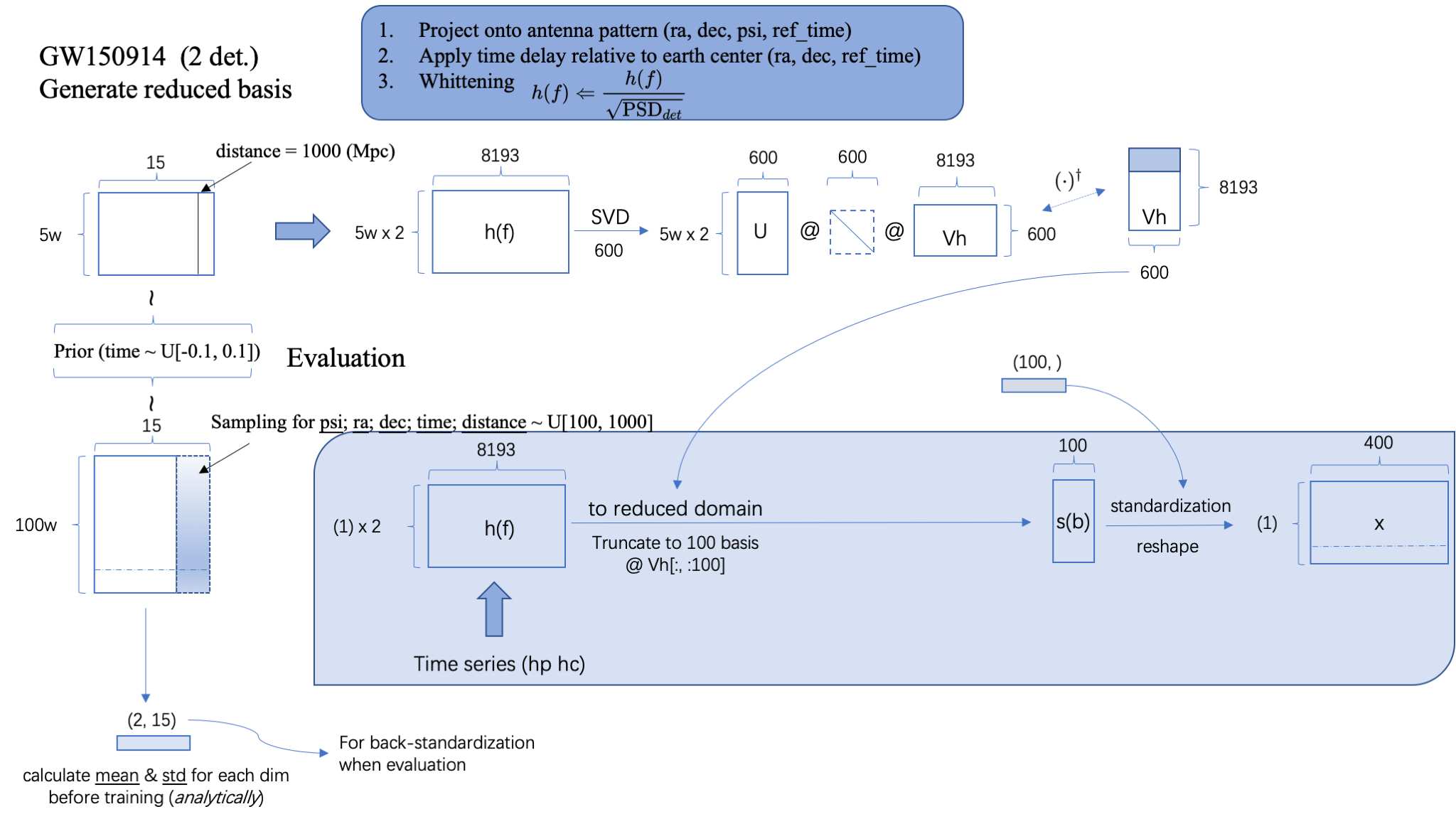
Step.1: Generate reduced basis based on SVD.
- 基于 Prior 在 15dim 参数空间上采样 5w 样本。
- 每个参数样本生成关于探测器的白化的频域引力波波形 \(h(f)\)(依赖于:探测器的 3 个方位参数+信号到达 GPS 时间+PSD)
- 取定 600 basis 进行 SVD 分解,本地保存基矢矩阵 Vh。
Step.1
Step.0
- Ref: Green S R, Gair J. Complete parameter inference for GW150914 using deep learning[J]. Machine Learning: Science and Technology, 2021, 2(3): 03LT01.
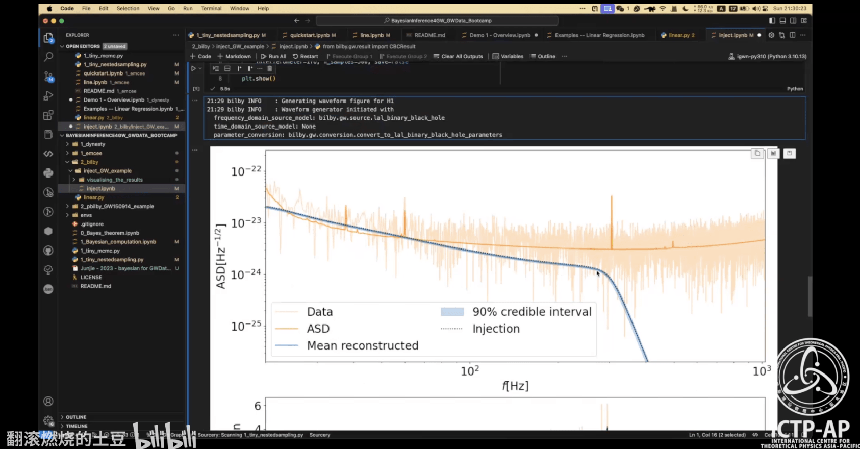
Step.0: Estimate PSD around the target event.
- 取 LIGO 记录的 8 sec 时域引力波数据,其中假定信号位于第 6 sec 附近 \(\pm0.1\) sec 内。
- 根据该事件信号附近 1024 sec 的时域引力波数据,估计噪声功率谱密度,即 PSD。
# AI for PE
Training
1024 sec
8 sec
ref_time
GPS time
6 sec
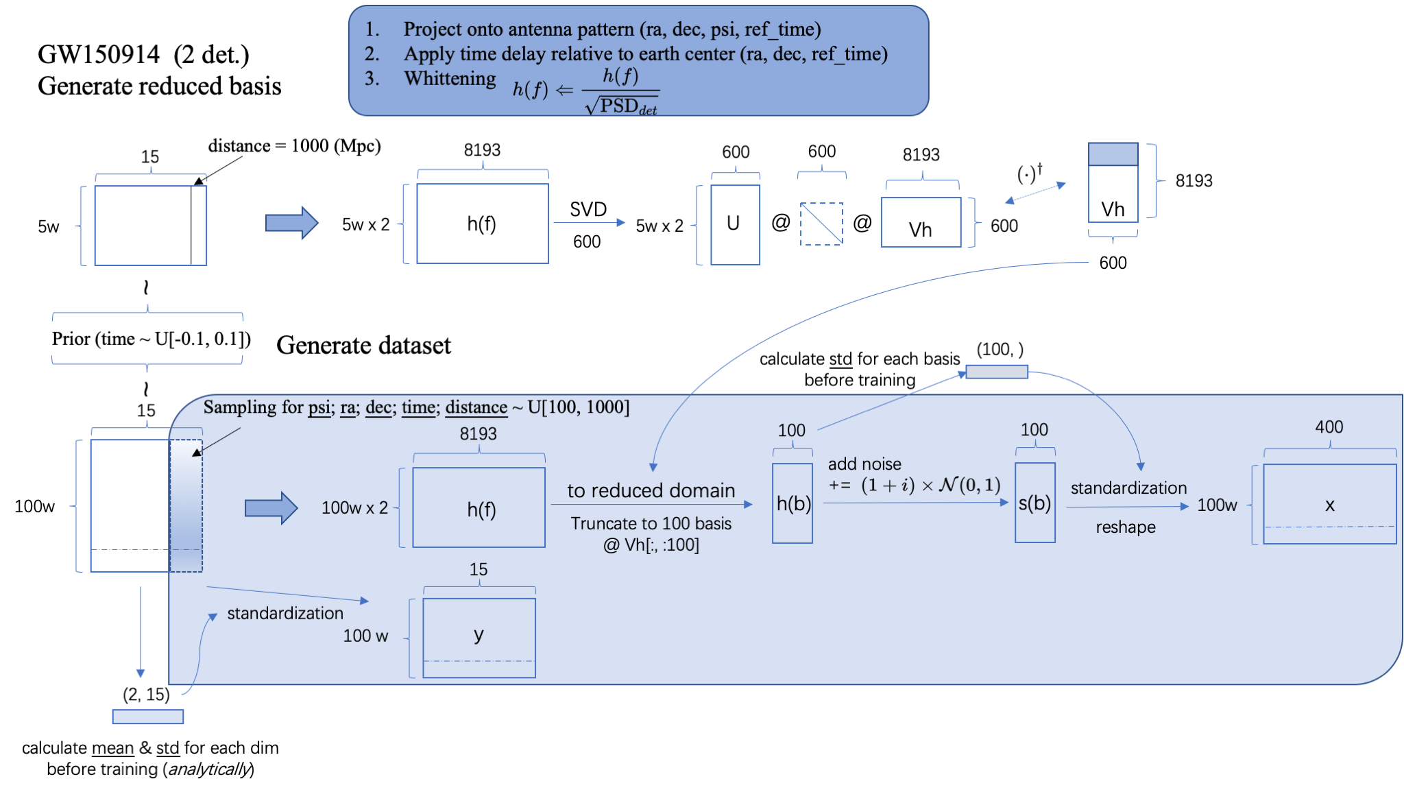
Step.2: Train the model
- 基于 Prior 在 15dim 参数空间上采样 100w 样本,并根据先验分布的每个维度解析地计算 mean 和 std 以备用于标准化 flow 的输入数据。
- 训练迭代过程:
- 重新采样探测器方位角参数、distance 和到达时间 time,根据每个样本生成关于探测器的白化的频域引力波波形 \(h(f)\)(依赖于:探测器的 3 个方位参数+信号到达 GPS 时间+PSD) 考虑 2 个独立探测器,因此波形共计 200w 个。经过标准化给出每个样本 15 维参数 \(y\) 作为 flow 的输入数据。
- 将频域波形映射到 reduced space 上。即读取本地的基矢矩阵 Vh,将频域波形 \(h(f)\) 的特征维度 8193 降到 600,再进一步截断取前 100 维作为波形 \(h(b)\) 的特征维度。
- 计算并保存 100 个 basis 维度的 std,以备用于标准化 flow 的 conditioner 数据。
- 在 \(h(b)\) 上进一步添加高斯白噪声 + 标准化 + reshape 为每个样本有 400 个特征维度(2 探测器 x 实部虚部 2 部分 x 原 100 特征维度 ),得到 flow 的 conditioner: \(x\)。
- 以 \(y\) 作为 target distribution 的输入数据,\(x\) 作为 conditioner,在 flow 模型中映射到 base distribution 上可得到 15 个特征维度 100w 个数据。计算其在高斯概率分布上的交叉熵损失,即 loss。
- Ref: Green S R, Gair J. Complete parameter inference for GW150914 using deep learning[J]. Machine Learning: Science and Technology, 2021, 2(3): 03LT01.
Step.2
base dist.
target dist.
Coupling architecture:
Rational Quadratic Neural Spline Flows (RQ-NSF)
# AI for PE
1024 sec
8 sec
ref_time
GPS time
6 sec
Testing
Step.3: Test the model (inference)
- 输入极化的时域引力波数据 \(h_p,h_c\),根据该样本生成关于探测器的白化的频域引力波波形 \(h(f)\)(依赖于:探测器的 3 个方位参数+信号到达 GPS 时间+PSD)
- 读取本地的基矢矩阵 Vh,将该频域波形映射到 reduced space 上,特征维度降到 100,再根据训练过程中保存的 100 个 basis 维度的 std 对数据进行标准化,得到 conditioner 数据 \(x\)。
- 在 flow 模型中,从 base distribution (高斯)上采样样本 \(N\) 个,以 \(x\) 数据作为条件,输出 target distribution 后验样本 \(N\) 个。
Step.3
base dist.
target dist.
- Ref: Green S R, Gair J. Complete parameter inference for GW150914 using deep learning[J]. Machine Learning: Science and Technology, 2021, 2(3): 03LT01.
# AI for PE
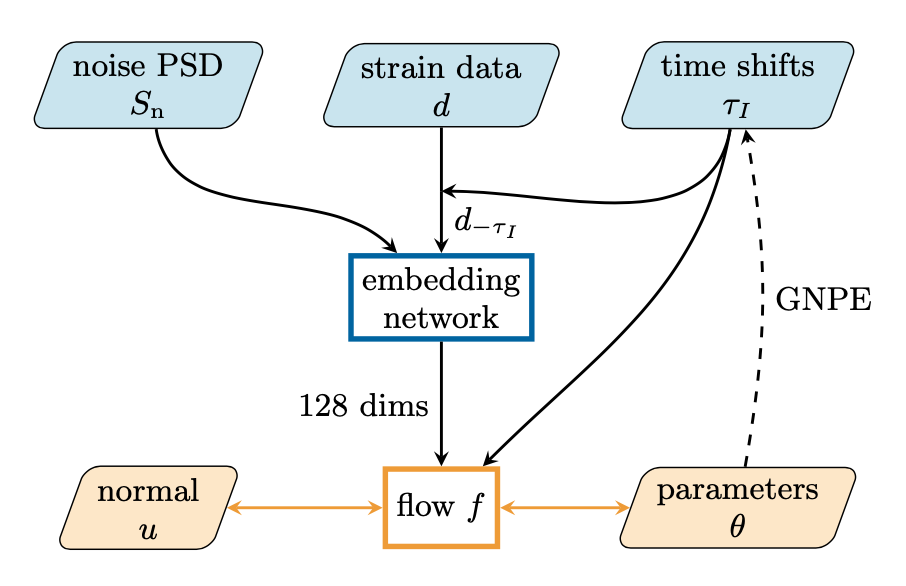
Training
1024 sec
8 sec
ref_time
GPS time
6 sec
200
200
200
800
128
Embedding network
num of residual block \(10 \rightarrow 5\)
num of flows \(15 \rightarrow 30\)
(1024, 512, 256, 128)
\(n\sim p(S_n)\)
\(S^{(i)}_n\sim p(S_n)\)
~28 days
~50 days
3 models
time shift
\(\delta t_I \sim \kappa(\delta t_I)\)
?
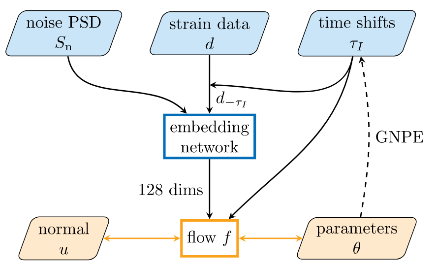
- Dax M, Green S R, Gair J, et al. Real-time gravitational-wave science with neural posterior estimation[J]. arXiv preprint arXiv:2106.12594, 2021
# AI for PE
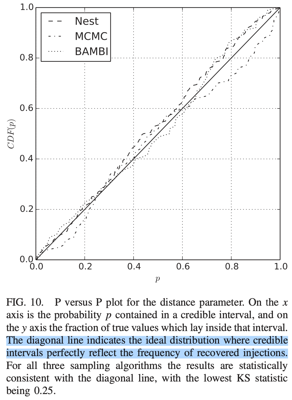
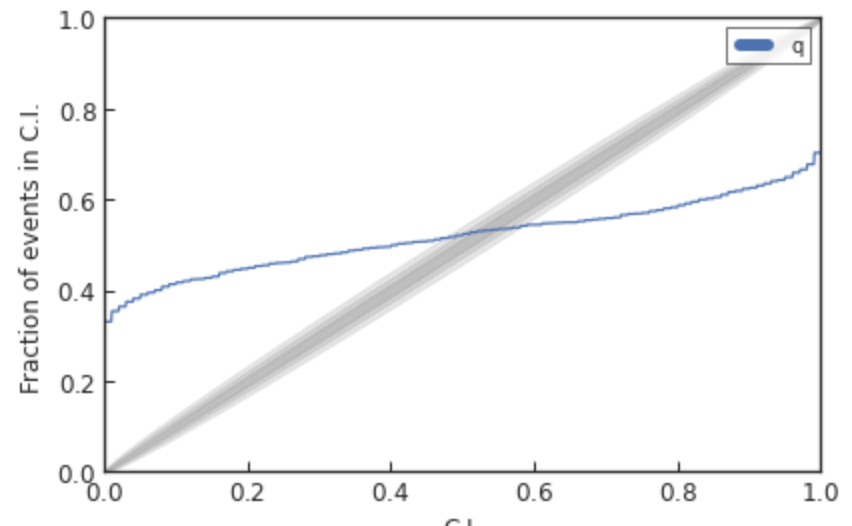
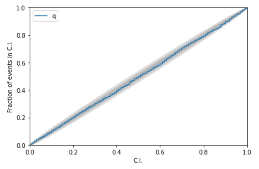
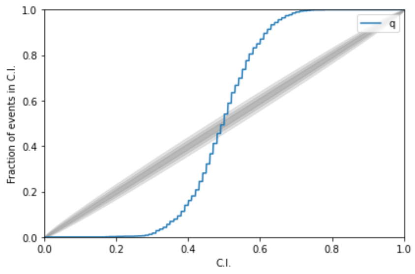
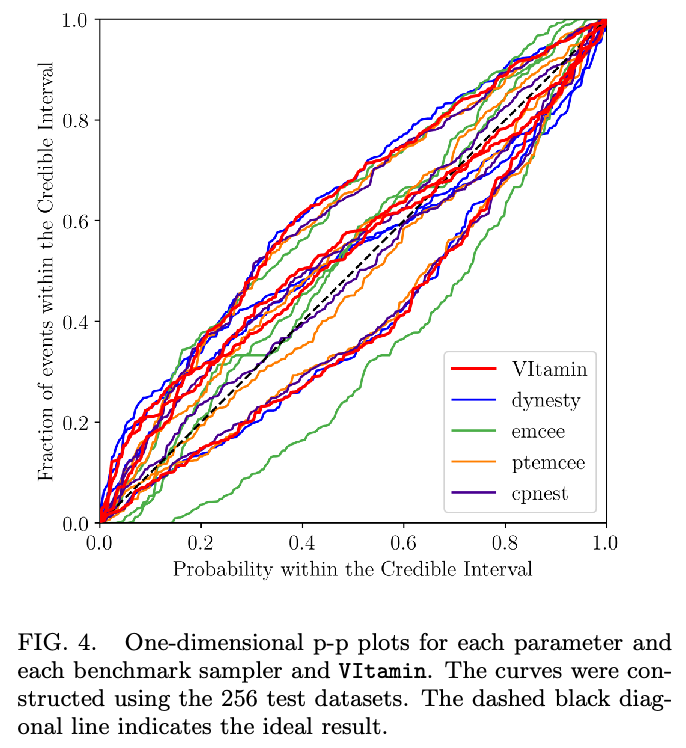
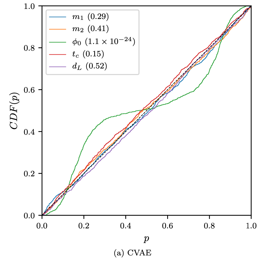
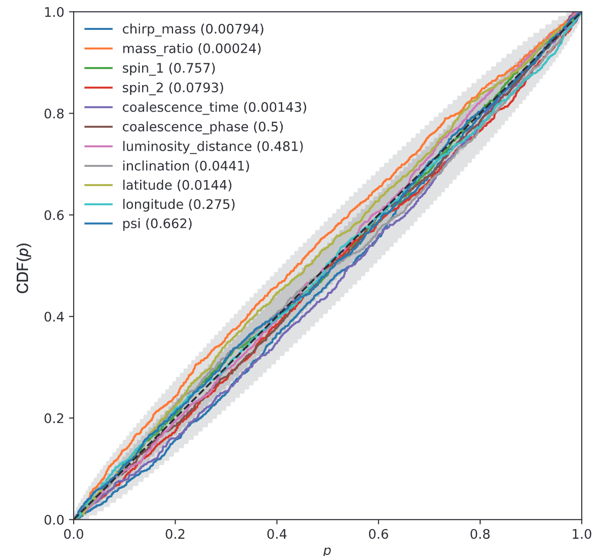
Kolmogorov-Smirnov (KS) Test & Confidence Intervals (C.I.)
A check to ensure that the probability distributions we recover are truly representative of the confidence we should hold in the parameters of the signal.
By setting up a large set of test injections we can see if this is statistically true by determining the frequency with which the true parameters lie within a certain confidence level.
For each run we calculate credible intervals from the posterior samples, for each parameter. We can then examine the number of times the injected value falls within a given credible interval. If the posterior samples are an unbiased estimate of the true probability, then 10% of the runs should find the injected values within a 10% credible interval, 50% of runs within the 50% interval, and so on.
(1409.7215)
Median-unbiased estimators involve random errors and no systematic errors.
def pp_plot_scratch(Posterior, TrueParams,
		x_values = np.linspace(0, 1, 1001)):
    '''
    Posterior - (Num of injections, Num of sampleing)
    TrueParams - (Num of injections, )
    '''
    credible_levels = np.array([sum(pd.Series(Posterior[i]) < T)/len(Posterior[i]) \
    				for i, T in enumerate(TrueParams)])
    pp = np.array([sum(credible_levels < xx) /
                       len(credible_levels) for xx in x_values])
    return pp
# AI for PE
Kolmogorov-Smirnov (KS) Test & Confidence Intervals (C.I.)
A check to ensure that the probability distributions we recover are truly representative of the confidence we should hold in the parameters of the signal.
(1409.7215)
A test for pp-plot:
# AI for PE
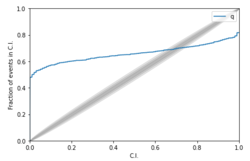
Kolmogorov-Smirnov (KS) Test & Confidence Intervals (C.I.)
A check to ensure that the probability distributions we recover are truly representative of the confidence we should hold in the parameters of the signal.
(1409.7215)
A test for pp-plot:
# AI for PE
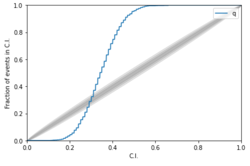
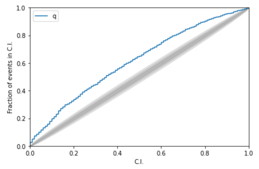
Kolmogorov-Smirnov (KS) Test & Confidence Intervals (C.I.)
A check to ensure that the probability distributions we recover are truly representative of the confidence we should hold in the parameters of the signal.
(1409.7215)

(2008.03312)
(2002.07656)
(1909.06296)
Some cases:
# AI for PE
Simulation-based Inference (SBI)
for GW parameter estimation
-
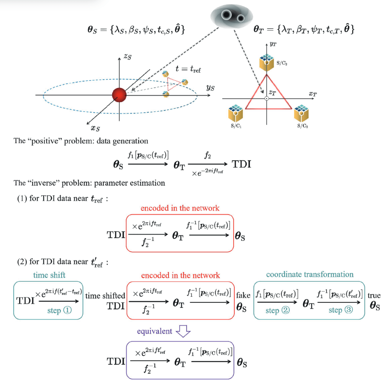
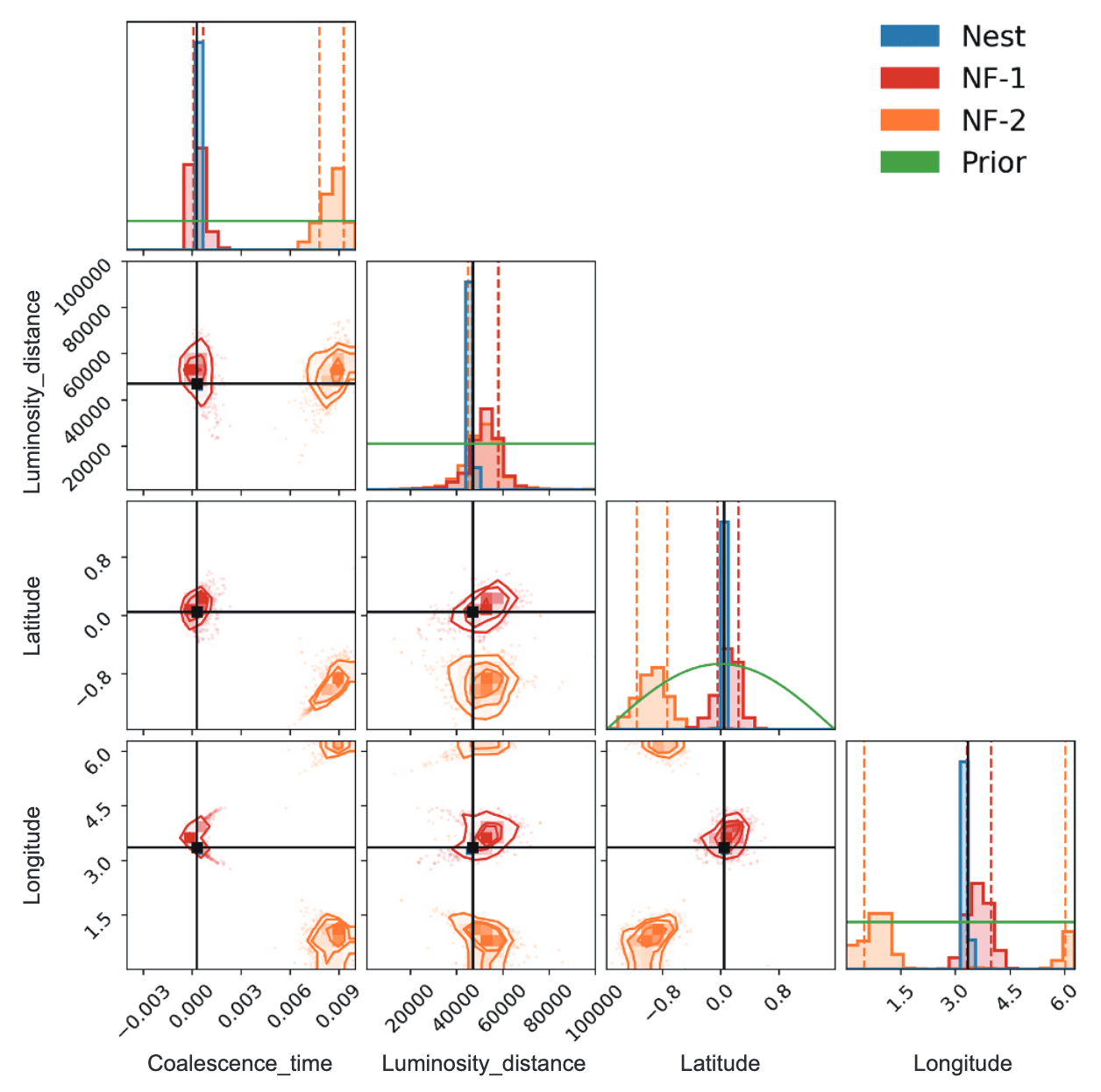
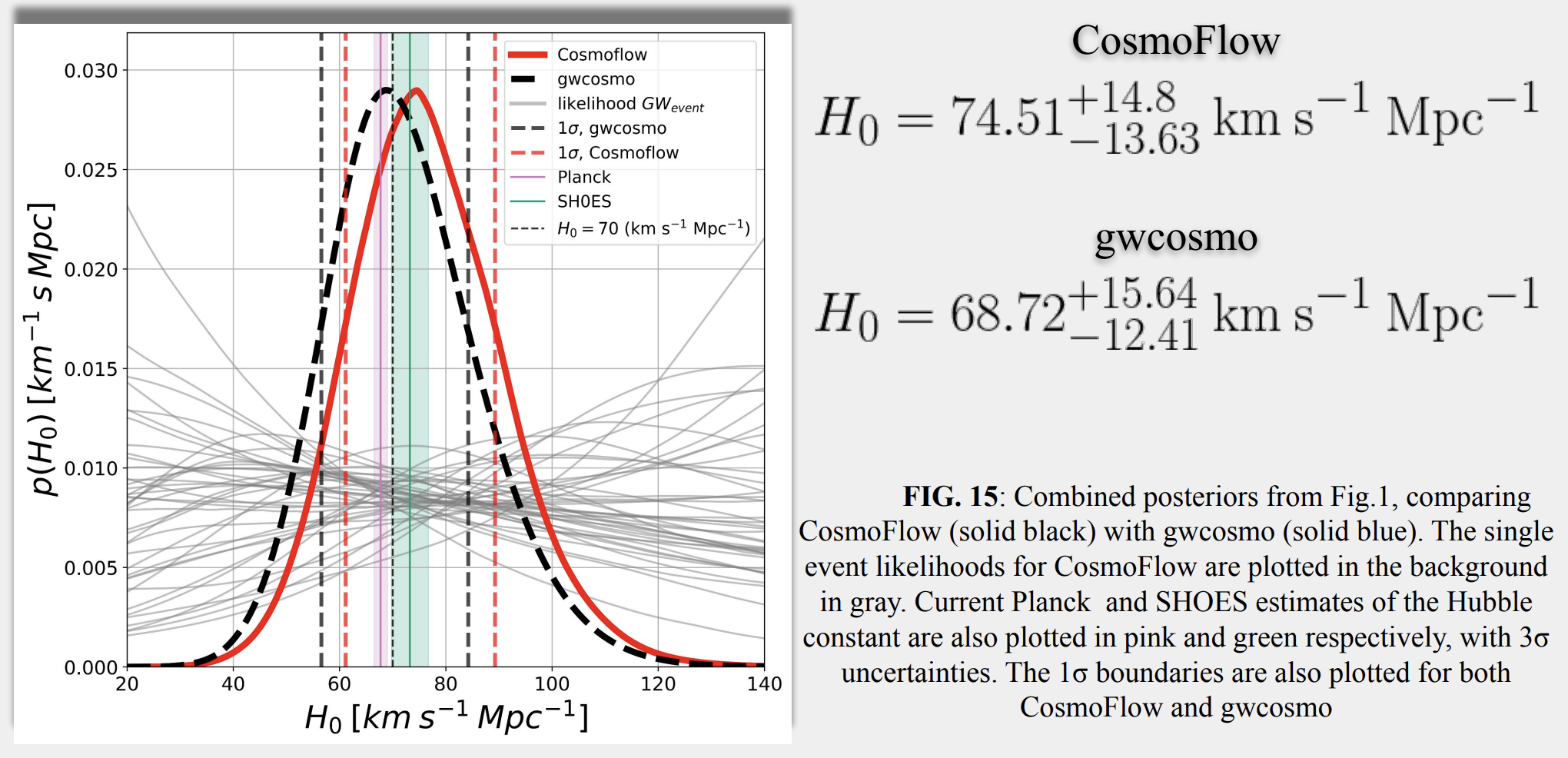
🚀 针对空间引力波探测中大规模黑洞双星(MBHB)在复杂噪声背景下的参数快速估计挑战,该研究提出了一种基于可伸缩Normalizing Flow (NF) 模型的方法。
-
💡 该方法创新性地简化了数据复杂度,并利用变换映射克服了Taiji一年周期时间依赖响应函数的挑战,实现了对11维MBHB参数的全面无偏估计。
-
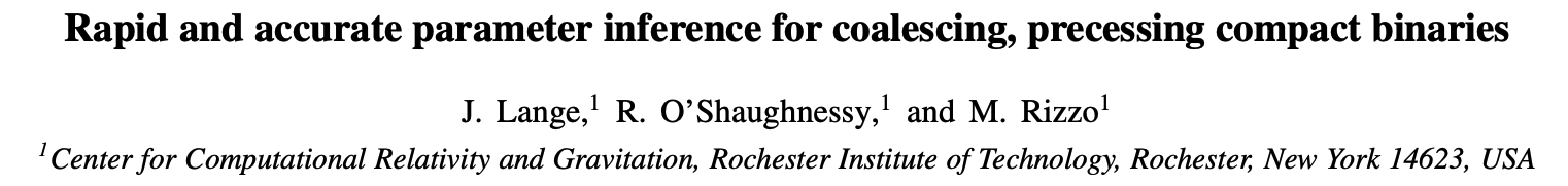
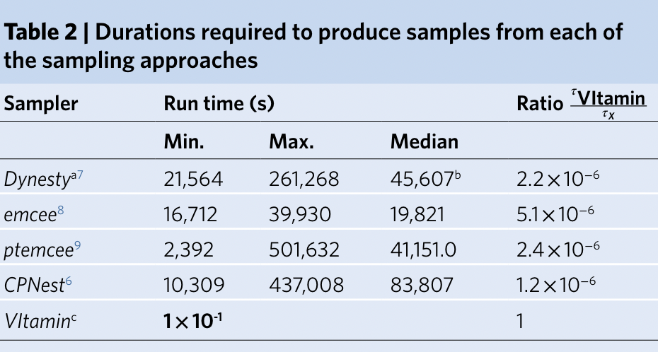
✨ 结果表明,该方法比传统技术快几个数量级,同时保持高精度,并揭示了到达时间参数中以前未见的额外多模态性,极大地提高了引力波数据分析效率。
# AI for PE
-
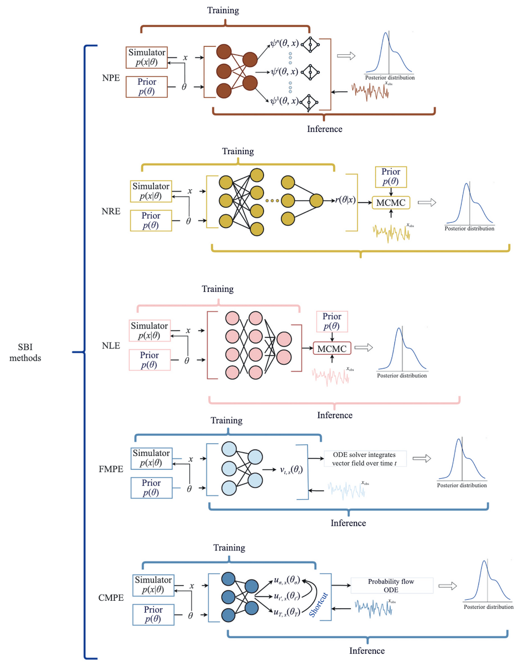
🌌 针对引力波数据分析中传统方法(如Markov chain Monte Carlo)面临的计算挑战,该综述探讨了基于机器学习的模拟推断(SBI)方法作为一种高效解决方案。
-
💫 论文详细阐述了Normalizing Flows、Neural Posterior Estimation (NPE)、Neural Ratio Estimation (NRE) 和 Flow Matching 等SBI技术,并展示了它们在单源参数估计、叠加信号分析、检验广义相对论及族群研究中的应用。
-
🚀 尽管SBI方法在速度上显著提升,但其模型依赖性、先验假设敏感性、可解释性及验证挑战仍是其广泛采纳的障碍,未来研究将着重于结合AI与传统方法的混合范式。
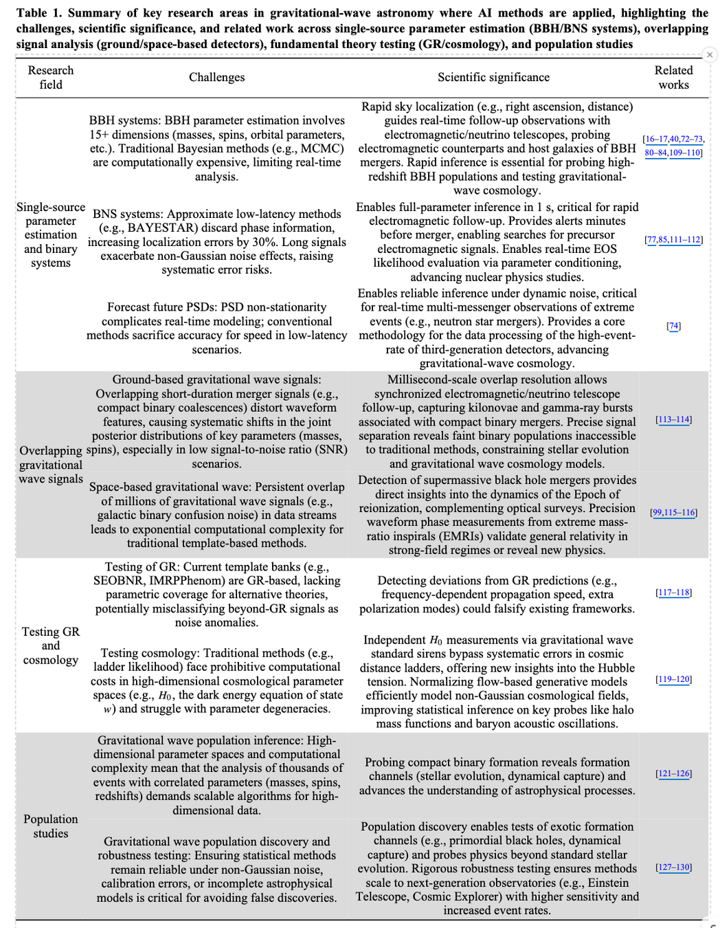
arXiv:2507.11192.
literature covered up to early 2025 only.
Simulation-based Inference (SBI)
for GW parameter estimation
# AI for PE
Key Takeaway
The "Real" Reasons We Apply ML to GW Astrophysics
Let's be honest about our motivations... 😉
The perfectly valid "scientific" reasons:
- ✓ It sounded like a cool project
- ✓ My supervisor said it was a good thing to work on
- ✓ I will learn some really useful ML skills
- ✓ I'm already good at ML
- ✓ I want to get better at ML
- ✓ I want to get a high-paying job after this PhD/postdoc
- ✓ I want to be spared when the machines take over
Credit: Chris Messenger (MLA meeting,, Jan 2025)
# AI for PE
Key Takeaway
Why is AI/ML Everywhere in GW Research?
The core motivations behind nearly all AI+GW research
ML is FAST
So much data, so little time!
• Bayesian parameter estimation
• Replaces computationally intensive components
ML is ACCURATE*
Consistently outperforms traditional approaches
• Unmodelled burst searches
• Continuous GW searches
ML is FLEXIBLE
Provides deeper insights into complex problems
• Reveals patterns through interpretability
• Enables previously impractical approaches
* When properly trained and validated on appropriate datasets
Credit: Chris Messenger (MLA meeting,, Jan 2025)
Credit: Chris Messenger (MLA meeting,, Jan 2025)
Key question: If an ML (or any) analysis doesn't do 1 or more of these things, then from a scientific perspective,
what is the point?
# AI for PE
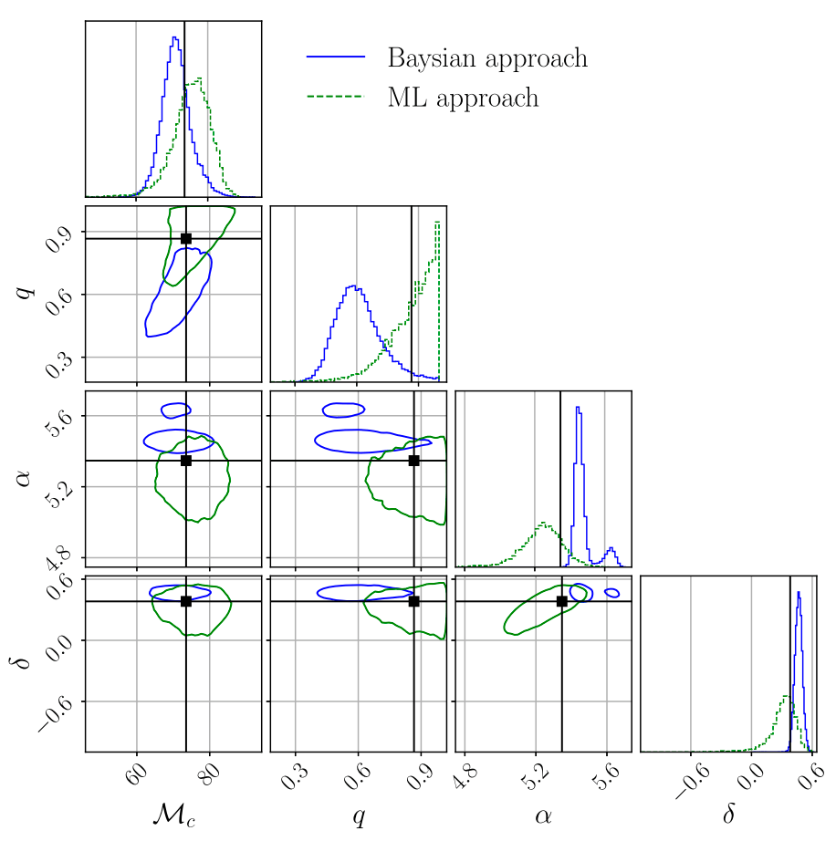
在用SBI等生成模型做参数估计(PE)时,社区里其实逐渐分化出两种不同的范式,可以概括为 Validation-driven 与 Discovery-driven:
- 第一种更“保守”的路径,是把流模型当作 MCMC 的加速器或替代实现。目标很明确:在相同似然、相同先验下,复现 MCMC 的后验结果(边缘分布、相关结构、多模态性等),只是速度更快、可扩展性更好。这一范式的说服力来自一致性——如果生成模型在系统误差可控的前提下与 MCMC 达到统计等价,那么它的价值主要体现在计算效率(例如实时或大规模事件处理)。在这个语境下,“没有新发现”反而是一种优点,因为它意味着方法学上是无偏替代。
- 另一种更“激进”的路径,则把生成模型视为一种可能揭示新结构的工具。这里的逻辑是:流模型(或更广义的神经后验估计)在表达能力、全局建模和高维耦合刻画上,可能捕捉到传统采样方法难以充分探索的后验特征(例如极窄模态、复杂退化方向,甚至由模型失配或噪声非高斯性引入的结构)。因此,如果生成模型系统性地给出与 MCMC 不同的结果,这不一定被视为错误,而可能被解读为潜在的新物理或新数据特征的信号。
Key Takeaway
arXiv:2310.13405, LIGO-P2300306
PRL 127, 24 (2021) 241103.
PRL 130, 17 (2023) 171403.
arXiv:2310.12209
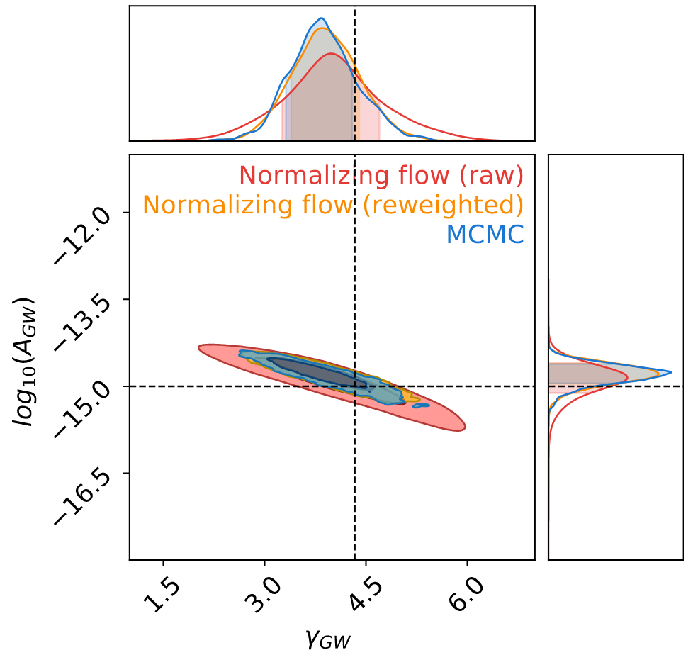
Fast Parameter Inference on Pulsar Timing Arrays with Normalizing Flows
arXiv:2404.14286
DOI:10.1103/PhysRevLett.130.171402
# AI for PE
Key Takeaway
Is It Really So Simple?
The reality of ML in scientific research is more nuanced
No: We need to think more critically
- ❓ Are we just trying to predict a function?
- ❓ Are there any astrophysical constraints?
- ❓ Do we need to understand how/why it works?
- ❓ What about errors? Quality flags?
- ❓ What happens if things go wrong?
Twitter: @DeepLearningAI_
# AI for PE
Key Takeaway
Why Even Use AI?
The mathematical inevitability and the path to understanding
Universal Approximation Theorem
The existence theorem that guarantees solutions
- Neural networks with sufficient hidden layers can approximate any continuous function on compact subsets of \(\mathbb{R}^n\)
- Ref: Cybenko, G. (1989), Hornik et al. (1989)
The solution is mathematically guaranteed — our challenge is finding the path to it
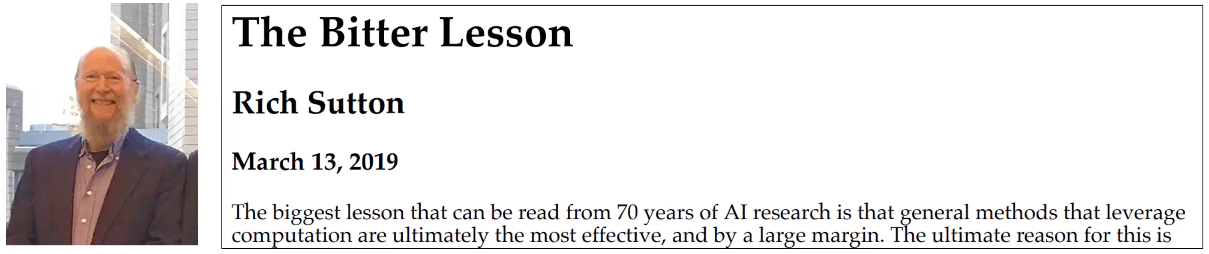
Machine learning will win in the long run
AI models still have vast potential compared to the human brain's efficiency. Beating traditional methods is mathematically inevitable given sufficient resources.
The question is not if AI/ML will win, but how
Understanding AI's inner workings is the real challenge, not proving its capabilities.
That's where we can learn something exciting with Foundation Models.
# AI for PE
一个不可回避的张力:
- 在 Validation 范式 下,“不同”通常首先被归因为模型误差、训练偏差或近似误差;
- 在 Discovery 范式 下,“不同”则被赋予物理意义,但前提是你能够排除前者。
因此,一个更现实的中间路径往往是:先在受控设置中完成对 MCMC 的严格对齐(包括覆盖率、校准性、极端尾部行为等),建立可信度;再在真实复杂数据(如非高斯噪声、模型不完备)中系统性地分析偏差来源。如果差异在多种独立实现、不同架构与数据切片下保持稳健,并且能被物理或仪器效应解释,那么才有资格被讨论为“发现”。
换句话说:要么作为无偏加速器被验证;要么对偏差来源给出可解释的物理或统计依据。
Key Takeaway
arXiv:2310.13405, LIGO-P2300306
PRL 127, 24 (2021) 241103.
PRL 130, 17 (2023) 171403.
arXiv:2310.12209
Fast Parameter Inference on Pulsar Timing Arrays with Normalizing Flows
arXiv:2404.14286
DOI:10.1103/PhysRevLett.130.171402
Fast is easy to claim. Better needs an explanation.
引力波数据探索:编程与分析实战训练营
结营仪式与课程总结
主讲老师:王赫
2024/01/14
ICTP-AP, UCAS
- 训练营课程回顾与总结
- 课程报名与参与人员情况
- 教学知识点罗列+自我提升的途径+全新的作业提交模型
- 作业完成情况 & 竞赛排名情况(提及高中生朋友,请吃饭)
- 颁奖典礼(竞赛前三名讲解题思路?代表发言?)
- 后记
- 感谢主办方和曙光的大力支持(主办方发言?曙光代表发言?)
- 课程团队的收获与感恩,对我来说也是一种技能提升
- 赶DDL完成作业没那么容易吧?嘿嘿嘿。。。
- 可以理解很多同学很忙,但也看到不少同学“很用心”
- 录屏分享 + B 站开通+记得给课程star(迁移到ICTP的gitlab上)
- 欢迎更多的反馈:关于太极计划、引力波物理、数理统计与数据分析、PyTorch系统性课程、高效科研工具分享、现代科研方法与学术写作套路、与同学和导师等人际关系、学术圈生存手册、卷的动力学原理初探、通向自我实现之路、如何发现适合自己的人生。。。
- 见到我,记得和我打招呼
。。。
致谢

- 主办单位
- 中国科学院大学 · 国际理论物理中心(亚太地区)
- 中国科学院大学 - 引力波宇宙太极实验室
- 赞助单位
- 中科曙光


| 但易 | 活动策划+算力支持 |
| ... |

| 田昕峣 | 特邀嘉宾 |
| 赵俊杰 | 特邀嘉宾 |
| 高民权 | 特邀嘉宾 |
训练营课程回顾与总结
# GWData: Bootcamp
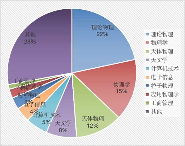
- 训练营报名初期,有效申请的学员人数共 432 人,来自各行各业。其中一半以上来自理论物理、物理学、天体物理和天文学等专业方向。
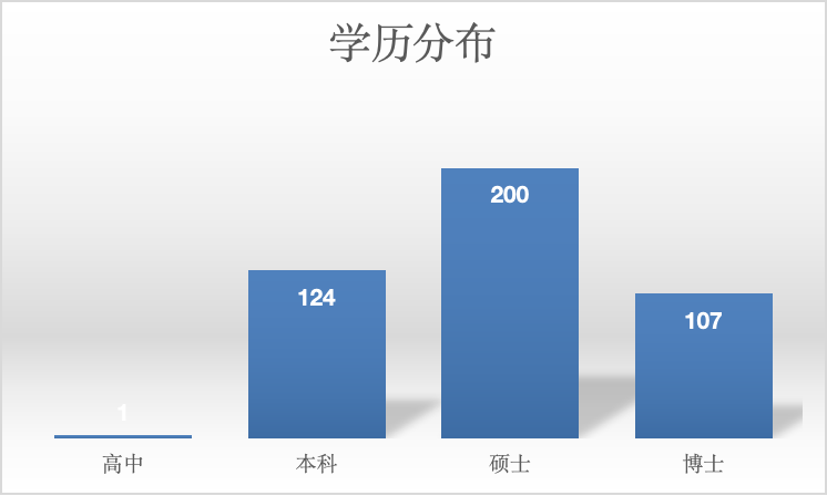
- 在“其他”专业类别中,包含心理学、生物信息与医药、工商管理、材料与化工、地震与地球物理、金融、控制工程等等。

- 在学员填写的 “个人研究的主要障碍” 和 “对本课程的期望” 的词云分析中,“引力波”、“机器学习”、“数据处理”、“深度学习”、“能力”、“编程”等是最常见的关键词。
- 课程报名与参与人员情况

训练营课程回顾与总结
# GWData: Bootcamp
- 教学大纲与实战项目
- 通向自我实现之路
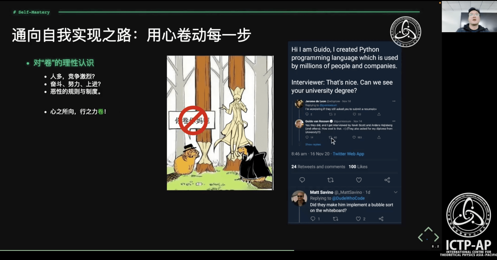
- 对“卷”的理性认识
- 做研究所需要的范式转换
- 做好笔记是自我学习的不二捷径
- 自学路上必会之 “上下求索"的技能
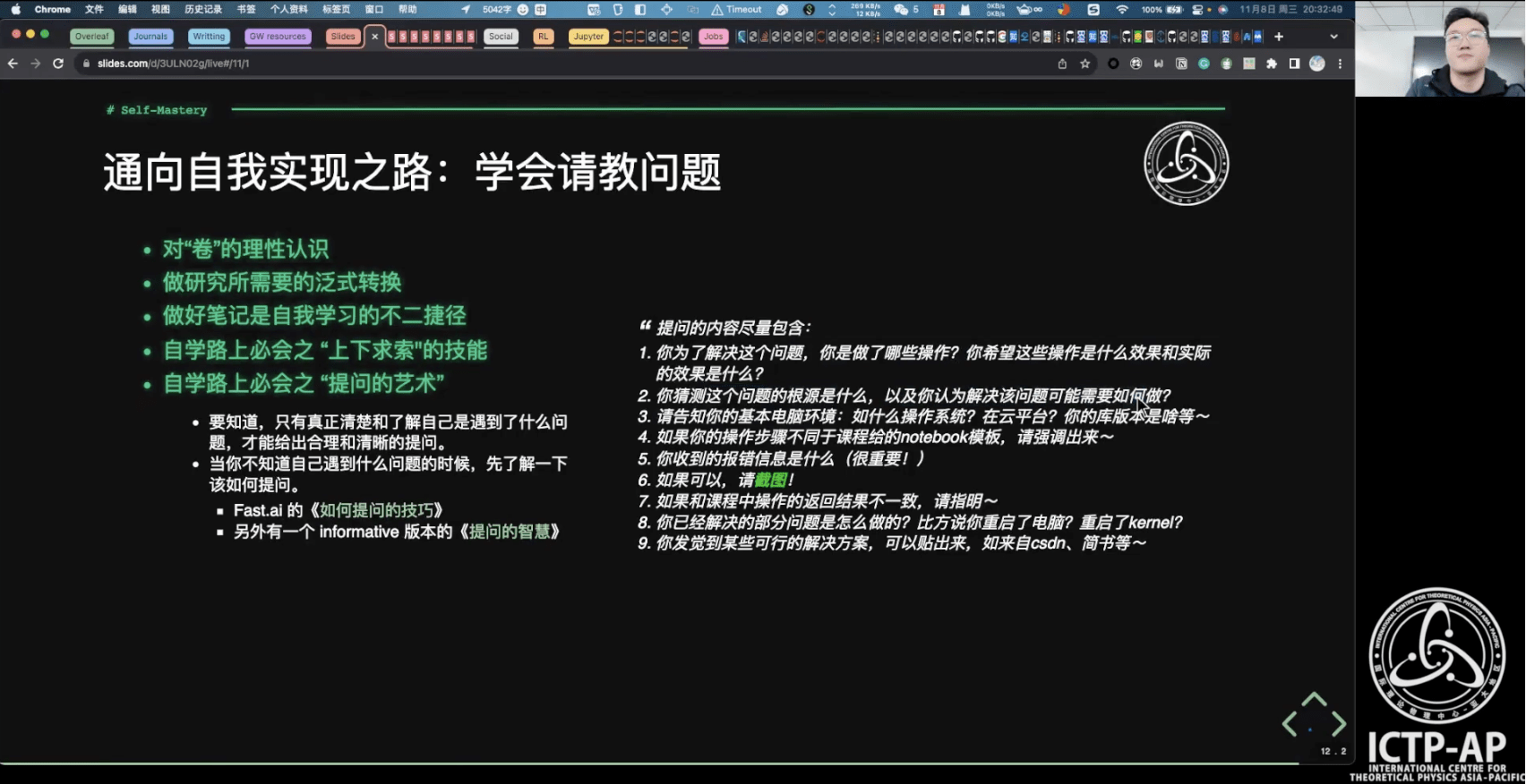
- 自学路上必会之 “提问的艺术”
- 第 0 部分:打鸡血!
- 通向自我实现之路
- 第 1 部分:编程开发环境与工作流
- 基础运维技术
- 容器化技术
- 实战项目:Python / Jupyter 开发环境搭建 + 远程连接 VS Code
- 实战项目:LALsuite / LISAcode 的源码编译 (optional)
- Git 分布式版本控制系统
- 【公开课】数据技术演进与现实应用 (特邀嘉宾:田昕峣)
- 第 2 部分:基于 Python 的数据分析基础
- 数据科学语言 Python 从入门到熟悉
- 数据分析实训之 Numpy / Pandas
- 实战项目:GW Event Catalog 的探索性数据分析
- 实战项目:股票数据分析案例 (optional)
- 基于 Python 的数据可视化理论与实践之 Matplotlib / Seaborn
- 实战项目:GWTC 论文中的 Figures
- 实战项目:针对 GW150914 信号处理与匹配滤波数据分析
- 【公开课】贝叶斯推断在引力波科学中的应用 (特邀嘉宾:赵俊杰)
- 第 3 部分:机器学习基础
- 机器学习算法之应用起步
- 机器学习算法之应用进阶
- 实战项目:基于 LIGO 的 Glitch 元数据完成多分类任务
- 实战项目:基于 LIGO 的 Glitch 时频图数据实现聚类分析
- 第 4 部分:深度学习基础
- 深度学习技术概述与神经网络基础
- 实战项目:训练一个3层神经网络(手撸版)
- 卷积神经网络与引力波信号探测
- 实战项目:使用 CNN 识别双黑洞系统引力波信号
- Kaggle数据科学竞赛 (黑客马拉松): Can you find the GW signals?
- 【公开课】AI发展全景与GPT前沿解析 (特邀嘉宾:高民权)
训练营课程回顾与总结
# GWData: Bootcamp
- 教学大纲与实战项目
- 基础运维技术
- 什么是Linux/Shell;新手必须掌握的Linux命令
- 管道符、重定向与环境变量;SSH服务管理远端设备
- 容器化技术
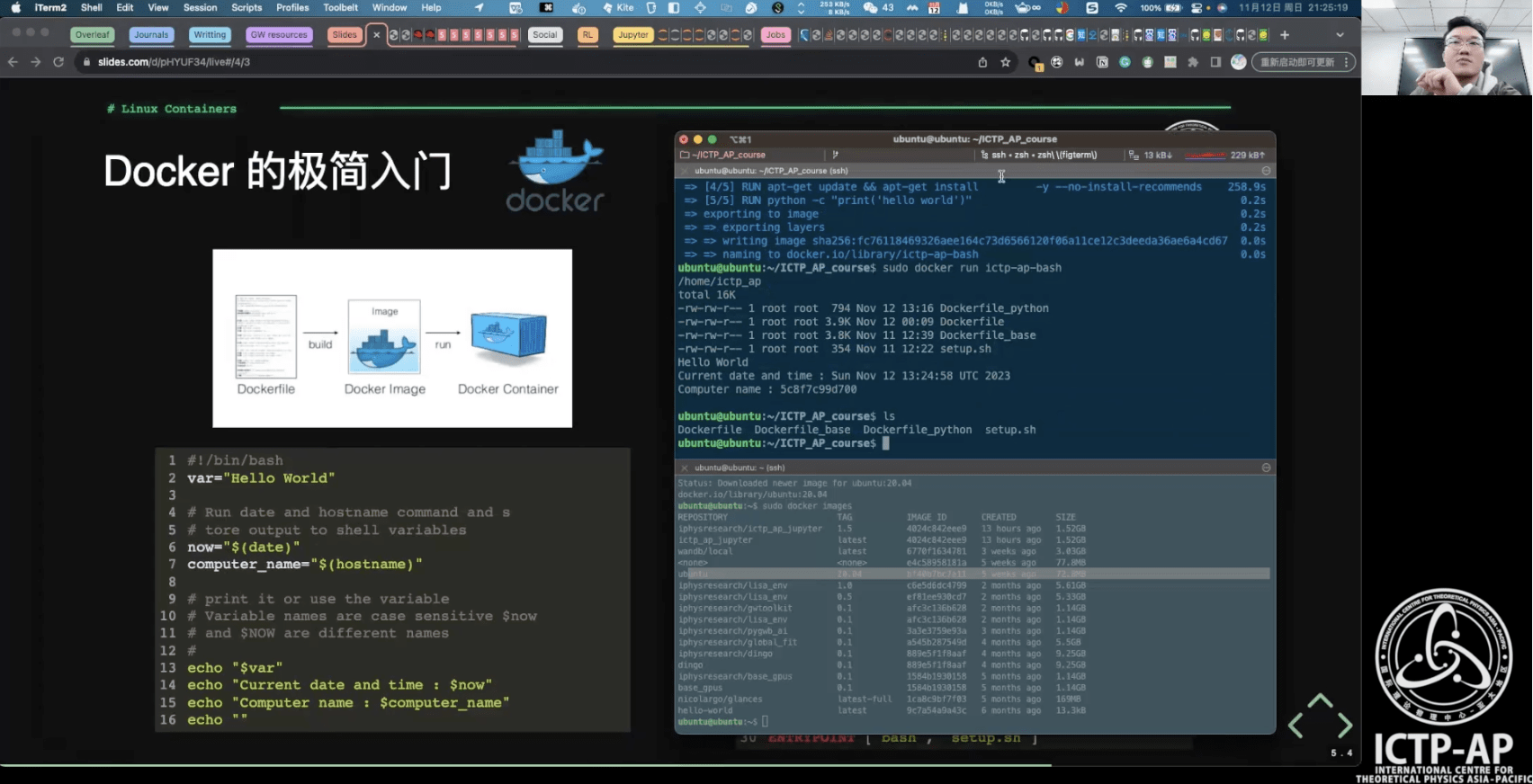
- Linux 容器虚拟化;Docker 的极简入门
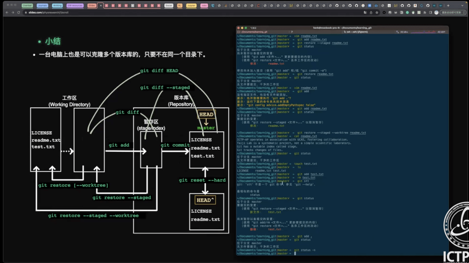
- Git 分布式版本控制系统
- Git 安装/创建版本库;工作区、暂存区、版本库
- 远程仓库;分支管理;Git 可视化管理工具


- 第 0 部分:打鸡血!
- 通向自我实现之路
- 第 1 部分:编程开发环境与工作流
- 基础运维技术
- 容器化技术
- 实战项目:Python / Jupyter 开发环境搭建 + 远程连接 VS Code
- 实战项目:LALsuite / LISAcode 的源码编译 (optional)
- Git 分布式版本控制系统
- 【公开课】数据技术演进与现实应用 (特邀嘉宾:田昕峣)
- 第 2 部分:基于 Python 的数据分析基础
- 数据科学语言 Python 从入门到熟悉
- 数据分析实训之 Numpy / Pandas
- 实战项目:GW Event Catalog 的探索性数据分析
- 实战项目:股票数据分析案例 (optional)
- 基于 Python 的数据可视化理论与实践之 Matplotlib / Seaborn
- 实战项目:GWTC 论文中的 Figures
- 实战项目:针对 GW150914 信号处理与匹配滤波数据分析
- 【公开课】贝叶斯推断在引力波科学中的应用 (特邀嘉宾:赵俊杰)
- 第 3 部分:机器学习基础
- 机器学习算法之应用起步
- 机器学习算法之应用进阶
- 实战项目:基于 LIGO 的 Glitch 元数据完成多分类任务
- 实战项目:基于 LIGO 的 Glitch 时频图数据实现聚类分析
- 第 4 部分:深度学习基础
- 深度学习技术概述与神经网络基础
- 实战项目:训练一个3层神经网络(手撸版)
- 卷积神经网络与引力波信号探测
- 实战项目:使用 CNN 识别双黑洞系统引力波信号
- Kaggle数据科学竞赛 (黑客马拉松): Can you find the GW signals?
- 【公开课】AI发展全景与GPT前沿解析 (特邀嘉宾:高民权)
训练营课程回顾与总结
# GWData: Bootcamp
- 教学大纲与实战项目
- 数据的起源
- 何谓数据?
- 现代数据技术的发展脉络
- 当前主流数据技术
- 关系型数据库 (RDBMS)
- 非关系型数据库 (Not-only SQL (NoSQL) Database)
- 大数据 (Big Data)
- 数据仓库 (Data Warehouse)
- 流式计算 (Stream Processing)
- 数据湖 (Data Lake)
- 数据湖仓 (Data Lakehouse)
- 思考:从数据的角度认识世界
- 推荐阅读
- 第 0 部分:打鸡血!
- 通向自我实现之路
- 第 1 部分:编程开发环境与工作流
- 基础运维技术
- 容器化技术
- 实战项目:Python / Jupyter 开发环境搭建 + 远程连接 VS Code
- 实战项目:LALsuite / LISAcode 的源码编译 (optional)
- Git 分布式版本控制系统
- 【公开课】数据技术演进与现实应用 (特邀嘉宾:田昕峣)
- 第 2 部分:基于 Python 的数据分析基础
- 数据科学语言 Python 从入门到熟悉
- 数据分析实训之 Numpy / Pandas
- 实战项目:GW Event Catalog 的探索性数据分析
- 实战项目:股票数据分析案例 (optional)
- 基于 Python 的数据可视化理论与实践之 Matplotlib / Seaborn
- 实战项目:GWTC 论文中的 Figures
- 实战项目:针对 GW150914 信号处理与匹配滤波数据分析
- 【公开课】贝叶斯推断在引力波科学中的应用 (特邀嘉宾:赵俊杰)
- 第 3 部分:机器学习基础
- 机器学习算法之应用起步
- 机器学习算法之应用进阶
- 实战项目:基于 LIGO 的 Glitch 元数据完成多分类任务
- 实战项目:基于 LIGO 的 Glitch 时频图数据实现聚类分析
- 第 4 部分:深度学习基础
- 深度学习技术概述与神经网络基础
- 实战项目:训练一个3层神经网络(手撸版)
- 卷积神经网络与引力波信号探测
- 实战项目:使用 CNN 识别双黑洞系统引力波信号
- Kaggle数据科学竞赛 (黑客马拉松): Can you find the GW signals?
- 【公开课】AI发展全景与GPT前沿解析 (特邀嘉宾:高民权)
训练营课程回顾与总结
# GWData: Bootcamp
- 教学大纲与实战项目
- LIGO Open Data
- FFT by Scratch
- Spectral Analysis by Scratch
- Data analysis on GW150914
- Matched filtering to find the signal


- 第 0 部分:打鸡血!
- 通向自我实现之路
- 第 1 部分:编程开发环境与工作流
- 基础运维技术
- 容器化技术
- 实战项目:Python / Jupyter 开发环境搭建 + 远程连接 VS Code
- 实战项目:LALsuite / LISAcode 的源码编译 (optional)
- Git 分布式版本控制系统
- 【公开课】数据技术演进与现实应用 (特邀嘉宾:田昕峣)
- 第 2 部分:基于 Python 的数据分析基础
- 数据科学语言 Python 从入门到熟悉
- 数据分析实训之 Numpy / Pandas
- 实战项目:GW Event Catalog 的探索性数据分析
- 实战项目:股票数据分析案例 (optional)
- 基于 Python 的数据可视化理论与实践之 Matplotlib / Seaborn
- 实战项目:GWTC 论文中的 Figures
- 实战项目:针对 GW150914 信号处理与匹配滤波数据分析
- 【公开课】贝叶斯推断在引力波科学中的应用 (特邀嘉宾:赵俊杰)
- 第 3 部分:机器学习基础
- 机器学习算法之应用起步
- 机器学习算法之应用进阶
- 实战项目:基于 LIGO 的 Glitch 元数据完成多分类任务
- 实战项目:基于 LIGO 的 Glitch 时频图数据实现聚类分析
- 第 4 部分:深度学习基础
- 深度学习技术概述与神经网络基础
- 实战项目:训练一个3层神经网络(手撸版)
- 卷积神经网络与引力波信号探测
- 实战项目:使用 CNN 识别双黑洞系统引力波信号
- Kaggle数据科学竞赛 (黑客马拉松): Can you find the GW signals?
- 【公开课】AI发展全景与GPT前沿解析 (特邀嘉宾:高民权)
训练营课程回顾与总结
# GWData: Bootcamp
- 教学大纲与实战项目
- Brief introduction to gravitational wave (引力波简要介绍)
- Part I: Bayesian inference (贝叶斯推断)
- Part II: Bayesian computation (贝叶斯计算方法)
- Markov Chain Monte Carlo (MCMC; 马尔可夫链-蒙特卡罗方法)
- Nested sampling (嵌套采样)
- Part III: All in gravitational-wave data (一切尽在引力波数据中)
- Use Bilby & Parallel Bilby in the GW data analysis
- Show the complete pipeline for the data analysis
- The AMAZING Thomas Bayes (为美好的世界献上"贝叶斯定理")
- 第 0 部分:打鸡血!
- 通向自我实现之路
- 第 1 部分:编程开发环境与工作流
- 基础运维技术
- 容器化技术
- 实战项目:Python / Jupyter 开发环境搭建 + 远程连接 VS Code
- 实战项目:LALsuite / LISAcode 的源码编译 (optional)
- Git 分布式版本控制系统
- 【公开课】数据技术演进与现实应用 (特邀嘉宾:田昕峣)
- 第 2 部分:基于 Python 的数据分析基础
- 数据科学语言 Python 从入门到熟悉
- 数据分析实训之 Numpy / Pandas
- 实战项目:GW Event Catalog 的探索性数据分析
- 实战项目:股票数据分析案例 (optional)
- 基于 Python 的数据可视化理论与实践之 Matplotlib / Seaborn
- 实战项目:GWTC 论文中的 Figures
- 实战项目:针对 GW150914 信号处理与匹配滤波数据分析
- 【公开课】贝叶斯推断在引力波科学中的应用 (特邀嘉宾:赵俊杰)
- 第 3 部分:机器学习基础
- 机器学习算法之应用起步
- 机器学习算法之应用进阶
- 实战项目:基于 LIGO 的 Glitch 元数据完成多分类任务
- 实战项目:基于 LIGO 的 Glitch 时频图数据实现聚类分析
- 第 4 部分:深度学习基础
- 深度学习技术概述与神经网络基础
- 实战项目:训练一个3层神经网络(手撸版)
- 卷积神经网络与引力波信号探测
- 实战项目:使用 CNN 识别双黑洞系统引力波信号
- Kaggle数据科学竞赛 (黑客马拉松): Can you find the GW signals?
- 【公开课】AI发展全景与GPT前沿解析 (特邀嘉宾:高民权)
训练营课程回顾与总结
# GWData: Bootcamp
- 教学大纲与实战项目
- 人工智能 > 机器学习 > 深度学习
- 机器学习的定义,目标和过程
- 机器学习的常见类型
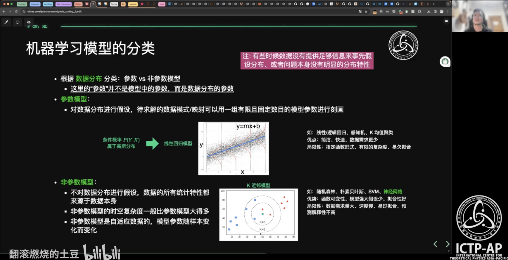
- 机器学习模型的分类
- 机器学习项目开发规划与准备及其开发步骤
- scikit-learn 机器学习库:分类+回归
- 机器学习中的模型调优与模型融合
- 特征工程
- 交叉验证
- 网格搜索
- 集成学习

- 第 0 部分:打鸡血!
- 通向自我实现之路
- 第 1 部分:编程开发环境与工作流
- 基础运维技术
- 容器化技术
- 实战项目:Python / Jupyter 开发环境搭建 + 远程连接 VS Code
- 实战项目:LALsuite / LISAcode 的源码编译 (optional)
- Git 分布式版本控制系统
- 【公开课】数据技术演进与现实应用 (特邀嘉宾:田昕峣)
- 第 2 部分:基于 Python 的数据分析基础
- 数据科学语言 Python 从入门到熟悉
- 数据分析实训之 Numpy / Pandas
- 实战项目:GW Event Catalog 的探索性数据分析
- 实战项目:股票数据分析案例 (optional)
- 基于 Python 的数据可视化理论与实践之 Matplotlib / Seaborn
- 实战项目:GWTC 论文中的 Figures
- 实战项目:针对 GW150914 信号处理与匹配滤波数据分析
- 【公开课】贝叶斯推断在引力波科学中的应用 (特邀嘉宾:赵俊杰)
- 第 3 部分:机器学习基础
- 机器学习算法之应用起步
- 机器学习算法之应用进阶
- 实战项目:基于 LIGO 的 Glitch 元数据完成多分类任务
- 实战项目:基于 LIGO 的 Glitch 时频图数据实现聚类分析
- 第 4 部分:深度学习基础
- 深度学习技术概述与神经网络基础
- 实战项目:训练一个3层神经网络(手撸版)
- 卷积神经网络与引力波信号探测
- 实战项目:使用 CNN 识别双黑洞系统引力波信号
- Kaggle数据科学竞赛 (黑客马拉松): Can you find the GW signals?
- 【公开课】AI发展全景与GPT前沿解析 (特邀嘉宾:高民权)
训练营课程回顾与总结
# GWData: Bootcamp
- 教学大纲与实战项目
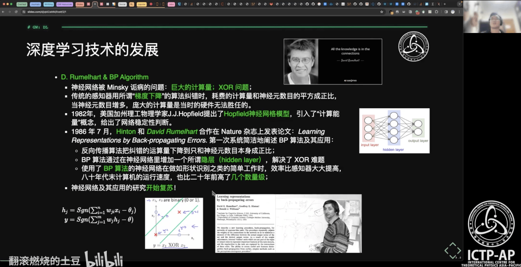
- 深度学习技术的起源、应用、特点
- 人工智能技术自学材料推荐
- 深度学习技术的“不能”
- 深度学习:神经网络基础
- 模型性能评估与测试调优
- 一维、二维卷积
- 引力波信号搜寻:卷积神经网络


- 第 0 部分:打鸡血!
- 通向自我实现之路
- 第 1 部分:编程开发环境与工作流
- 基础运维技术
- 容器化技术
- 实战项目:Python / Jupyter 开发环境搭建 + 远程连接 VS Code
- 实战项目:LALsuite / LISAcode 的源码编译 (optional)
- Git 分布式版本控制系统
- 【公开课】数据技术演进与现实应用 (特邀嘉宾:田昕峣)
- 第 2 部分:基于 Python 的数据分析基础
- 数据科学语言 Python 从入门到熟悉
- 数据分析实训之 Numpy / Pandas
- 实战项目:GW Event Catalog 的探索性数据分析
- 实战项目:股票数据分析案例 (optional)
- 基于 Python 的数据可视化理论与实践之 Matplotlib / Seaborn
- 实战项目:GWTC 论文中的 Figures
- 实战项目:针对 GW150914 信号处理与匹配滤波数据分析
- 【公开课】贝叶斯推断在引力波科学中的应用 (特邀嘉宾:赵俊杰)
- 第 3 部分:机器学习基础
- 机器学习算法之应用起步
- 机器学习算法之应用进阶
- 实战项目:基于 LIGO 的 Glitch 元数据完成多分类任务
- 实战项目:基于 LIGO 的 Glitch 时频图数据实现聚类分析
- 第 4 部分:深度学习基础
- 深度学习技术概述与神经网络基础
- 实战项目:训练一个3层神经网络(手撸版)
- 卷积神经网络与引力波信号探测
- 实战项目:使用 CNN 识别双黑洞系统引力波信号
- Kaggle数据科学竞赛 (黑客马拉松): Can you find the GW signals?
- 【公开课】AI发展全景与GPT前沿解析 (特邀嘉宾:高民权)
训练营课程回顾与总结
# GWData: Bootcamp
- 教学大纲与实战项目
-
Why AI Was Proposed
-
Earliest Form of AI and Solutions
-
Similarities between AI and Physics Methodologies
-
From Symbolic Systems to Machine Learning
-
Principles of Deep Learning
-
Breakthroughs Brought by Deep Learning
-
Typical Deep Learning Scenarios
-
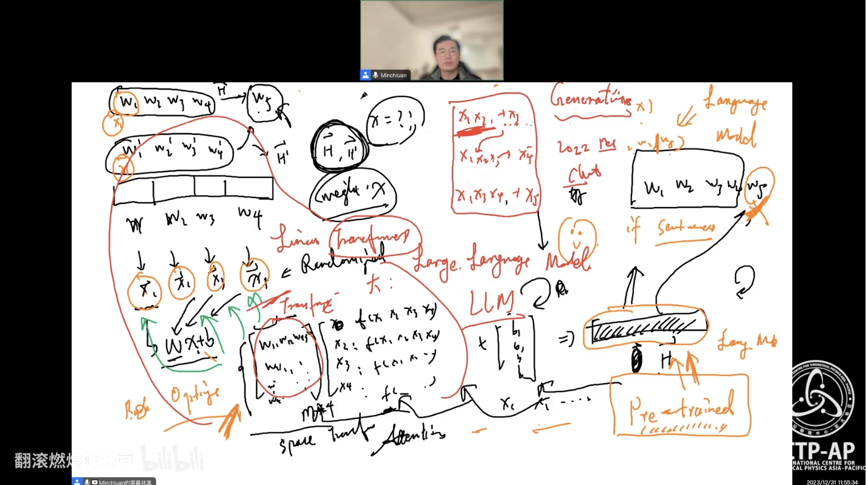
Pre-trained Models and Large Models
-
Principles of GPT
-
Breakthroughs in AIGC (AI Generated Content)
-
Current Challenges in AI
-
Frontiers of AI Research
- 第 0 部分:打鸡血!
- 通向自我实现之路
- 第 1 部分:编程开发环境与工作流
- 基础运维技术
- 容器化技术
- 实战项目:Python / Jupyter 开发环境搭建 + 远程连接 VS Code
- 实战项目:LALsuite / LISAcode 的源码编译 (optional)
- Git 分布式版本控制系统
- 【公开课】数据技术演进与现实应用 (特邀嘉宾:田昕峣)
- 第 2 部分:基于 Python 的数据分析基础
- 数据科学语言 Python 从入门到熟悉
- 数据分析实训之 Numpy / Pandas
- 实战项目:GW Event Catalog 的探索性数据分析
- 实战项目:股票数据分析案例 (optional)
- 基于 Python 的数据可视化理论与实践之 Matplotlib / Seaborn
- 实战项目:GWTC 论文中的 Figures
- 实战项目:针对 GW150914 信号处理与匹配滤波数据分析
- 【公开课】贝叶斯推断在引力波科学中的应用 (特邀嘉宾:赵俊杰)
- 第 3 部分:机器学习基础
- 机器学习算法之应用起步
- 机器学习算法之应用进阶
- 实战项目:基于 LIGO 的 Glitch 元数据完成多分类任务
- 实战项目:基于 LIGO 的 Glitch 时频图数据实现聚类分析
- 第 4 部分:深度学习基础
- 深度学习技术概述与神经网络基础
- 实战项目:训练一个3层神经网络(手撸版)
- 卷积神经网络与引力波信号探测
- 实战项目:使用 CNN 识别双黑洞系统引力波信号
- Kaggle数据科学竞赛 (黑客马拉松): Can you find the GW signals?
- 【公开课】AI发展全景与GPT前沿解析 (特邀嘉宾:高民权)
训练营课程回顾与总结
# GWData: Bootcamp
- 如何登峰造极?(自我提升的途径)


- 第 0 部分:打鸡血!
- 通向自我实现之路
- 第 1 部分:编程开发环境与工作流
- 基础运维技术
- 容器化技术
- 实战项目:Python / Jupyter 开发环境搭建 + 远程连接 VS Code
- 实战项目:LALsuite / LISAcode 的源码编译 (optional)
- Git 分布式版本控制系统
- 【公开课】数据技术演进与现实应用 (特邀嘉宾:田昕峣)
- 第 2 部分:基于 Python 的数据分析基础
- 数据科学语言 Python 从入门到熟悉
- 数据分析实训之 Numpy / Pandas
- 实战项目:GW Event Catalog 的探索性数据分析
- 实战项目:股票数据分析案例 (optional)
- 基于 Python 的数据可视化理论与实践之 Matplotlib / Seaborn
- 实战项目:GWTC 论文中的 Figures
- 实战项目:针对 GW150914 信号处理与匹配滤波数据分析
- 【公开课】贝叶斯推断在引力波科学中的应用 (特邀嘉宾:赵俊杰)
- 第 3 部分:机器学习基础
- 机器学习算法之应用起步
- 机器学习算法之应用进阶
- 实战项目:基于 LIGO 的 Glitch 元数据完成多分类任务
- 实战项目:基于 LIGO 的 Glitch 时频图数据实现聚类分析
- 第 4 部分:深度学习基础
- 深度学习技术概述与神经网络基础
- 实战项目:训练一个3层神经网络(手撸版)
- 卷积神经网络与引力波信号探测
- 实战项目:使用 CNN 识别双黑洞系统引力波信号
- Kaggle数据科学竞赛 (黑客马拉松): Can you find the GW signals?
- 【公开课】AI发展全景与GPT前沿解析 (特邀嘉宾:高民权)
训练营课程回顾与总结
# GWData: Bootcamp
- 作业完成情况
- 第 0 部分:打鸡血!
- 通向自我实现之路
- 第 1 部分:编程开发环境与工作流
- 基础运维技术
- 容器化技术
- 实战项目:Python / Jupyter 开发环境搭建 + 远程连接 VS Code
- 实战项目:LALsuite / LISAcode 的源码编译 (optional)
- Git 分布式版本控制系统
- 【公开课】数据技术演进与现实应用 (特邀嘉宾:田昕峣)
- 第 2 部分:基于 Python 的数据分析基础
- 数据科学语言 Python 从入门到熟悉
- 数据分析实训之 Numpy / Pandas
- 实战项目:GW Event Catalog 的探索性数据分析
- 实战项目:股票数据分析案例 (optional)
- 基于 Python 的数据可视化理论与实践之 Matplotlib / Seaborn
- 实战项目:GWTC 论文中的 Figures
- 实战项目:针对 GW150914 信号处理与匹配滤波数据分析
- 【公开课】贝叶斯推断在引力波科学中的应用 (特邀嘉宾:赵俊杰)
- 第 3 部分:机器学习基础
- 机器学习算法之应用起步
- 机器学习算法之应用进阶
- 实战项目:基于 LIGO 的 Glitch 元数据完成多分类任务
- 实战项目:基于 LIGO 的 Glitch 时频图数据实现聚类分析
- 第 4 部分:深度学习基础
- 深度学习技术概述与神经网络基础
- 实战项目:训练一个3层神经网络(手撸版)
- 卷积神经网络与引力波信号探测
- 实战项目:使用 CNN 识别双黑洞系统引力波信号
- Kaggle数据科学竞赛 (黑客马拉松): Can you find the GW signals?
- 【公开课】AI发展全景与GPT前沿解析 (特邀嘉宾:高民权)
-
Python: 108 quizzes
-
Numpy: 10 quizzes
-
Pandas: 12 quizzes
-
LeetCode: 5 problems
-
Matplotlib: 4 datasets
-
Seaborn: 4 datasets
-
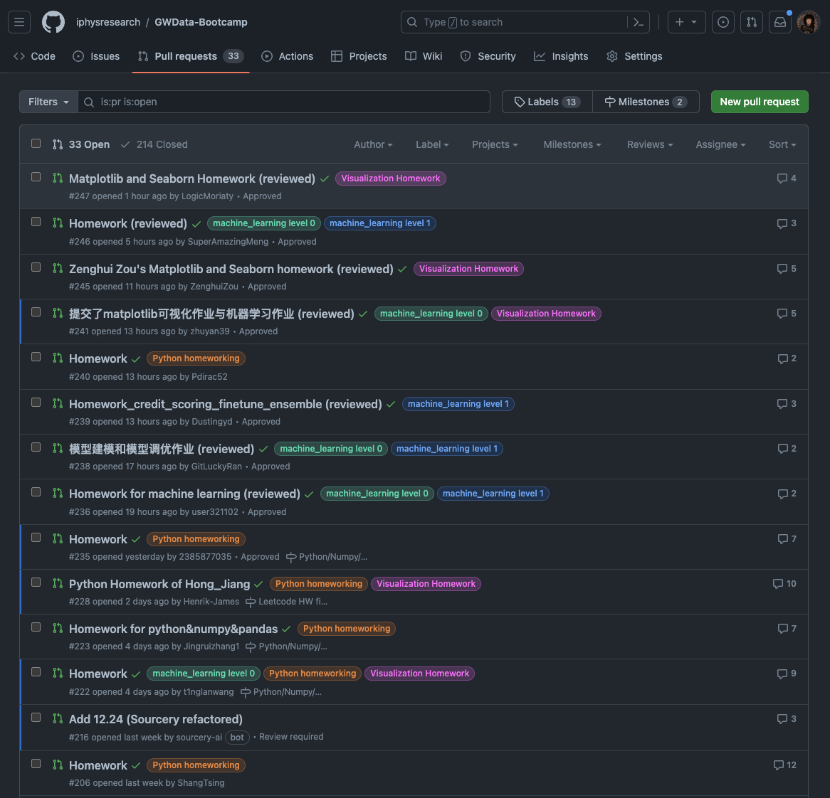
Git / GitHub: Pull Request
-
Credit Scoring dataset
-
Modeling
-
Finetune
-
-
Kaggle competition
-
Can you find the GW signal?
-
训练营课程回顾与总结
# GWData: Bootcamp
- 作业完成情况
| 总得分 | 1 | 2 | 3 | 4 | 5 | 6 | 7 |
|---|---|---|---|---|---|---|---|
| 频数 | 4 | 5 | 6 | 10 | 7 | 23 | 8 |
| 前#百分比排名 | 100.00% | 93.65% | 85.71% | 76.19% | 60.32% | 49.21% | 12.70% |
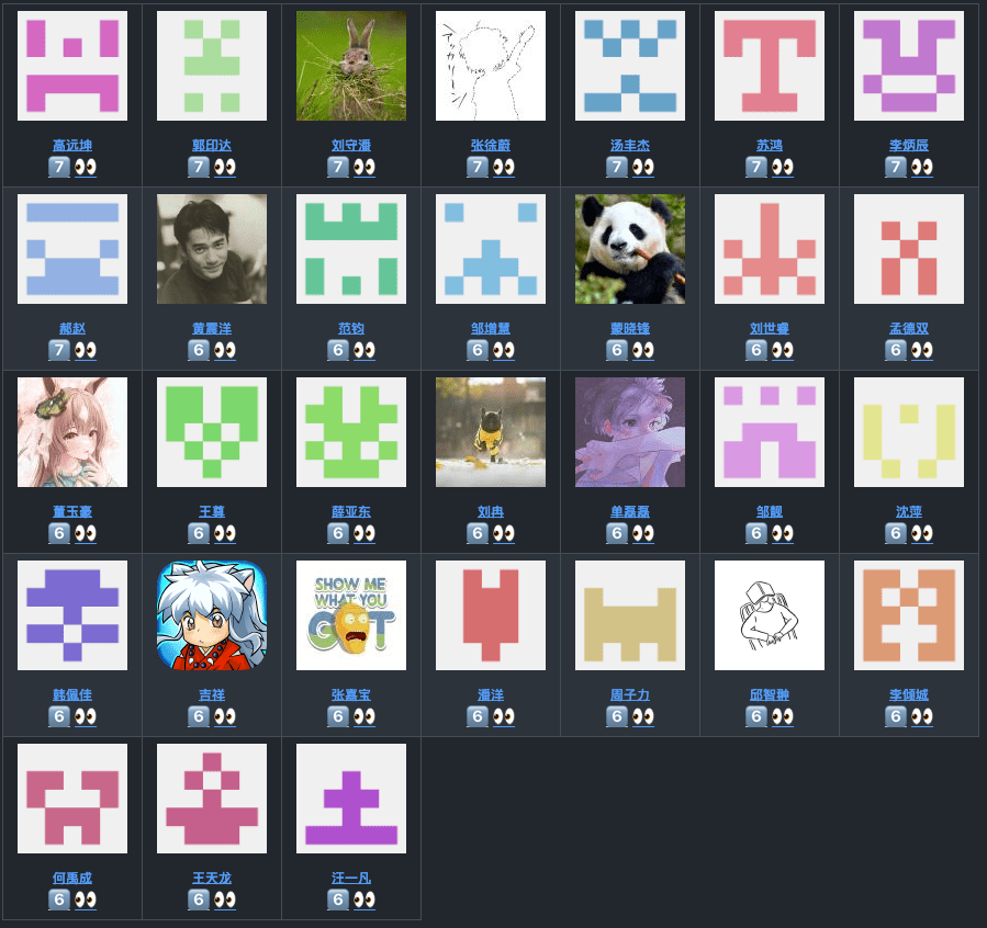
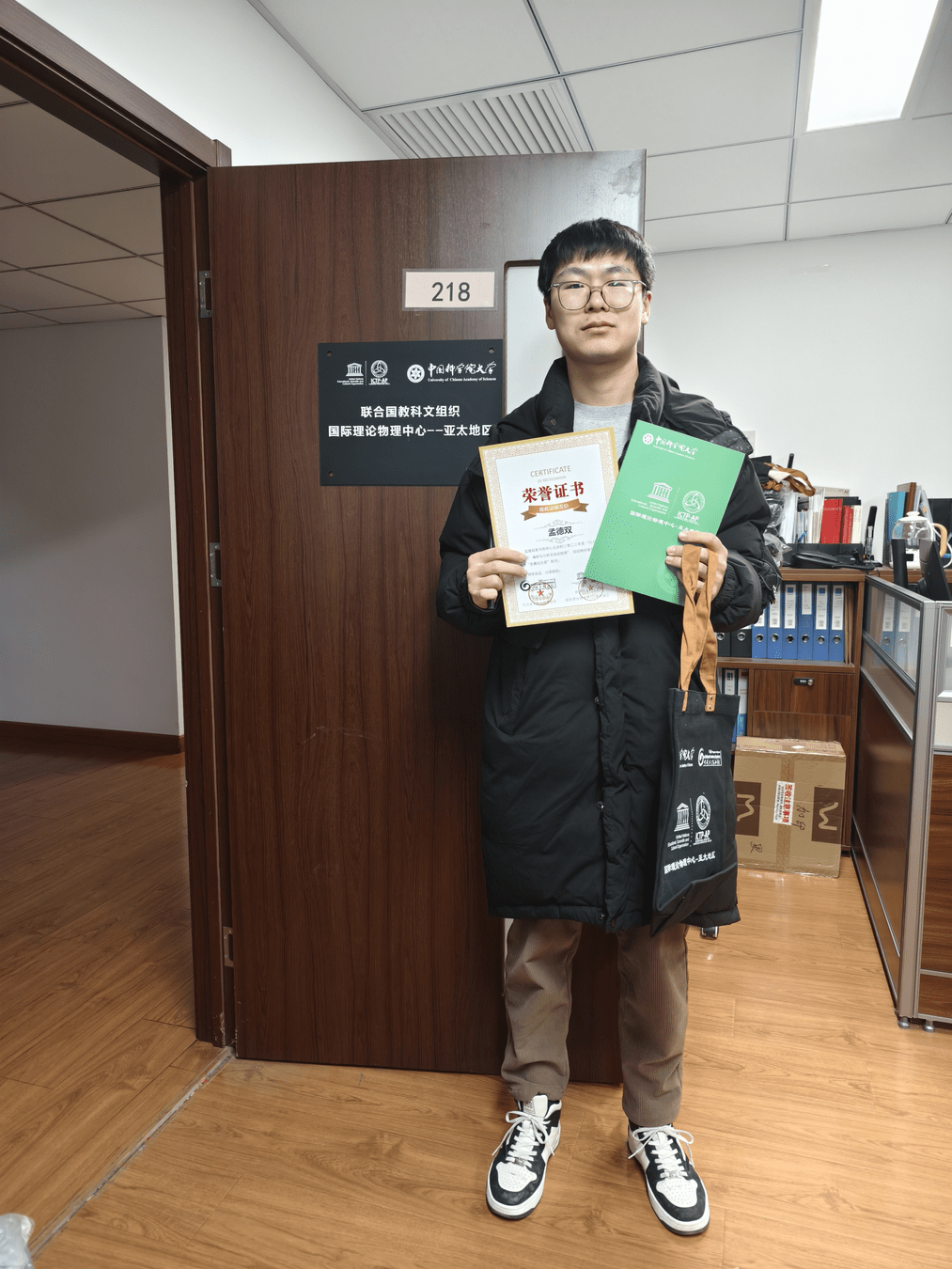
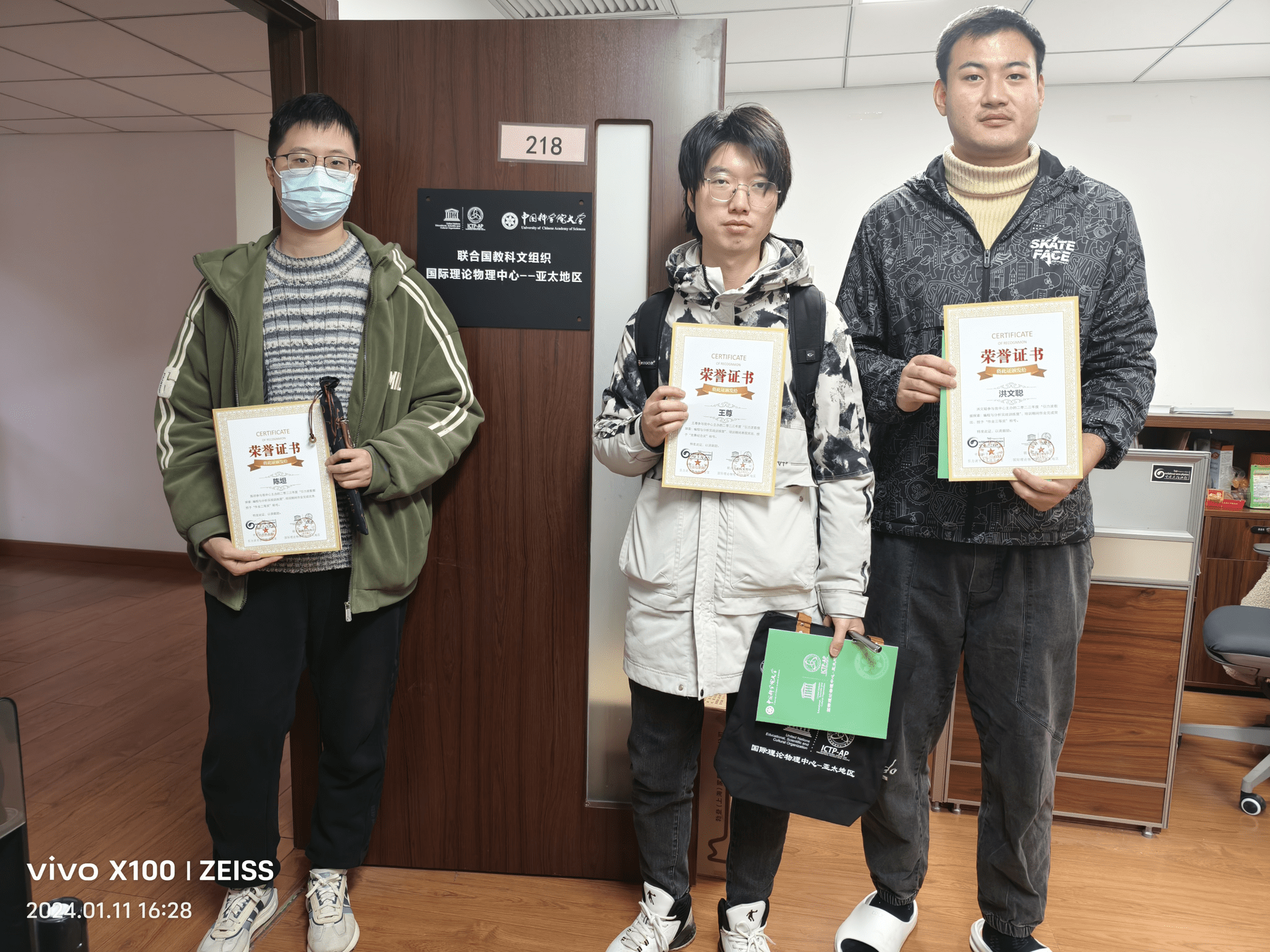
部分获奖同学:
训练营课程回顾与总结
# GWData: Bootcamp
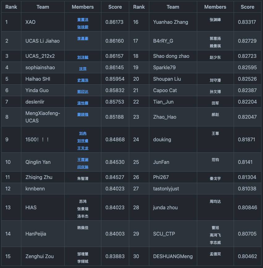
- 竞赛排名情况
-
概述
-
欢迎参加“引力波数据探索:编程与分析实战训练营”系列课程的最后挑战 - “你能找到引力波信号吗?”Kaggle数据科学竞赛(黑客马拉松)!这个竞赛旨在应用你在整个课程中学到的知识和技能,重点关注引力波数据分析和研究。
-
-
任务目标
-
本次竞赛的目标是开发一个能够准确识别引力波信号的模型。我们将提供一个包含噪声和引力波信号的数据集。你的任务是开发一个能够准确区分两者的模型。
-
-
时间线(7天)
-
本竞赛将于北京时间 2023年12月29日22:00 开始,并于北京时间 2024年1月6日23:59 结束。请确保在截止日期前提交你的解决方案。
-
训练营课程回顾与总结
# GWData: Bootcamp
- 竞赛排名情况
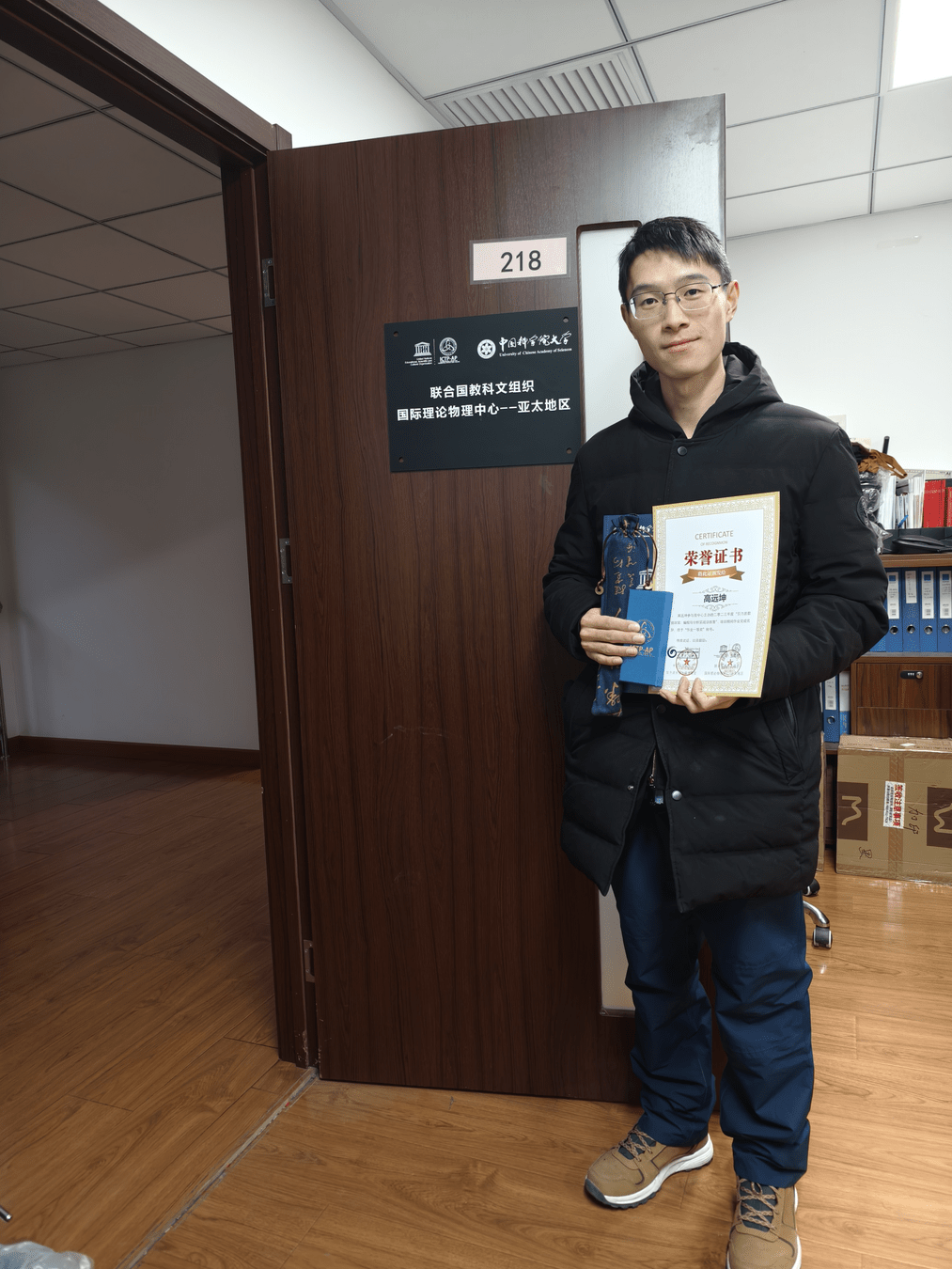
- 作为本次竞赛的冠军,XAO团队展现了非凡的实力。现在让我们有请这个团队的黄震洋同学作为代表,来分享一下他们背后的故事和解题策略。show time!
训练营后记
# GWData: Bootcamp
- 欢迎各类反馈与建议:
记得给课程 Star
- 太极计划引力波物理的最新发展
- 深入数理统计与数据分析的世界
- 全面了解PyTorch系统性课程
- 发现高效科研工具的秘密
- 掌握现代科研方法与学术写作的技巧
- 改善与同学和导师的人际关系
- 学术圈生存的实用指南
- 探索卷的动力学原理
- 寻求自我实现的途径
- 如何找到适合自己的人生方向
- 见到我,记得和我打招呼,期待交流与反馈