Fundamentals of AI/ML and LLMs for Gravitational Wave Search

He WANG [王赫]
2026/08/29 @FQCP2026
ICTP-AP, UCAS

This slides: https://slides.com/iphysresearch/2026aug_fqcp
hewang@ucas.ac.cn

-
Who Am I
— A quick intro and how I got into this field -
What Is Machine Learning?
— The basics and why it matters -
Deep Learning: When Machines Start to See and Think
— From neural networks to powerful representations -
Gravitational Waves Meet Machine Learning
— How ML is reshaping data analysis in GW astronomy -
Let’s Get Practical: Searching for Gravitational Waves
— A hands-on look at applying ML in real GW searches -
LLMs for Gravitational Waves: My Ongoing Work
— Towards automated and interpretable scientific discovery
Content

-
What Is Machine Learning?
— The basics and why it matters -
Deep Learning: When Machines Start to See and Think
— From neural networks to powerful representations -
Gravitational Waves Meet Machine Learning
— How ML is reshaping data analysis in GW astronomy -
Natural Language Processing
— From transformer to three model families -
From Large Language Models to AI Agents
— Why are LLMs so powerful for automated scientific reasoning? -
Can AI Really Discover?
— From interpolation to search, verification, and science -
Harness Engineering for AI Agents
— How to utilize Claude Code, Codex, ...
Content

# Who am I
Who Am I

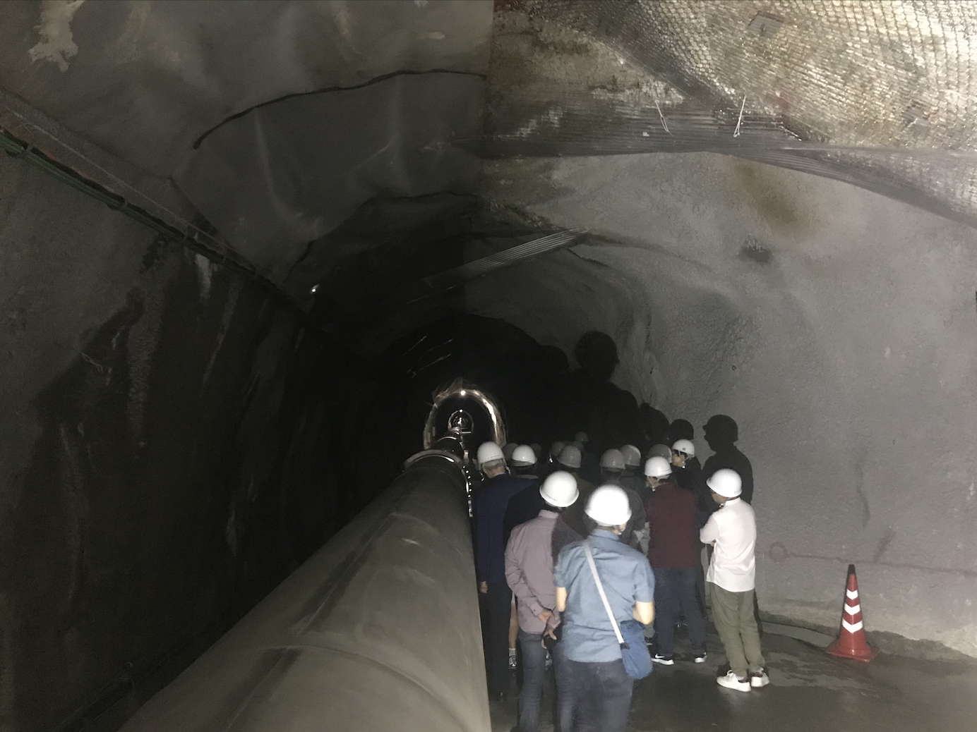
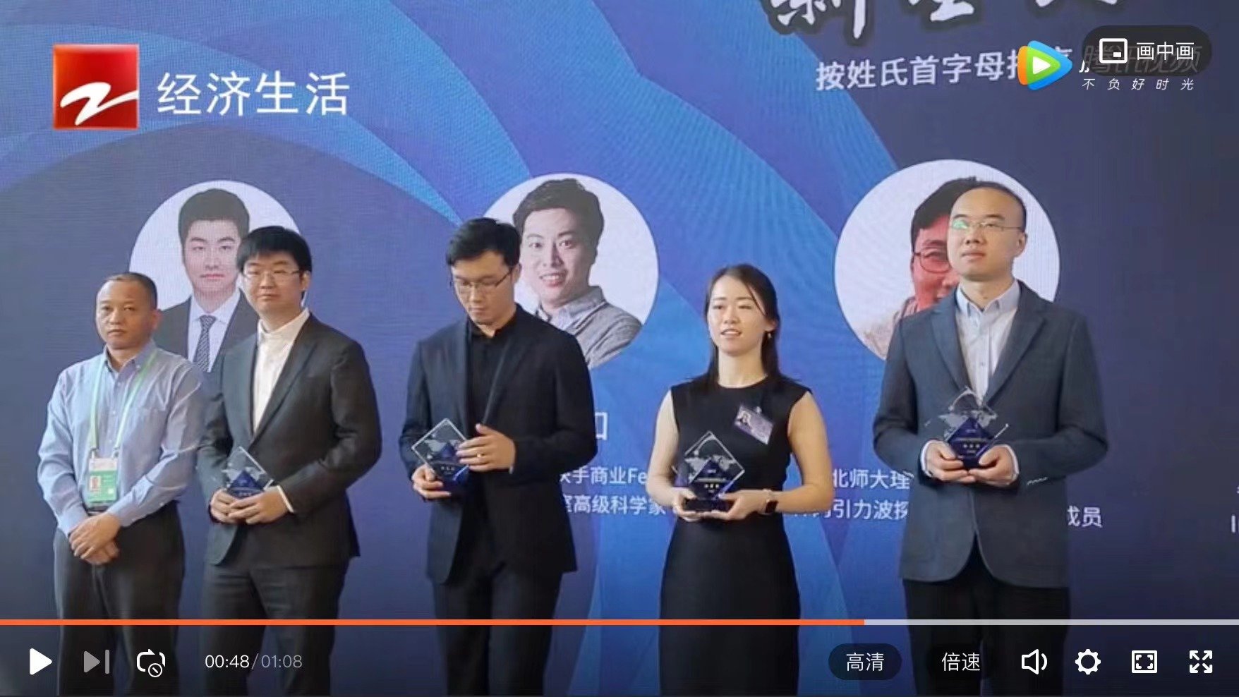
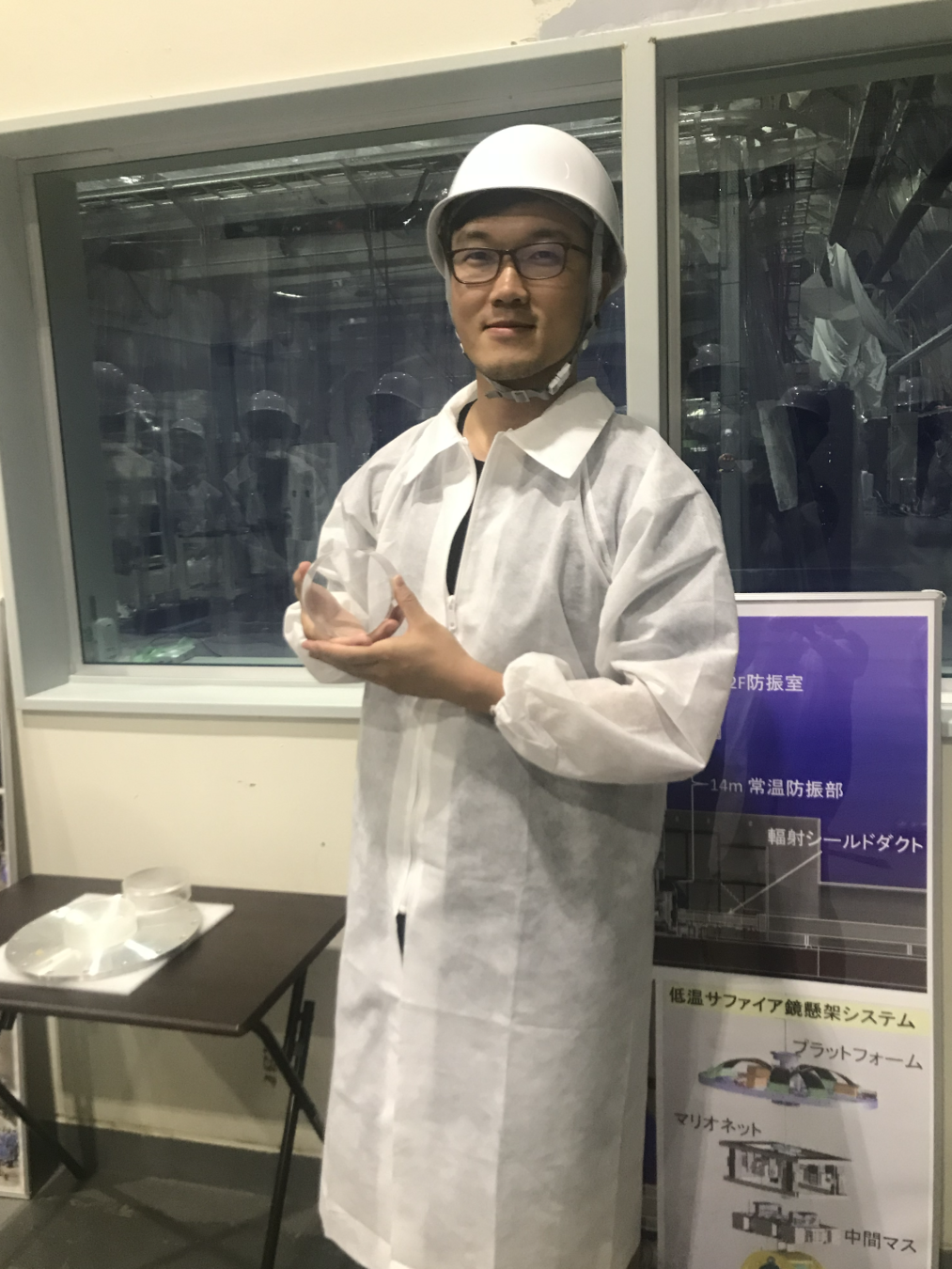
He Wang received his Ph.D. in Theoretical Physics from Beijing Normal University in 2020.
He is currently an Associate Researcher (E-Series) at the ICTP-AP, UCAS. After completing his Ph.D., he conducted postdoctoral research at the ITP-CAS, the Peng Cheng National Laboratory (as a visiting scholar), and UCAS.
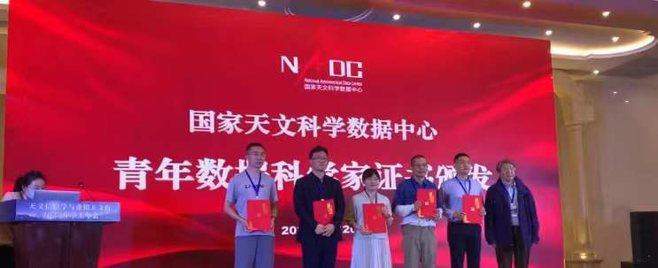
He serves as the Co-chair of the LVK Machine Learning Algorithms (MLA) Group, a Core Member of the LISA Consortium, and a Youth Data Scientist at the National Astronomical Data Center (NADC). As a core contributor to China’s Taiji Program for Space Gravitational Wave Detection, his work focuses on scientific data analysis and algorithmic development.
- GitHub: github.com/iphysresearch
- Blog: IPhysResearch.github.io
Selected Lectures
- Jan 2024
- Aug 2023
-
Machine learning and GW data analysis @TianQin Center
-
Selected Works
- HW, LZ. "Automated Algorithmic Discovery for Gravitational-Wave Detection via LLM-Informed Evolutionary Monte Carlo Tree Search". e-Print: arXiv:2508.03661 [cs.AI]
- HW, et al. “WaveFormer:Transformer-Based Denoising Method for Gravitational- Wave Data.” Mach. learn.: sci. technol. 5, no. 1 (March 2024): 015046. e-Print: arXiv:2212.14283 [gr-qc]
- HW, et al. "Sampling with prior knowledgefor high-dimensional gravitational wave data analysis." Big Data Mining and Analytics 5.1 (2021):53-63.
- HW, et al. "Gravitational-wave signalrecognition of LIGO data by deep learning”. PRD 101 (2020) 10, 104003, e-Print: arXiv:1909.13442 [gr-qc]
Content

-
What Is Machine Learning?
— The basics and why it matters -
Deep Learning: When Machines Start to See and Think
— From neural networks to powerful representations -
Gravitational Waves Meet Machine Learning
— How ML is reshaping data analysis in GW astronomy -
Natural Language Processing
— From transformer to three model families -
From Large Language Models to AI Agents
— Why are LLMs so powerful for automated scientific reasoning? -
Can AI Really Discover?
— From interpolation to search, verification, and science -
Harness Engineering for AI Agents
— How to utilize Claude Code, Codex, ...
# GW: ML
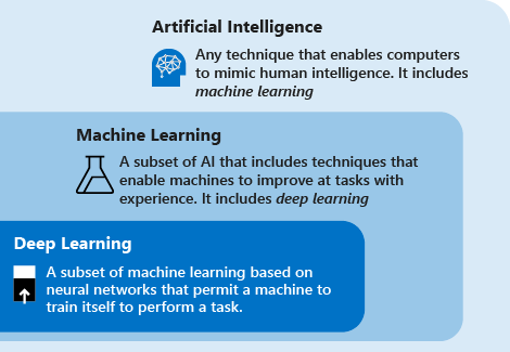
AI \(\supset\) Machine Learning \(\supset\) Deep Learning
-
Machine Learning
-
A major branch of Artificial Intelligence (AI) focused on improving algorithmic performance through learning from experience.
-
Typical models include Linear Regression, Decision Trees, Support Vector Machines (SVMs), and Markov Chain Monte Carlo (MCMC) methods.
-
-
Deep Learning
-
A specialized subfield of machine learning that uses neural networks to automatically extract features from data.
-
Deep neural networks serve as universal function approximators, capable of modeling complex nonlinear mappings.
-
Key characteristics: end-to-end learning, data-driven, and over-parameterized architectures.
-
-
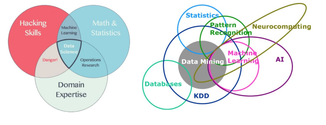
Data-driven approaches: discovering patterns and regularities from data through algorithms and applying them to new data.
Knowledge Discovery in Database, KDD
What Is Machine Learning?
-
“机器学习是对能通过经验自动改进的计算机算法的研究。”
Machine Learning is the study of computer algorithms that improve automatically through experience. -
“机器学习是用数据或以往的经验,以此优化计算机程序的性能标准。”
Machine learning is programming computers to optimize a performance criterion using example data or past experience.
——Alpaydin (2004) -
A computer program is said to learn from experience E with respect to some class of tasks T and performance measure P, if its performance at tasks in T, as measured by P, improves with experience E. ——Tom Mitchell (1997)
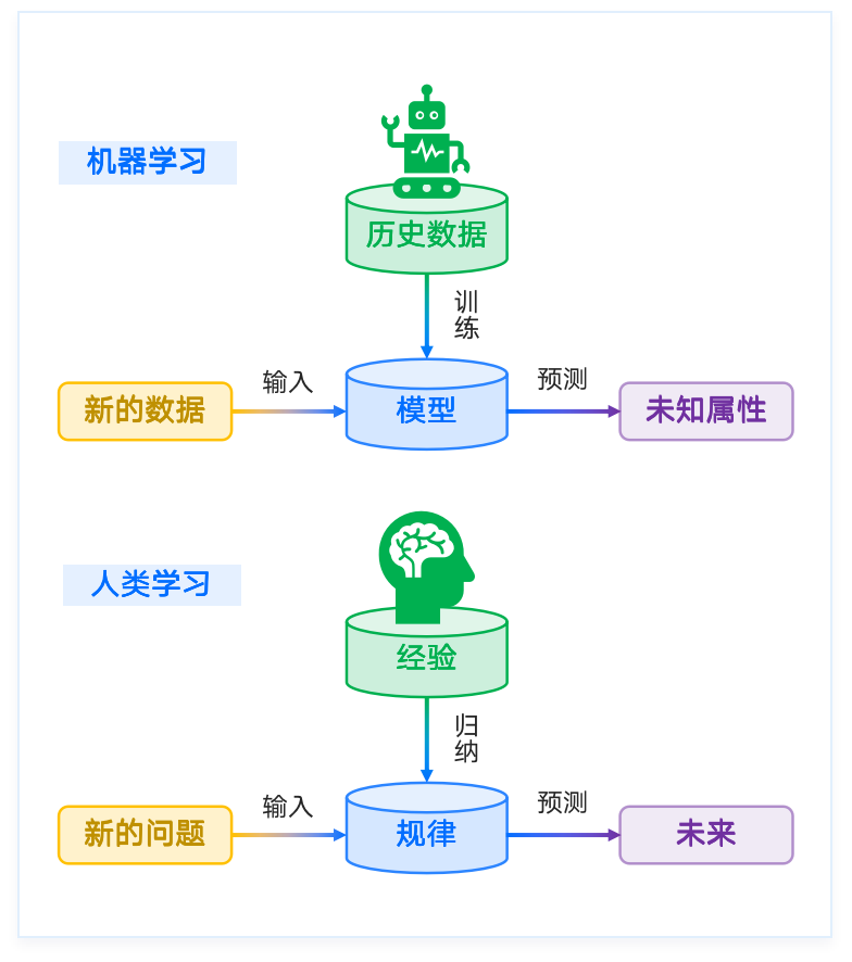
# GW: ML
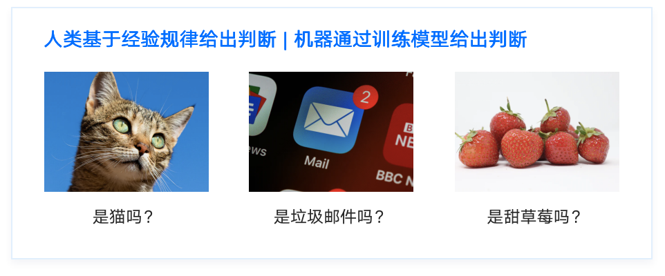
Humans make judgments based on experience —
Machines make judgments by training models on data.
Is it a cat?
Is it a spam?
Is it a sweet
strawberry?
Machine learning
Human learning
experience
data
train
train
input
input
new data
new problem
predict
predict
unknown property
future
Common Types of Machine Learning
# GW: ML
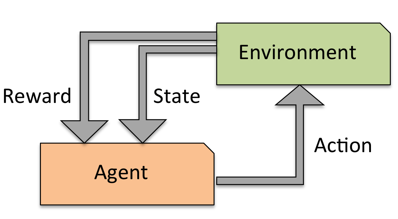
Machine learning models can be broadly categorized based on the presence of labels in training data and how they interact with their environment:
-
Supervised Learning — learning from labeled data
-
Unsupervised Learning — discovering structure in unlabeled data
-
Reinforcement Learning — learning through interaction and feedback from the environment
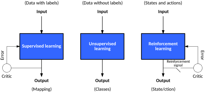
Common Types of Machine Learning: SL
# GW: ML
-
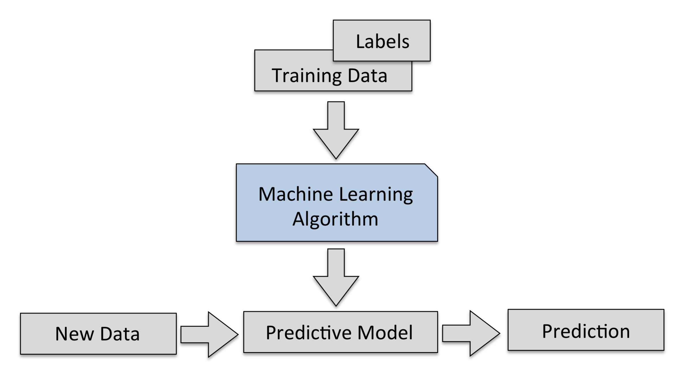
Supervised learning (SL) teaches machines with explicit guidance — the key is that training data are labeled with known outputs (labels).
-
The goal is for the model, after observing labeled training examples (inputs and expected outputs), to predict the correct output for unseen inputs.
-
To achieve this, the model must generalize from the observed data in a meaningful way — a process similar to how humans and animals learn concepts from examples, known as concept learning in cognitive science.
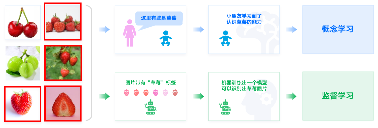
Some of these are strawberries.
The child learns to recognize what a strawberry looks like.
Concept Learning
Images are labeled with “strawberry.”
The machine trains a model that can recognize strawberries.
Supervised Learning
Supervised Learning vs Matched Filtering
# GW: ML
Supervised learning: the key is labeled training data.
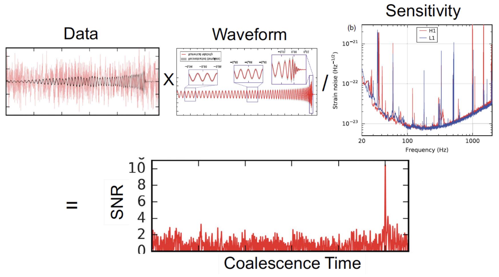
Matched filtering (template-based GW search)
-
Given a segment of time-series data as input, the detection statistic (the matched-filter signal-to-noise ratio over time) is an output time series.
-
The core question: Which linear filter (i.e., which template) maximizes that output?
-
In practice, matched filtering correlates the data with a template waveform and is the optimal linear detector for signals buried in stationary Gaussian noise — it produces the maximum SNR for a given template.
# GW: ML
-
Unsupervised learning (uSL) is a learning process without guidance, where the training data to be learned has no labels.
-
Machine learning algorithms identify common characteristics in the data through certain methods and group data with shared features together. This process is sometimes referred to as "clustering."
-
Clustering involves statistically classifying similar objects into different groups or more subsets so that member objects within the same subset share similar attributes.
-
Unsupervised learning algorithms freely explore the data, and much of what is learned must involve understanding the data itself, rather than applying this understanding to specific tasks. Therefore, mastering unsupervised learning is essential on the path to general intelligence.
-
The process of unsupervised learning is similar to the human process of inductive learning.
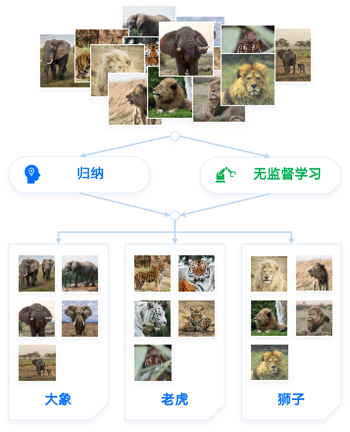
Common Types of Machine Learning: uSL
Unsupervised Learning
Induction
Elephant
Tiger
Lion
# GW: ML
-
Unsupervised learning (uSL) is a learning process without guidance, where the training data to be learned has no labels.
-
Machine learning algorithms identify common characteristics in the data through certain methods and group data with shared features together. This process is sometimes referred to as "clustering."
-
Clustering involves statistically classifying similar objects into different groups or more subsets so that member objects within the same subset share similar attributes.
-
Unsupervised learning algorithms freely explore the data, and much of what is learned must involve understanding the data itself, rather than applying this understanding to specific tasks. Therefore, mastering unsupervised learning is essential on the path to general intelligence.
-
The process of unsupervised learning is similar to the human process of inductive learning.
Common Types of Machine Learning: uSL
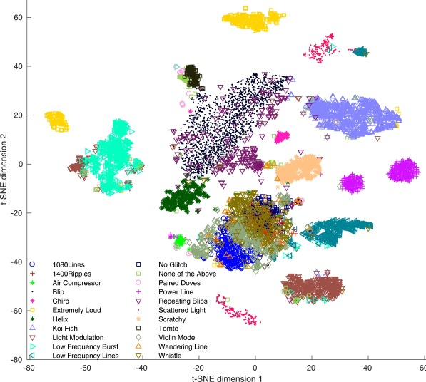
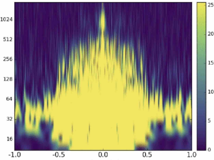
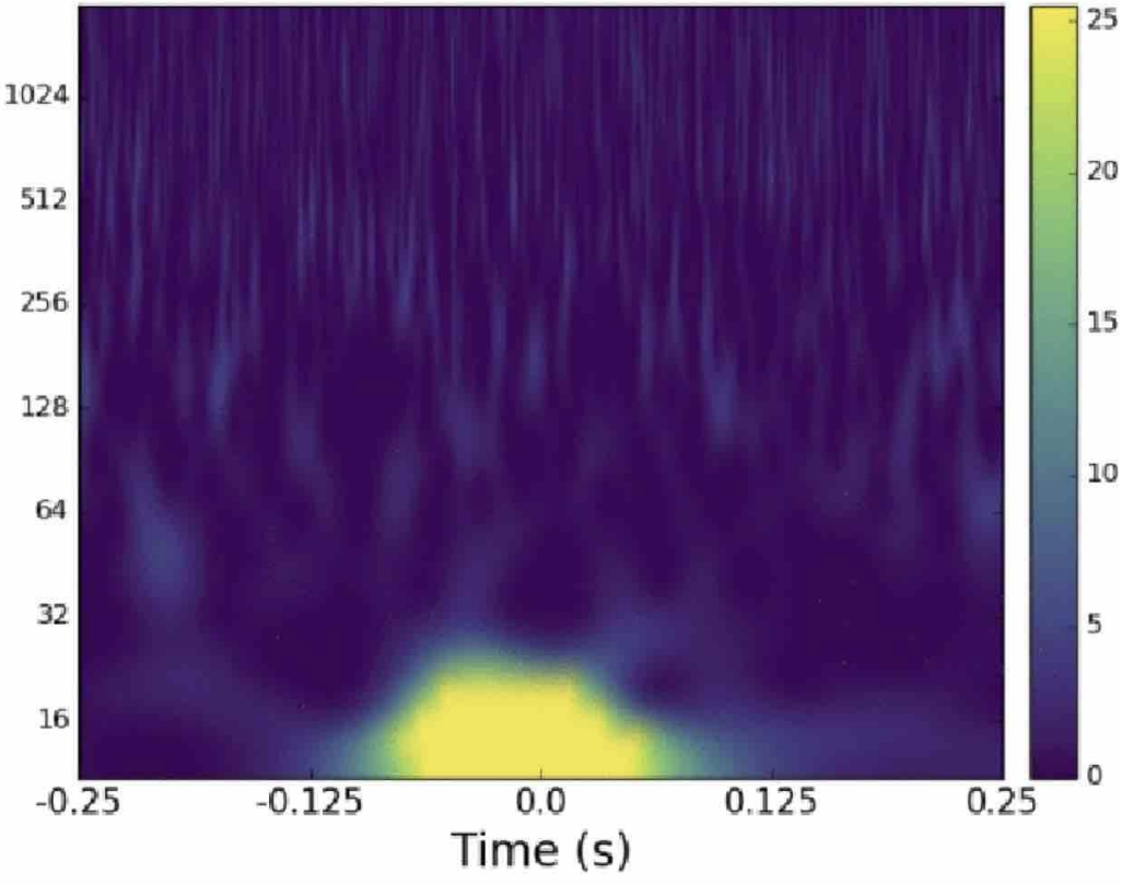
Taxonomy & Categorization of Machine Learning Models
- ML Paradigms & Supervised vs. Unsupervised Learning
- Parametric vs. Non-Parametric Modeling
# GW: ML

Classification of Machine Learning Models
# GW: ML
-
Prediction Based on Supervised Learning
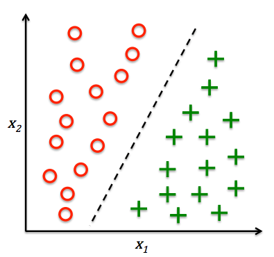
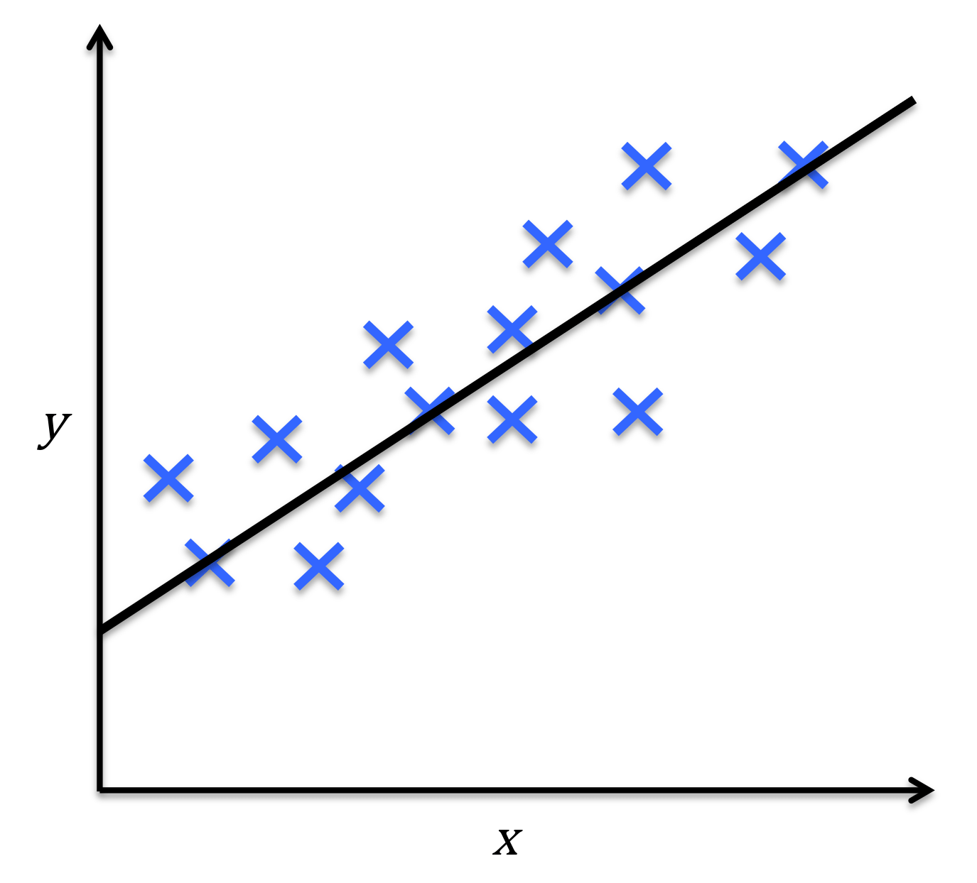
Classification Tasks
(Predicting Different Categories)
Regression Problems (Predicting Continuous Values)
- RL
-
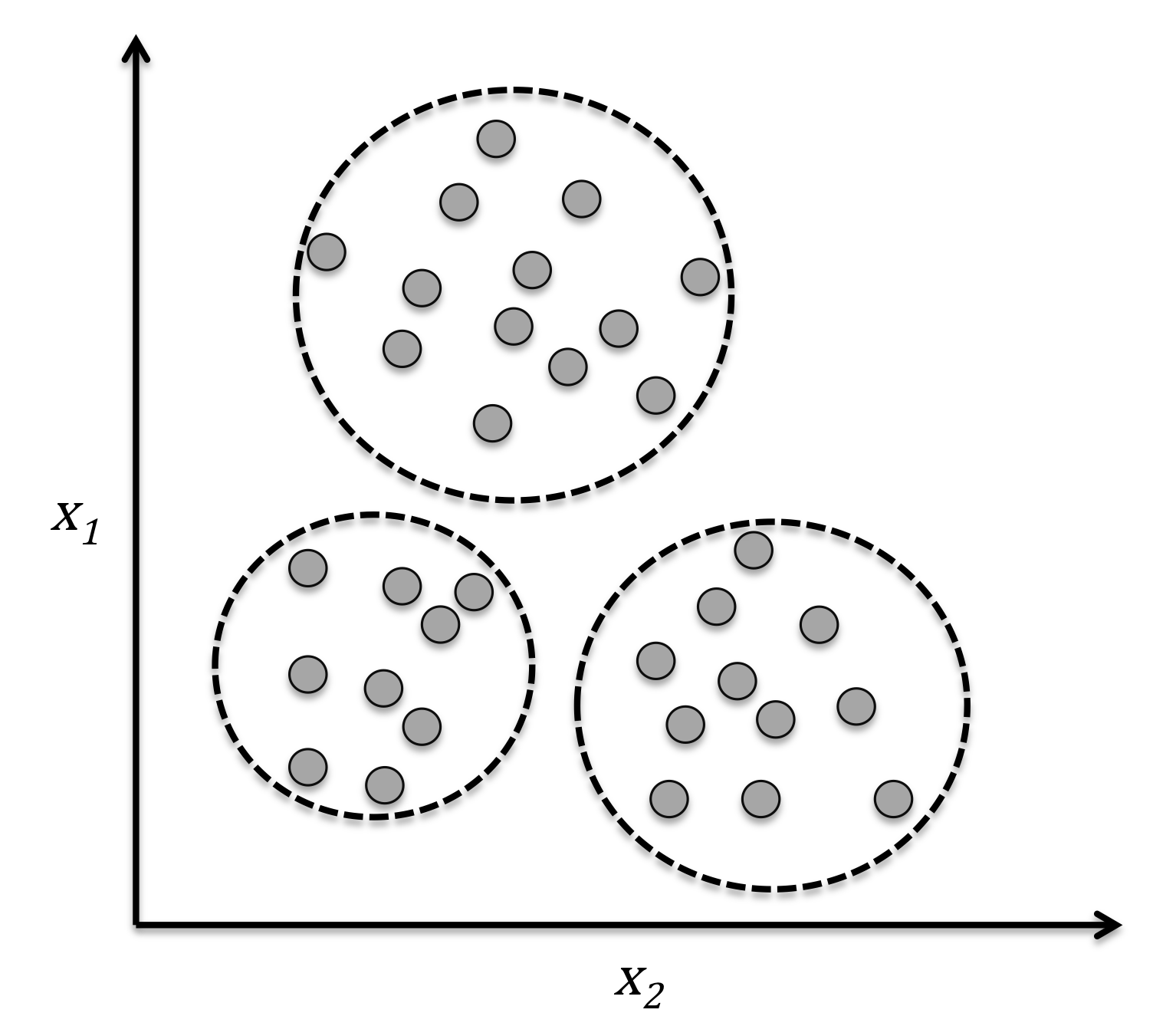
Unsupervised Learning: Extracting Patterns from Unlabeled Data
Use clustering to discover subgroups.
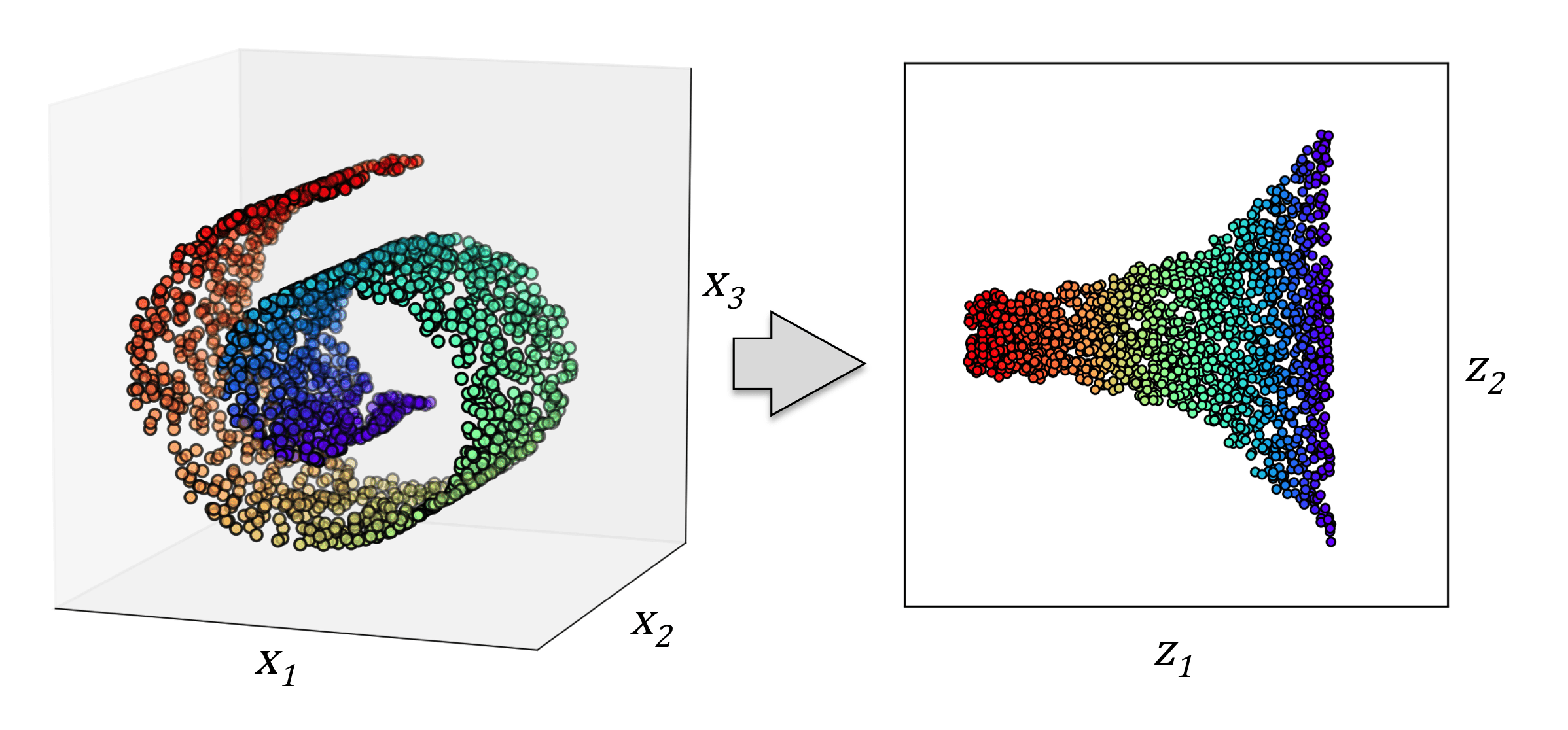
Dimensionality Reduction
Based on the features extracted from data samples, determine which of a finite number of categories they belong to.
Based on the features extracted from data samples, predict continuous value outcomes.
Based on the features extracted from data samples, mine association patterns in the data.
Discover hidden patterns and structures in the data.
# GW: ML
TSNE
UMAP
-
Based on labels
Classification of Machine Learning Models
# GW: ML
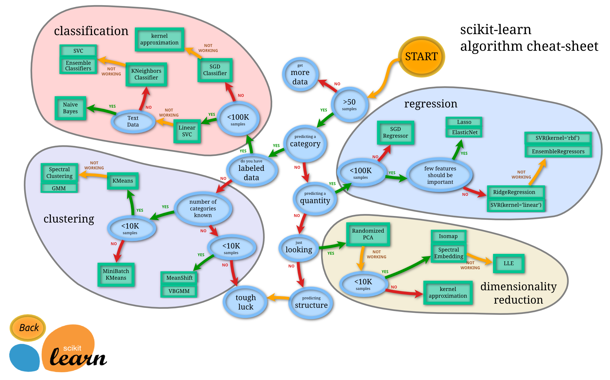
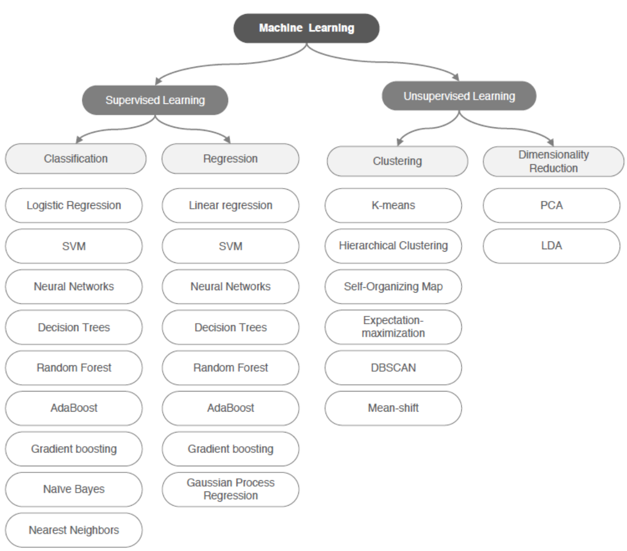
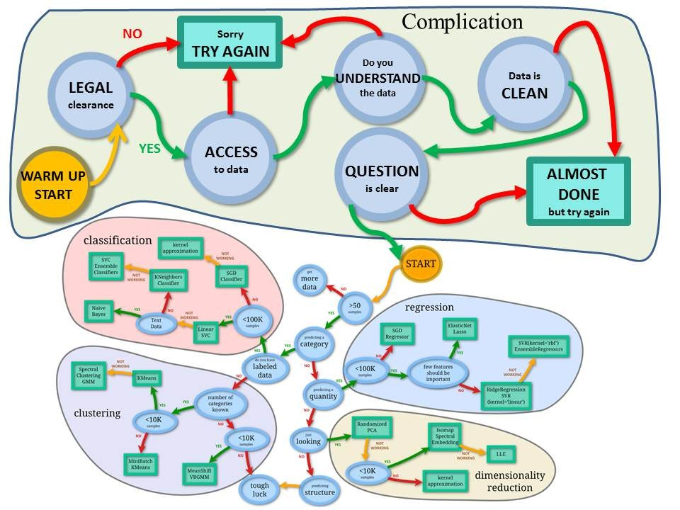
The blue circle contains the judgment criteria, and the green box contains the selectable algorithms. You can find your own operational path based on your data characteristics and task objectives, and just take it step by step.
Classification of Machine Learning Models
-
Based on labels
# GW: ML
Classification of Machine Learning Models
-
Based on labels
Other Types of Machine Learning
# GW: ML
-
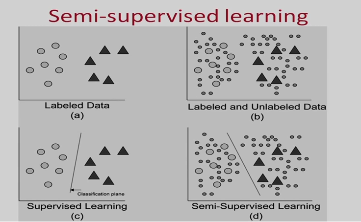
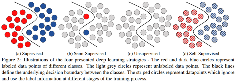
Semi-Supervised Learning (半监督学习)
-
Self-Supervised Learning (自监督学习)
-
...
2002.08721
-
Based on labels
# GW: ML
x
y
y=mx+b
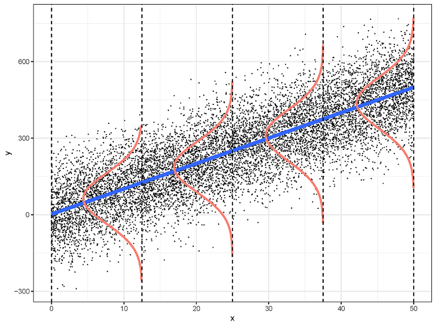
Conditional Probability \(P(Y|X)\) follows a Gaussian distribution
Linear Regression
-
Classification by Data Distribution: Parametric vs. Non-Parametric Models
-
Here, “parametric” does not refer to the parameters within a model, but rather to the parameters of the data distribution itself.
-
-
Parametric Models:
-
Assume a specific form for the data distribution
-
The underlying data patterns or mappings can be described using a finite and fixed set of model parameters.
-
Examples: Linear/Logistic Regression, Perceptron, K-Means Clustering
- Advantages: Simple, fast, and requires less data
- Limitations: Fixed functional form, limited complexity, prone to underfitting
Classification of Machine Learning Models
# GW: ML
x
y
y=mx+b
Conditional Probability \(P(Y|X)\) follows a Gaussian distribution
Linear Regression
-
Classification by Data Distribution: Parametric vs. Non-Parametric Models
-
Here, “parametric” does not refer to the parameters within a model, but rather to the parameters of the data distribution itself.
-
-
Parametric Models:
-
Assume a specific form for the data distribution
-
The underlying data patterns or mappings can be described using a finite and fixed set of model parameters.
-
Examples: Linear/Logistic Regression, Perceptron, K-Means Clustering
- Advantages: Simple, fast, and requires less data
- Limitations: Fixed functional form, limited complexity, prone to underfitting
Note: In some cases, the data may not provide enough information to assume a prior distribution, or the problem itself may not exhibit any clear distributional characteristics.
Classification of Machine Learning Models
# GW: ML
-
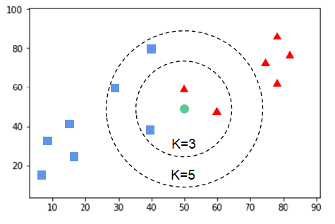
Non-Parametric Models:
-
Make no assumptions about the form of the data distribution; all statistical properties are derived directly from the data.
-
Typically have much higher spatial and temporal complexity than parametric models.
-
Are data-adaptive — the model parameters change dynamically with the samples.
-
x
y
y=mx+b
Conditional Probability \(P(Y|X)\) follows a Gaussian distribution
Linear Regression
K-Nearest Neighbors
-
Classification by Data Distribution: Parametric vs. Non-Parametric Models
-
Here, “parametric” does not refer to the parameters within a model, but rather to the parameters of the data distribution itself.
-
-
Parametric Models:
-
Assume a specific form for the data distribution
-
The underlying data patterns or mappings can be described using a finite and fixed set of model parameters.
-
Examples: Linear/Logistic Regression, Perceptron, K-Means Clustering
- Advantages: Simple, fast, and requires less data
- Limitations: Fixed functional form, limited complexity, prone to underfitting
Examples: Random Forest, Naive Bayes, SVM, Neural Networks
- Advantages: Flexible functional forms, fewer strong assumptions, good fitting ability
- Limitations: Require large datasets, slower computation, prone to overfitting, lower interpretability
Note: In some cases, the data may not provide enough information to assume a prior distribution, or the problem itself may not exhibit any clear distributional characteristics.
Classification of Machine Learning Models

Content
-
What Is Machine Learning?
— The basics and why it matters -
Deep Learning: When Machines Start to See and Think
— From neural networks to powerful representations -
Gravitational Waves Meet Machine Learning
— How ML is reshaping data analysis in GW astronomy -
Natural Language Processing
— From transformer to three model families -
From Large Language Models to AI Agents
— Why are LLMs so powerful for automated scientific reasoning? -
Can AI Really Discover?
— From interpolation to search, verification, and science -
Harness Engineering for AI Agents
— How to utilize Claude Code, Codex, ...
The Origins of Deep Learning
# GW: DL
-
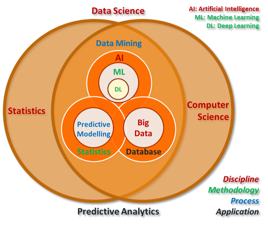
Machine Learning: A key branch of artificial intelligence and an interdisciplinary field
-
Data-Driven: Discovering patterns and regularities from data through algorithms and applying them to new data
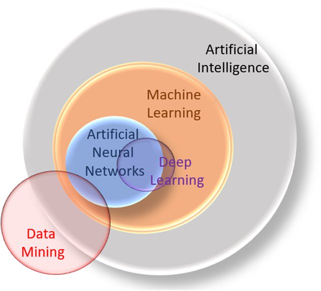
Knowledge Discovery in Database, KDD
# GW: DL
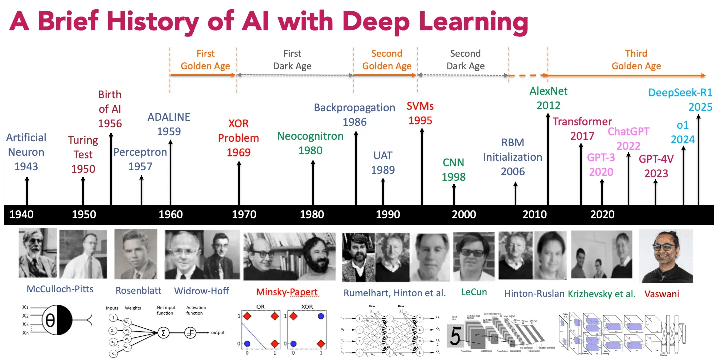
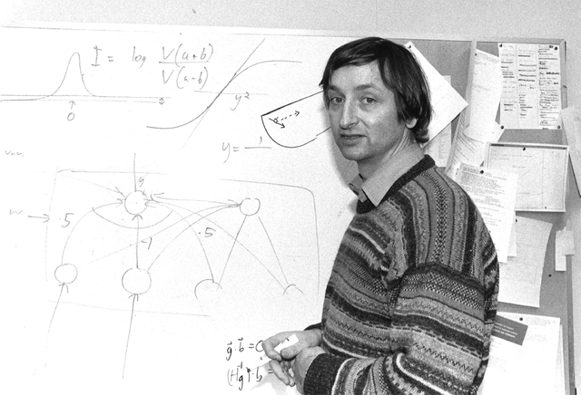
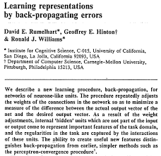
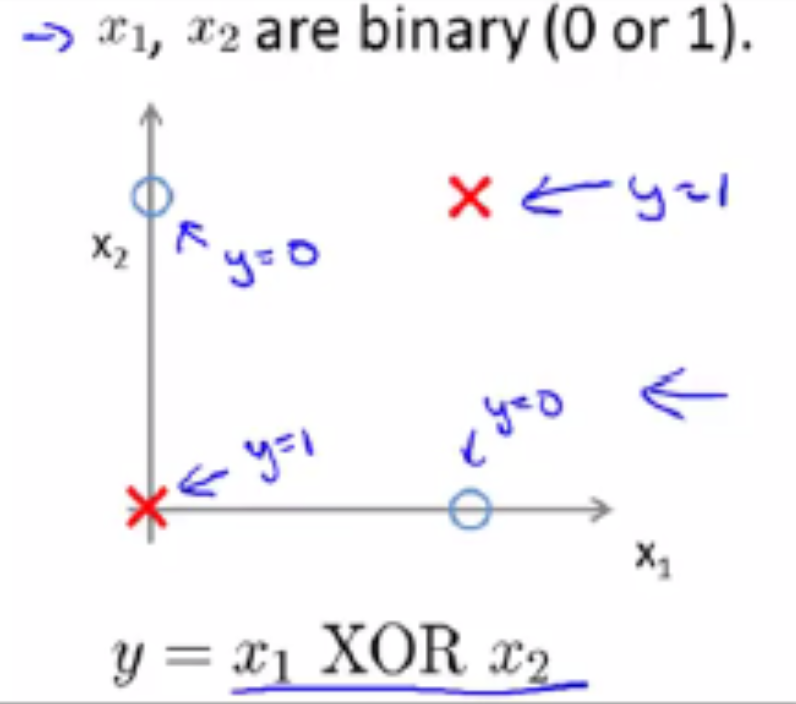
- Milestone Events in the Development of Artificial Intelligence
The Origins of Deep Learning
# GW: DL
- Milestone Events in the Development of Artificial Intelligence
The Origins of Deep Learning
# GW: DL
- Milestone Events in the Development of Artificial Intelligence
The Origins of Deep Learning

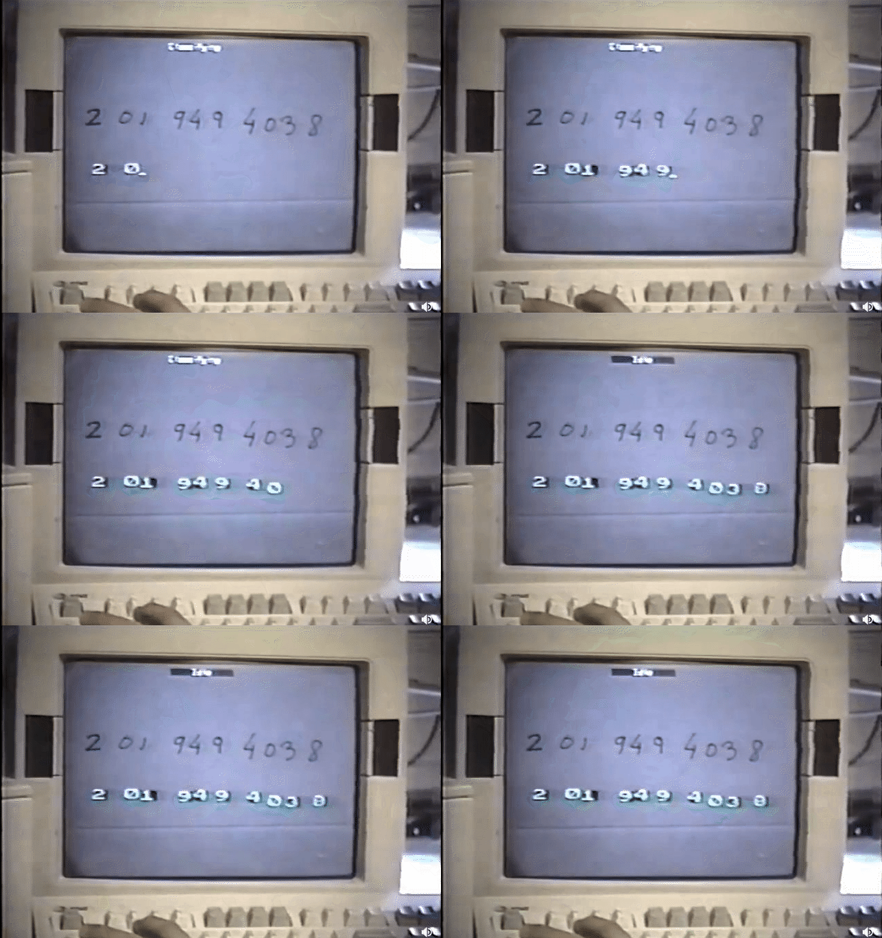
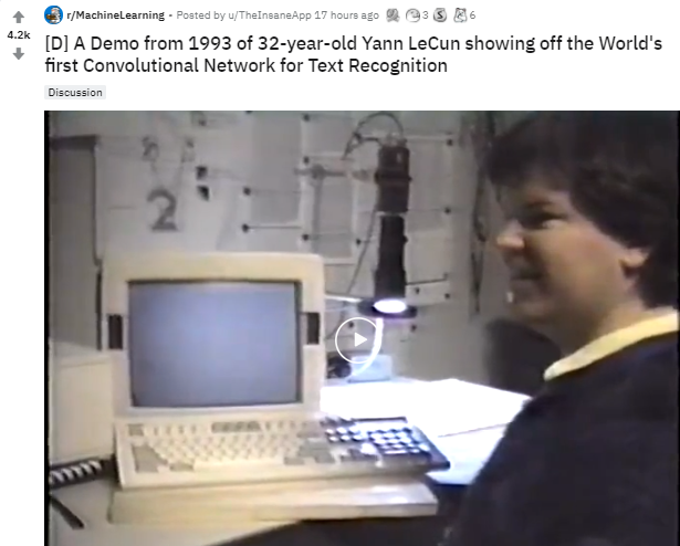
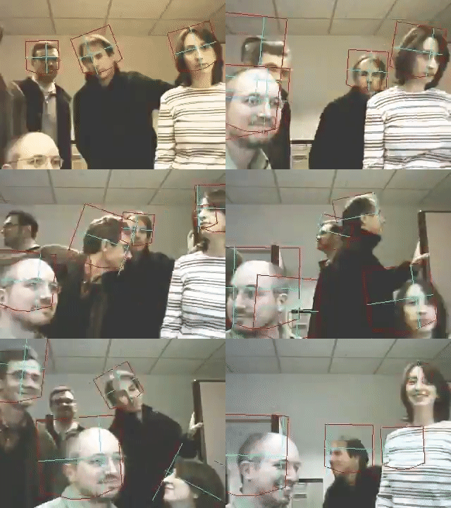
# GW: DL
- Milestone Events in the Development of Artificial Intelligence
The Origins of Deep Learning

SVM (support vector machines)
# GW: DL
- Milestone Events in the Development of Artificial Intelligence
The Origins of Deep Learning
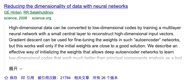

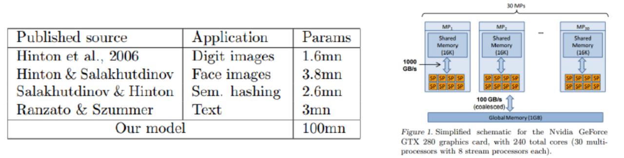
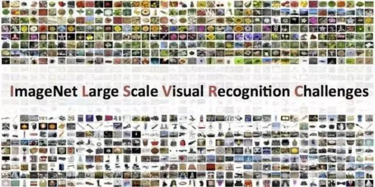
Rajat Raina & Andrew Y. Ng. (ICML09)
(~1970)
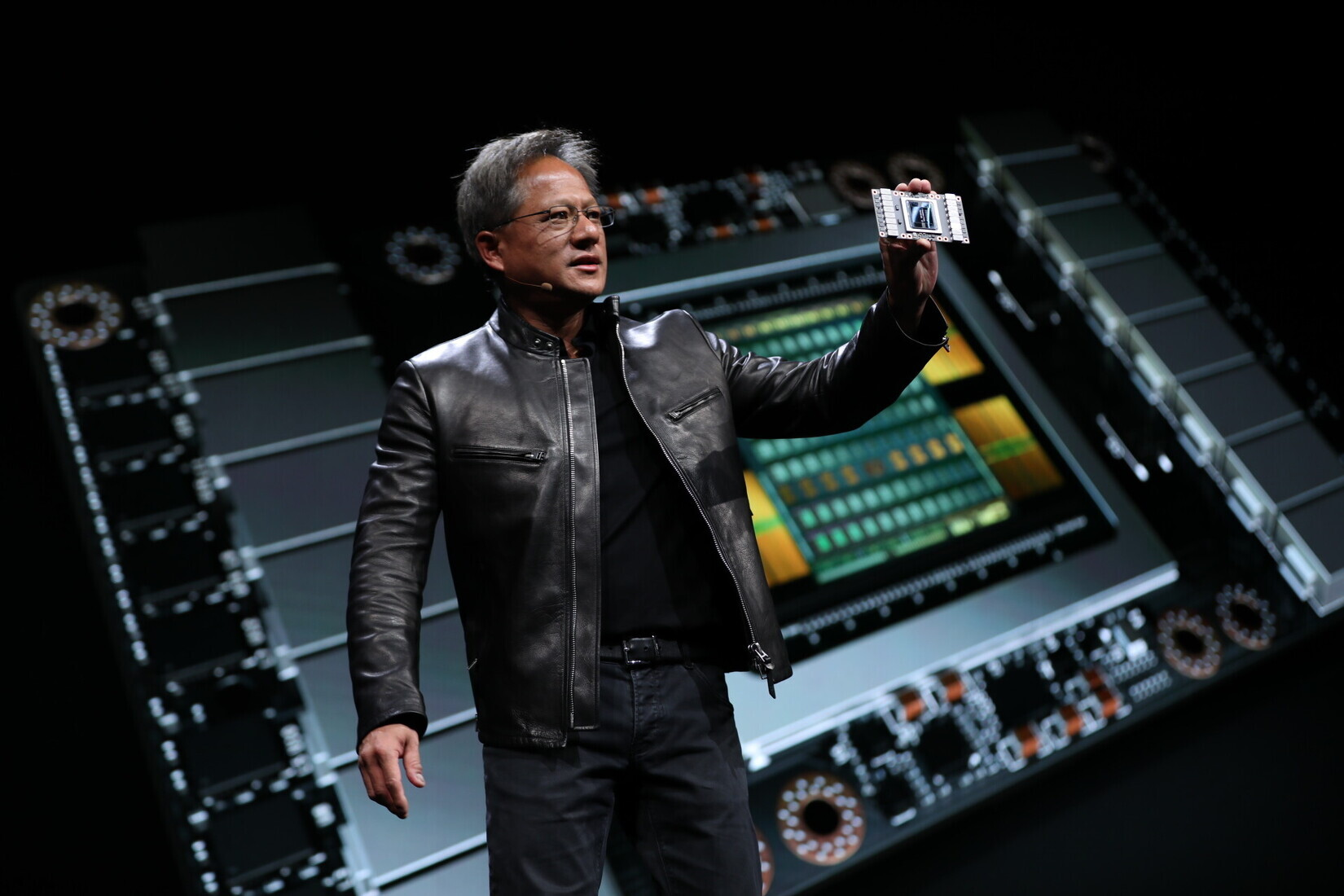
Jen-Hsun Huang.
GPU for DL (~2010)
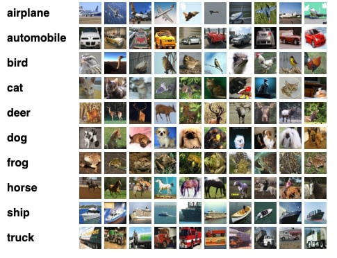
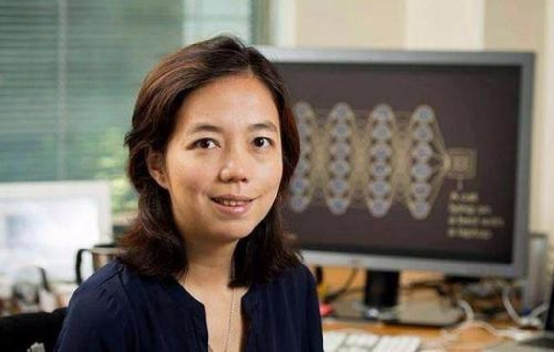
Fei-Fei Li (ILSVRC2010)
# GW: DL
- Milestone Events in the Development of Artificial Intelligence
The Origins of Deep Learning
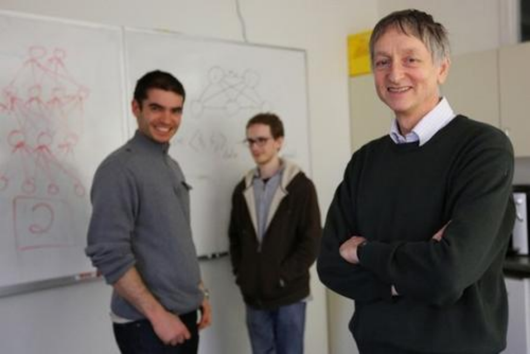
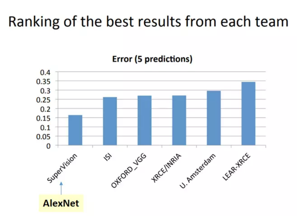
Alex Krizhevsky
Ilya Sutskever
Geoffrey Hinton
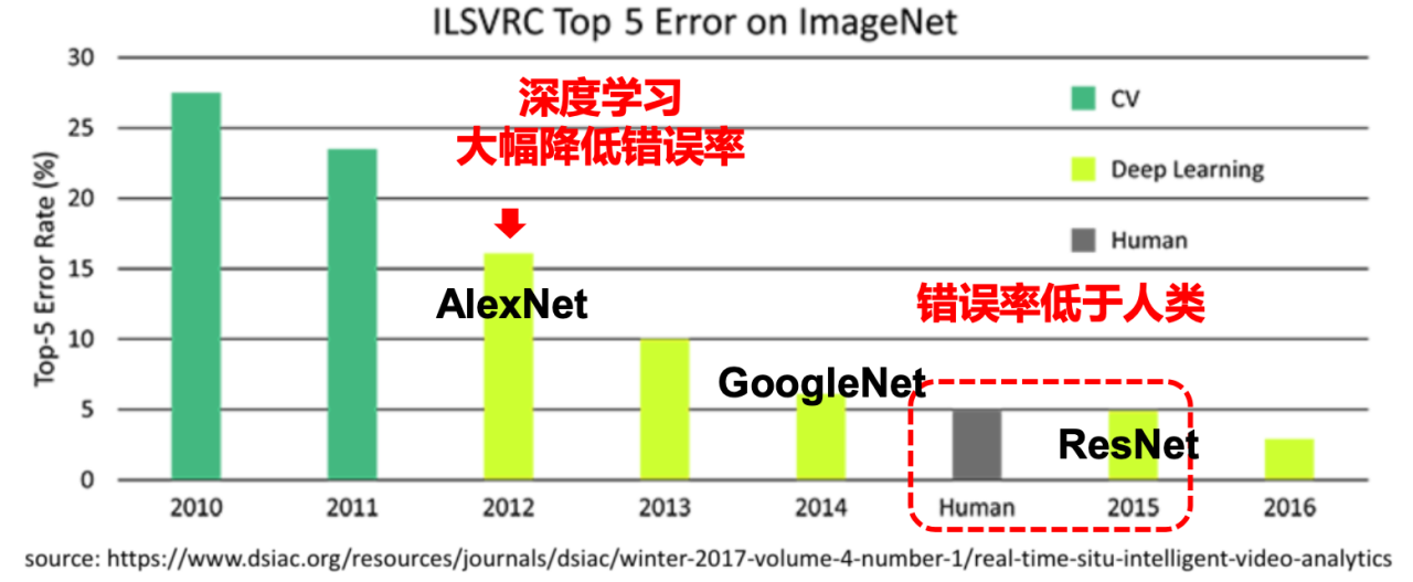
Deep learning
dramatically reduced error rates.
Error rate below human level
The Core of Deep Learning
# GW: DL
- Three Driving Forces of Deep Learning:
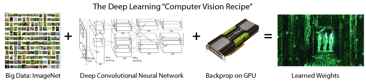
Big Data (Massive scale)
Algorithms
(Neural Networks)
Computing Power (GPU Hardware)
Artificial Intelligence
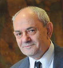
- The Heros of Deep Learning
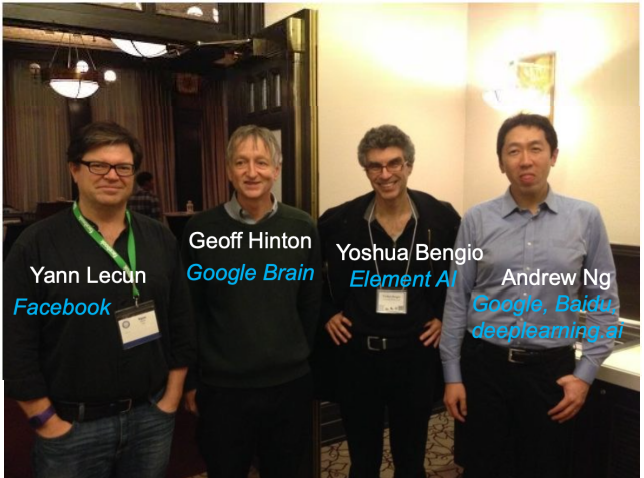
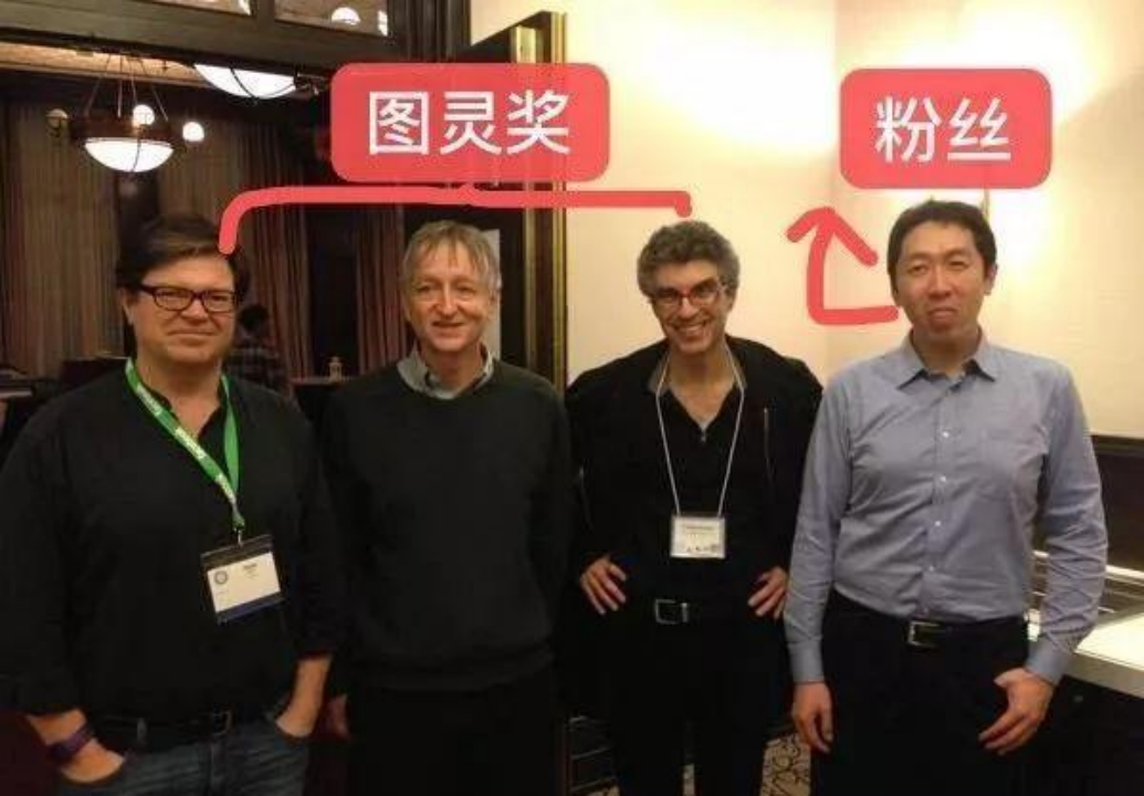
LeCun, Yann, Yoshua Bengio, and Geoffrey Hinton. “Deep Learning.” Nature 521, no. 7553 (May 1, 2015): 436–44. https://doi.org/10.1038/nature14539.

Followers
Turing Award

Geoffrey Hinton
Yoshua Bengio
Yann LeCun
Jen-Hsun Huang
Fei-Fei Li
Bill Dally
The Queen Elizabeth Prize for Engineering
(5th Nov, 2025)
quit?
resigned
Nobel Prize in Physics (2024)
LawZero
+
+
=
Neural Network Mechanics
- Linear transformations ((W x + b))
- activation functions (ReLU, Sigmoid, tanh)
- PyTorch
nn.Linear.
# GW: DL

Characteristics of Deep Learning
# GW: DL
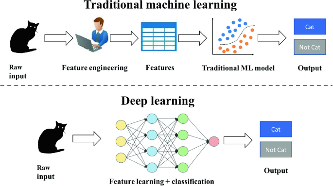
Traditional Machine Learning vs. Deep Learning
- Traditional Machine Learning: Manually designed features
-
In practice, feature design often matters more than the classifier itself.
- Preprocessing: Clean and normalize data, e.g., remove noise or stopwords in text classification.
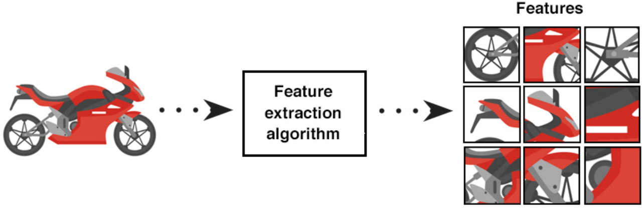
- Feature Extraction: Derive meaningful features from raw data, e.g., edges or scale-invariant features in images.
- Feature Transformation: Modify features, e.g., dimensionality reduction or expansion.
- Feature Selection: Mutual Information, TF-IDF
- Feature Extraction: PCA, SVD, LDA
-
-
Deep Learning: An end-to-end learning paradigm
-
Enables learning of complex nonlinear mappings.
-
Shifts from manual knowledge encoding → learning from data
-
From divide-and-conquer → holistic consideration
-
From algorithm-focused → data-focused
-


LVK. PRD (2021)
What happens in one neuron?
# GW: DL
- Input: A sample
- Input: N samples
- After linear matrix operations, it will go through the activation function to achieve element-wise operations,
making the neurons "non-linear".
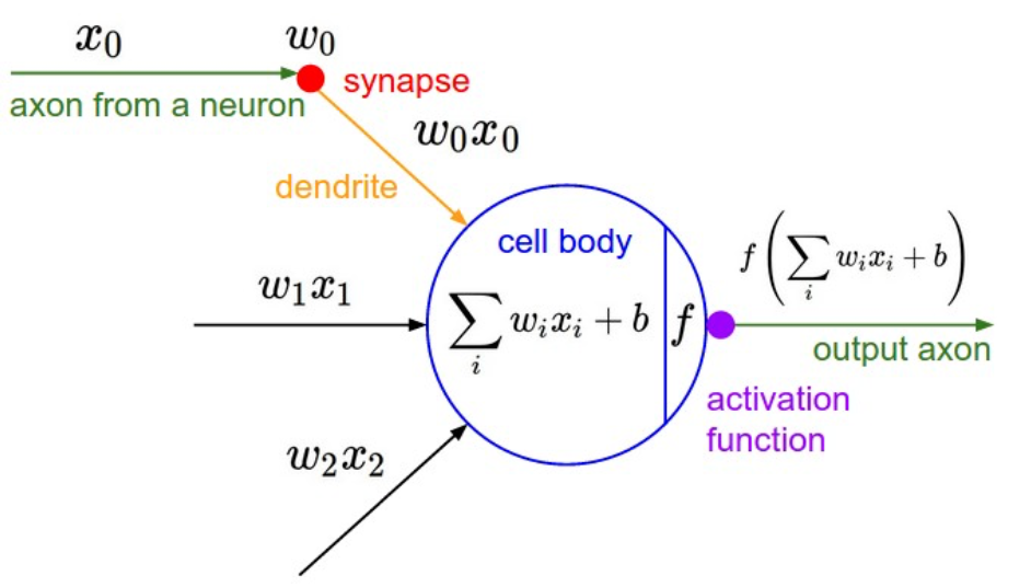
Credit: CS231n
What happens in one neuron?
# GW: DL
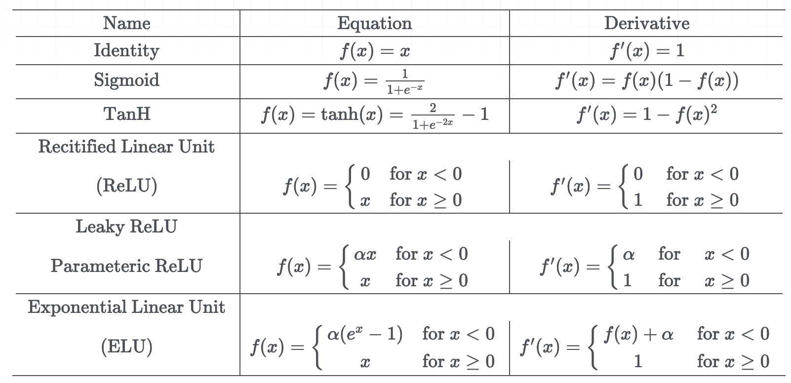
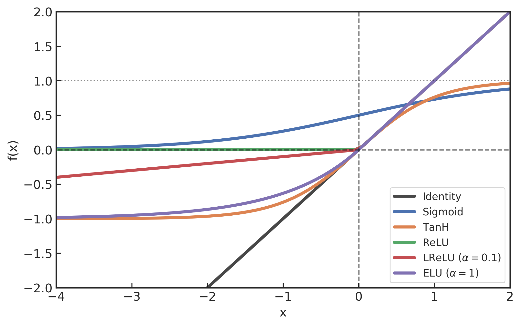
- Activation function \(f\) examples
- S-shaped function (sigmoid)
- ReLU (Rectified Linear Unit)
- S-shaped function (tanh)
- Leaky ReLU
- ELU (Exponential Linear Unit)
- ...
What happens within a layer of neurons?
# GW: DL
- Input: A sample
- Input: N samples (with activation function)
- Note:
- Rows (number of samples) and columns (feature dimensions) of the data matrix
- Rows (corresponding to data feature dimensions) and columns (number of neurons) of a hidden layer
- In the nonlinear mapping process of each layer, the number of rows (samples) in the input and output data matrices remains unchanged
- Over-parameterization neural networks

# GW: DL
-
End-to-End Learning Paradigm:
Deep learning is an automated feature learning approach that can extract useful features directly from raw data. This end-to-end paradigm eliminates the need for manual feature design, enabling the model to learn all the knowledge required to solve a problem directly from the data, greatly enhancing learning capability and efficiency.
Characteristics of Deep Learning
# GW: DL
-
End-to-End Learning Paradigm:
Deep learning is an automated feature learning approach that can extract useful features directly from raw data. This end-to-end paradigm eliminates the need for manual feature design, enabling the model to learn all the knowledge required to solve a problem directly from the data, greatly enhancing learning capability and efficiency.
Characteristics of Deep Learning
# GW: DL
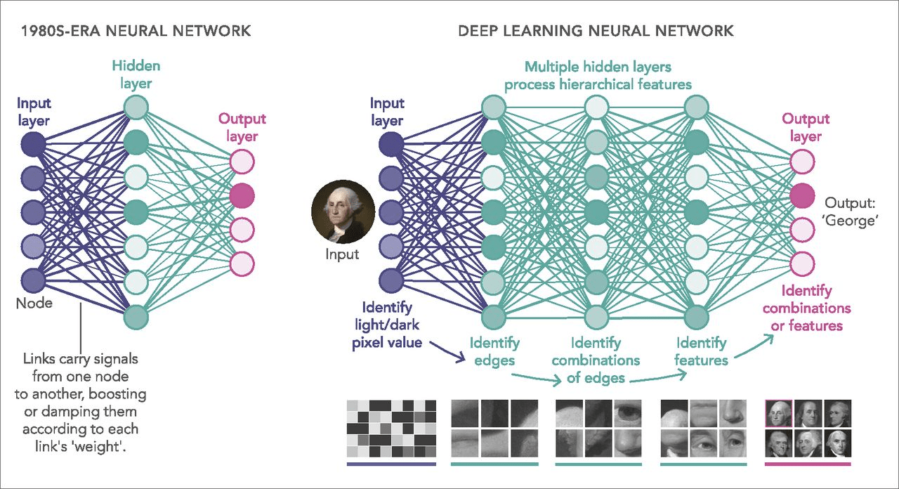
Essence of Deep Learning
# GW: DL
-
Essence: Deep learning uses multi-layer models and large-scale training data (including unlabeled data) to learn more useful features, ultimately improving classification or prediction accuracy.
The deep model is the means; feature learning is the goal. -
Differences from Shallow Learning:
-
Emphasizes model depth, typically with 5–10+ hidden layers;
-
Highlights feature learning: through layer-by-layer transformations, raw features are mapped into new feature spaces, making classification or prediction easier. Compared to manually designed features, learning from large-scale data better captures the rich intrinsic information of the data.
-
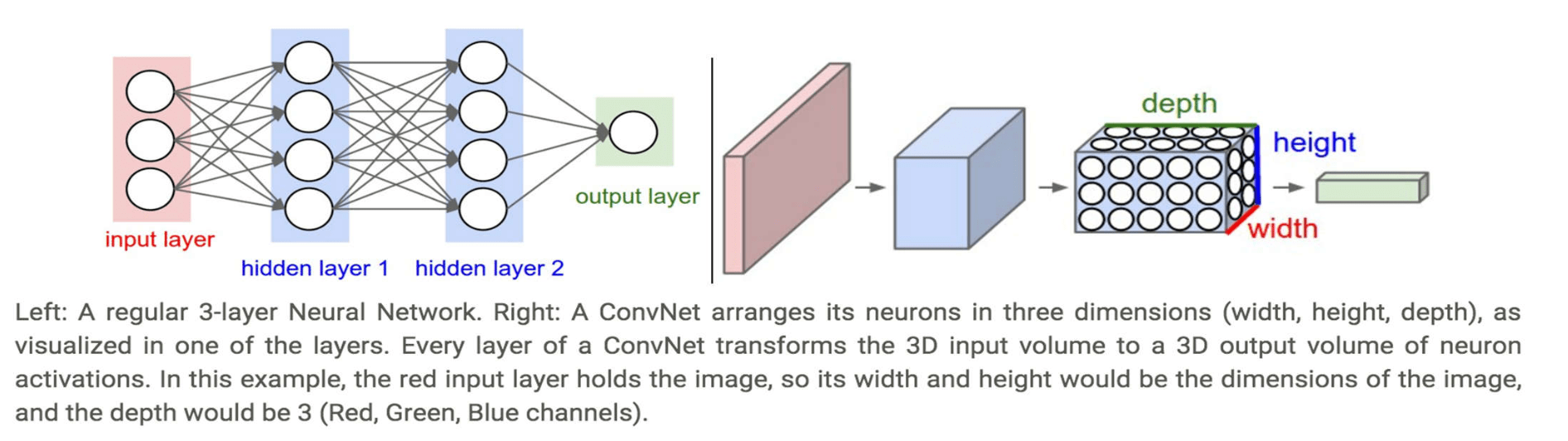
Credit: CS231n
Content
-
What Is Machine Learning?
— The basics and why it matters -
Deep Learning: When Machines Start to See and Think
— From neural networks to powerful representations -
Gravitational Waves Meet Machine Learning
— How ML is reshaping data analysis in GW astronomy -
Natural Language Processing
— From transformer to three model families -
From Large Language Models to AI Agents
— Why are LLMs so powerful for automated scientific reasoning? -
Can AI Really Discover?
— From interpolation to search, verification, and science -
Harness Engineering for AI Agents
— How to utilize Claude Code, Codex, ...
# GW
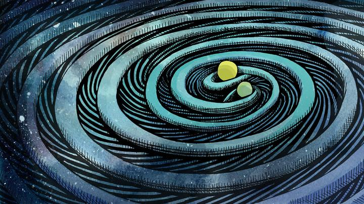
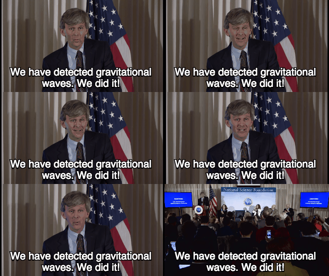
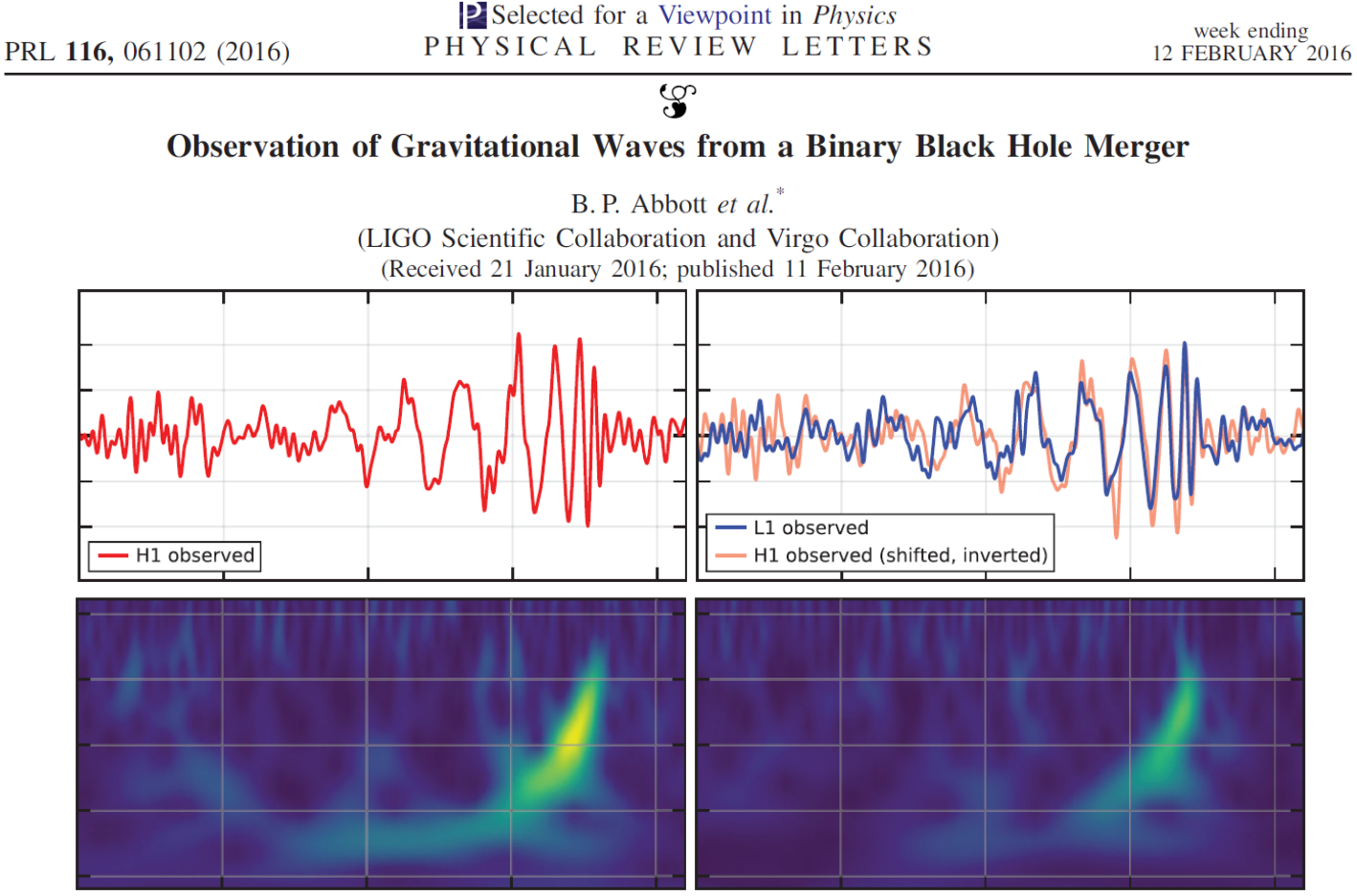
Gravitational waves (GW) are a strong field effect in General Relativity, ripples in the fabric of spacetime caused by accelerating massive objects.
Gravitational Wave Astronomy

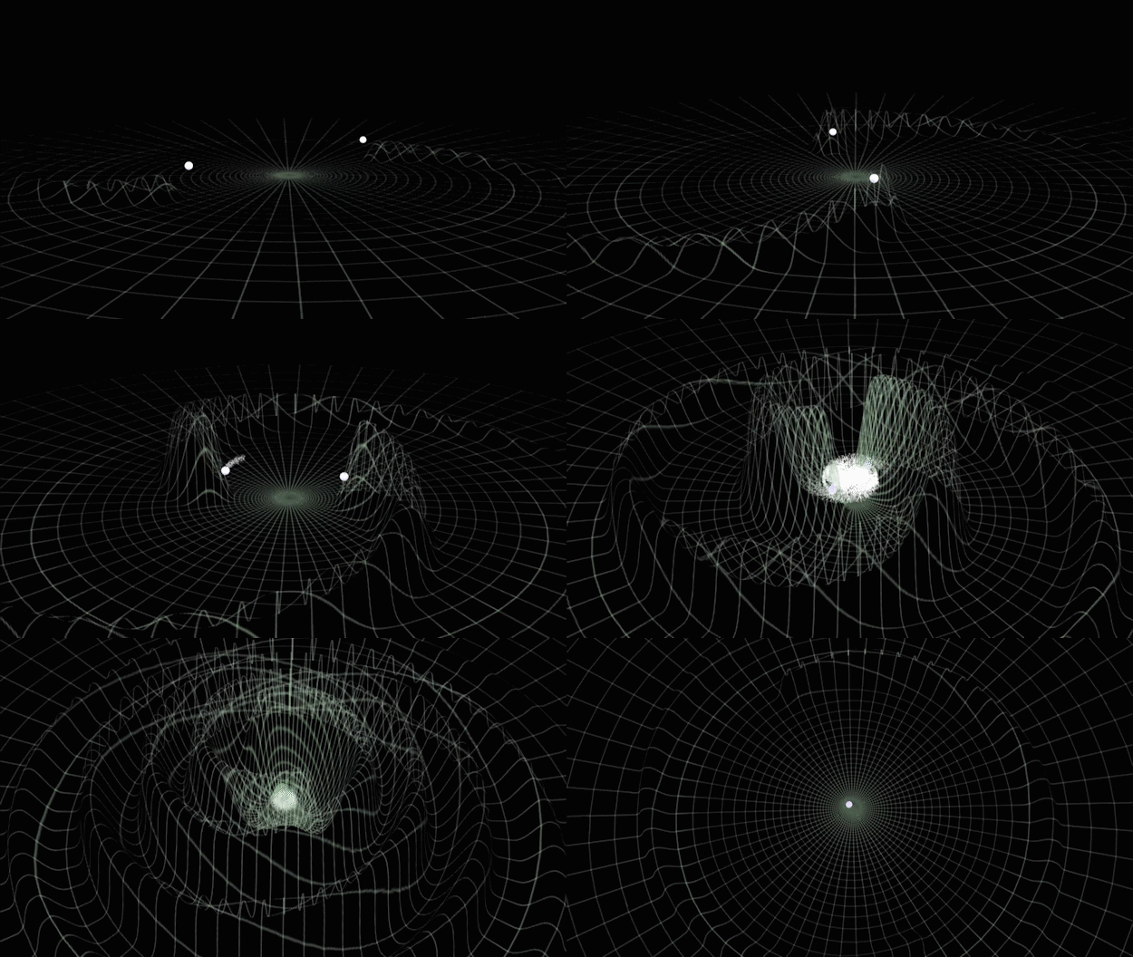
Compact Binary Coalescences
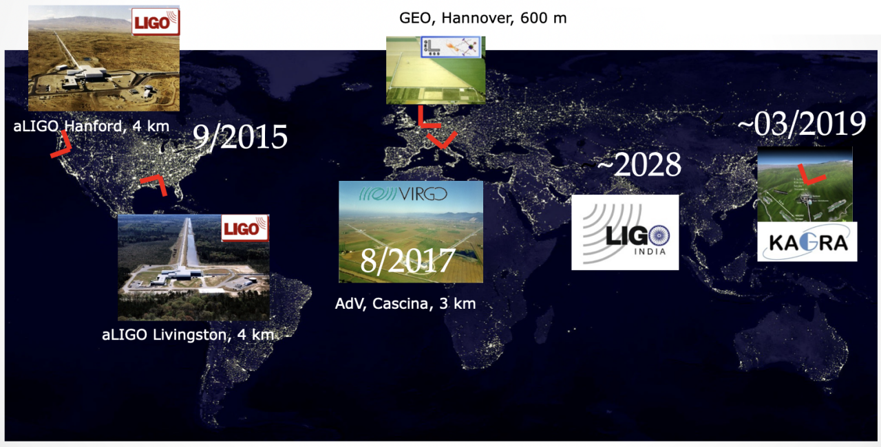
LIGO-Virgo-KAGRA-...
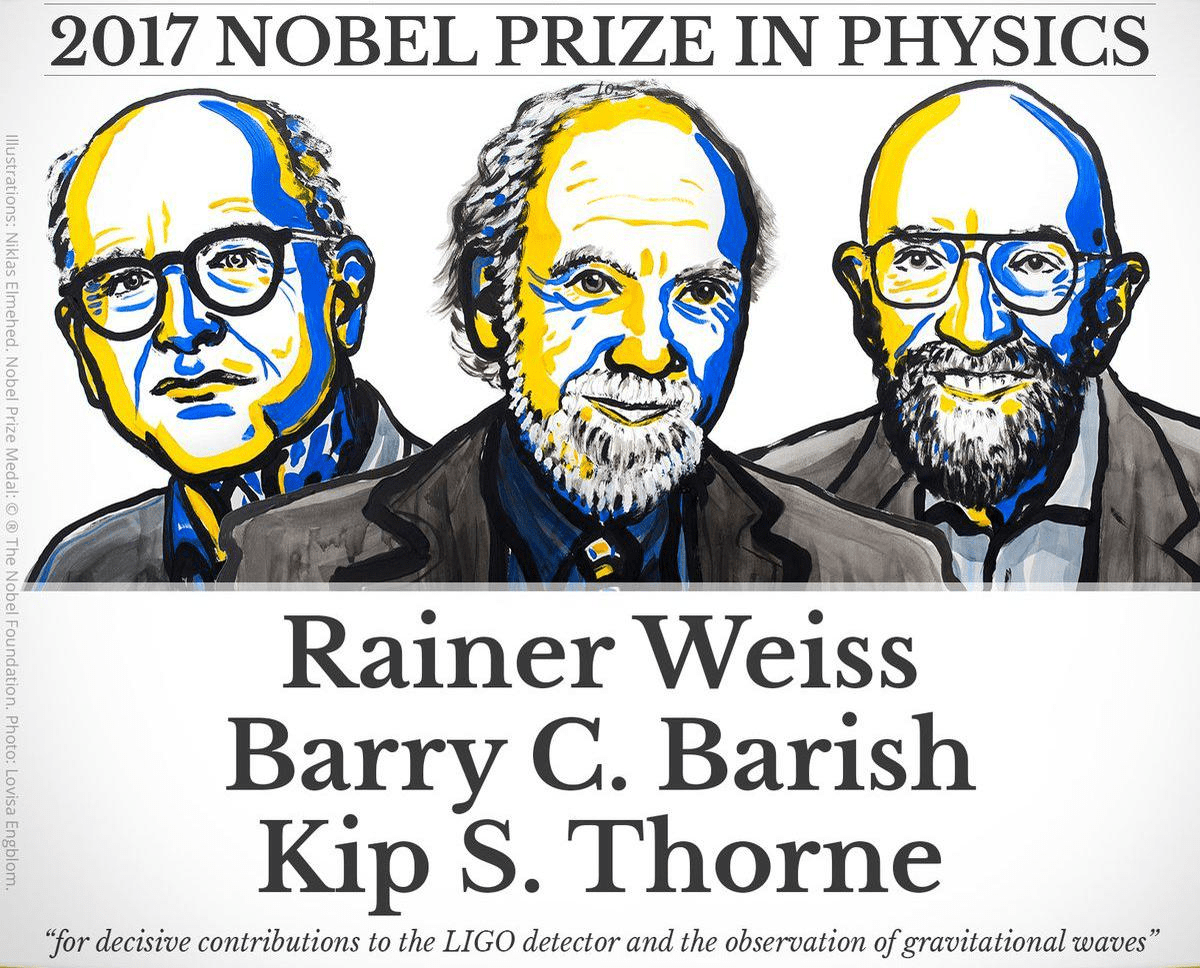
- Detecting gravitational waves require a mix of FIVE key ingredients:
- good detector technology
- good waveform predictions
- good data analysis methodology and technology
- coincident observations in several independent detectors
- coincident observations in electromagnetic astronomy
—— Bernard F. Schutz
DOI: 10.1063/1.1629411
# GW
GW Data Characteristics
LIGO-VIRGO-KAGRA
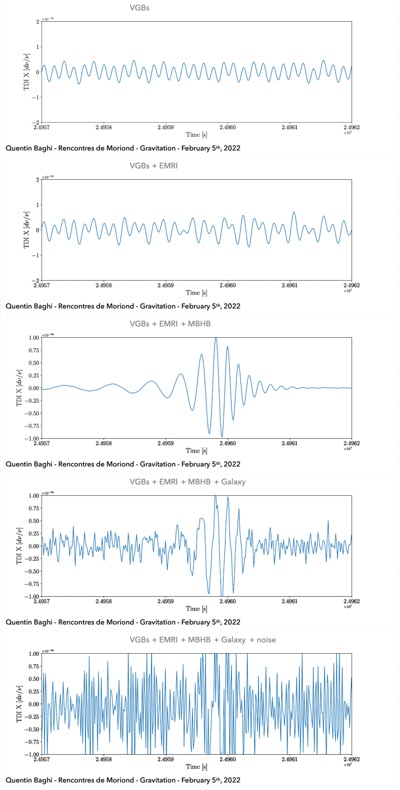
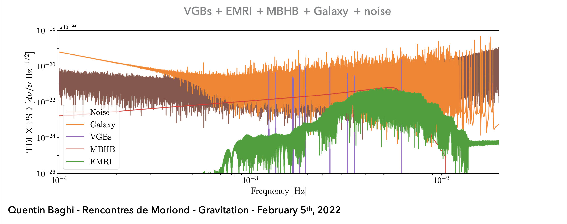
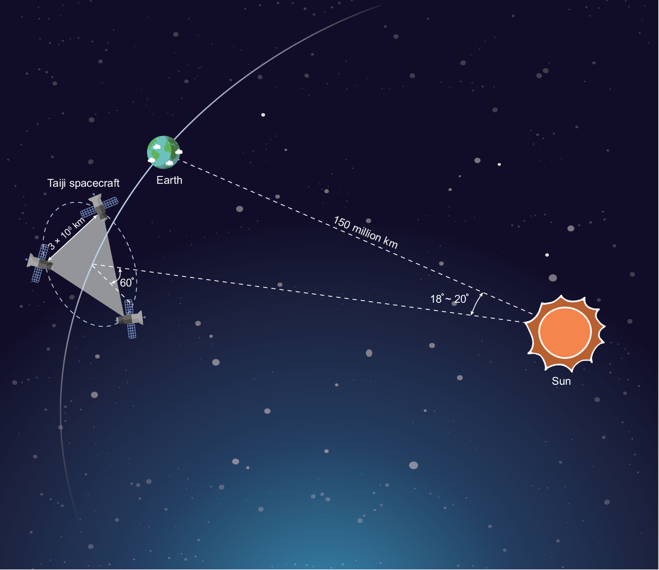
LISA Project
-
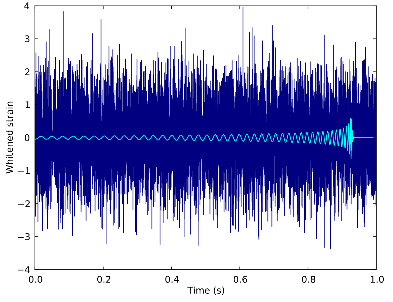
Noise: non-Gaussian and non-stationary
-
Signal challenges:
-
(Earth-based) A low signal-to-noise ratio (SNR) which is typically about 1/100 of the noise amplitude (-60 dB).
-
(Space-based) A superposition of all GW signals (e.g.: 104 of GBs, 10~102 of SMBHs, and 10~103 of EMRIs, etc.) received during the mission's observational run.
-

Matched Filtering Techniques (匹配滤波方法)
-
In Gaussian and stationary noise environments, the optimal linear algorithm for extracting weak signals
- Works by correlating a known signal model \(h(t)\) (template) with the data.
- Starting with data: \(d(t) = h(t) + n(t)\).
- Defining the matched-filtering SNR \(\rho(t)\):
\(\rho^2(t)\equiv\frac{1}{\langle h|h \rangle}|\langle d|h \rangle(t)|^2 \) , where
\(\langle d|h \rangle (t) = 4\int^\infty_0\frac{\tilde{d}(f)\tilde{h}^*(f)}{S_n(f)}e^{2\pi ift}df \) ,
\(\langle h|h \rangle = 4\int^\infty_0\frac{\tilde{h}(f)\tilde{h}^*(f)}{S_n(f)}df \),
\(S_n(f)\) is noise power spectral density (one-sided).
Statistical Approaches
Frequentist Testing:
- Make assumptions about signal and noise
- Write down the likelihood function
- Maximize parameters
- Define detection statistic
→ recover MF
Bayesian Testing:
- Start from same likelihood
- Define parameter priors
- Marginalize over parameters
- Often treated as Frequentist statistic
→ recover MF (for certain priors)
Challenge and Methodology: Detecting Signals in GW Data
# GW
CNN for GW Detection: Pioneering Approaches
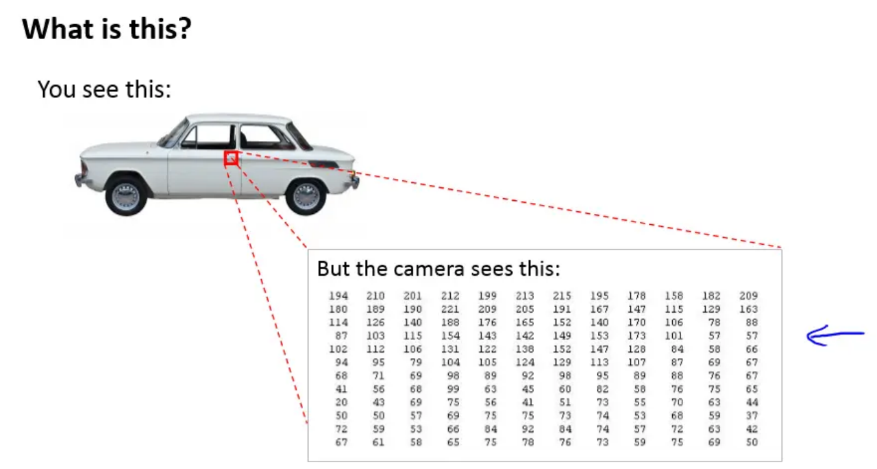
Core Insight from Computer Vision
- Direct approach from Computer Vision (CV) to GW signal processing: pixel point \(\Rightarrow\) sampling point.
- The CNN framework treats time series data similar to images, where each sampling point represents a feature to learn.
Performance Analysis
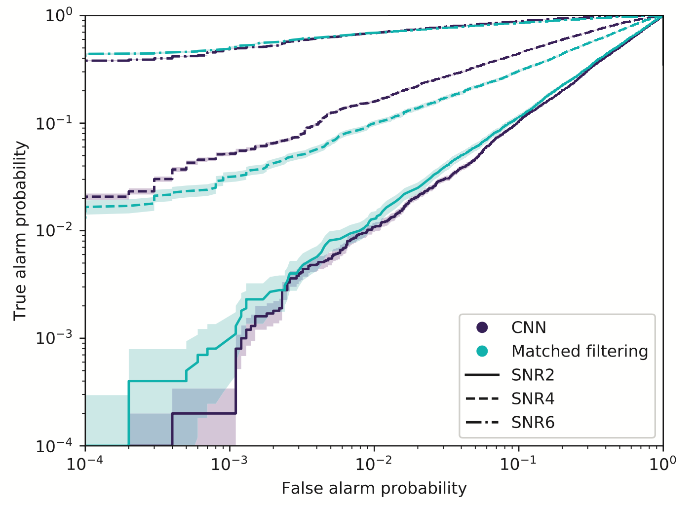
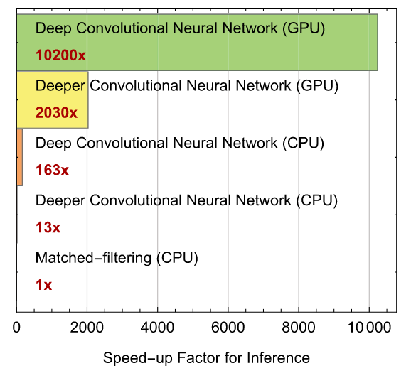
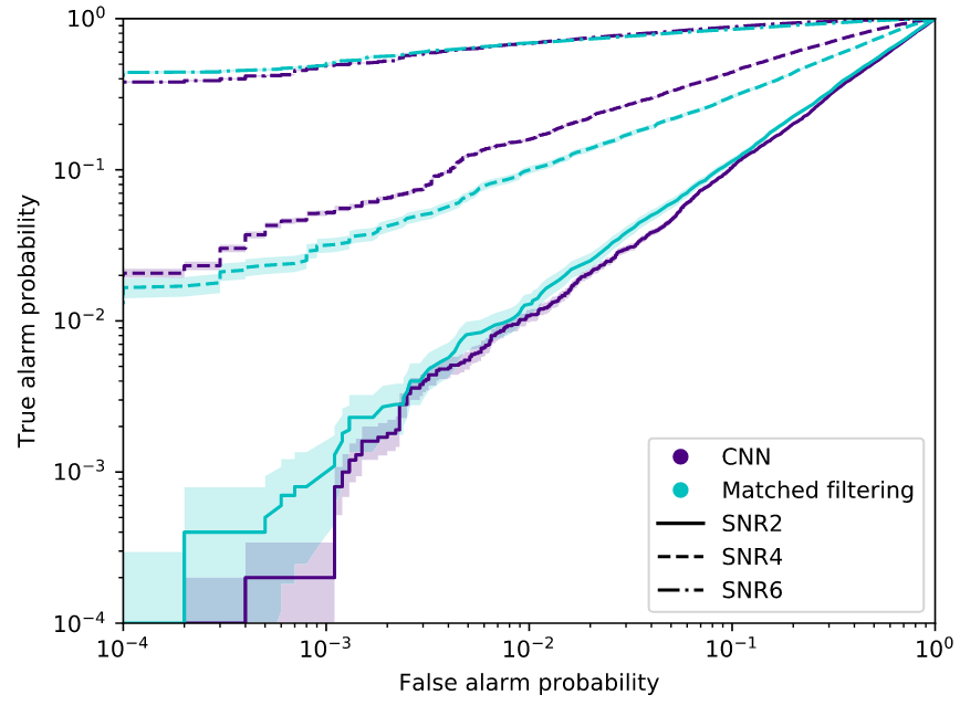
- Convolutional neural networks (CNN) can achieve comparable performance to Matched Filtering under Gaussian stationary noise.
- CNNs significantly outperform traditional methods in terms of execution speed (with GPU support).
- Modern architectures show improved robustness against non-Gaussian noise transients (glitches).
Pioneering Research Publications
PRL, 2018, 120(14): 141103.
PRD, 2018, 97(4): 044039.
# GW
CNN for GW Detection: Pioneering Approaches
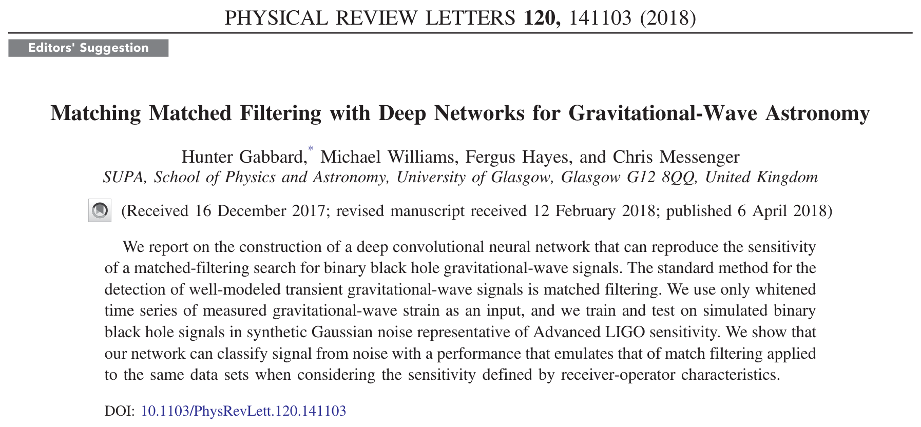
- Deep convolutional neural network to search for binary black hole gravitational-wave signals.
- Input is the whitened time series of measured gravitational- wave strain in Gaussian noise.
- Sensitivity comparable to match filtering.
A hands-on look at applying ML in real GW searches:
https://github.com/iphysresearch/GWData-Bootcamp
=> 2023/deep_learning/baseline/baseline_2025FQCP.ipynb
CNN Feature Extraction: Bridging Matched Filtering & Deep Learning
- Interpreting matched-filtering templates as predefined convolutional kernels within a neural network.
# GW: CNN

# GW
Convolution Neural Network (CNN)
Convolutional Neural Network (ConvNet or CNN)
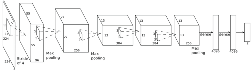
feature extraction
classifier
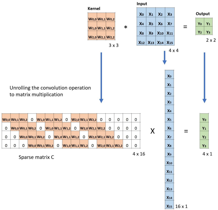
- Traditional Neural Networks vs Convolutional Neural Networks
- Convolutional layers are a special case of fully connected layers
- Fully connected layer:
- too many parameters, prone to overfitting
- Convolutional layer:
- Sparse Connectivity (sparse connectivity)
- Parameter Sharing (parameter sharing)
- Fully connected layer:
- Convolutional layers are a special case of fully connected layers
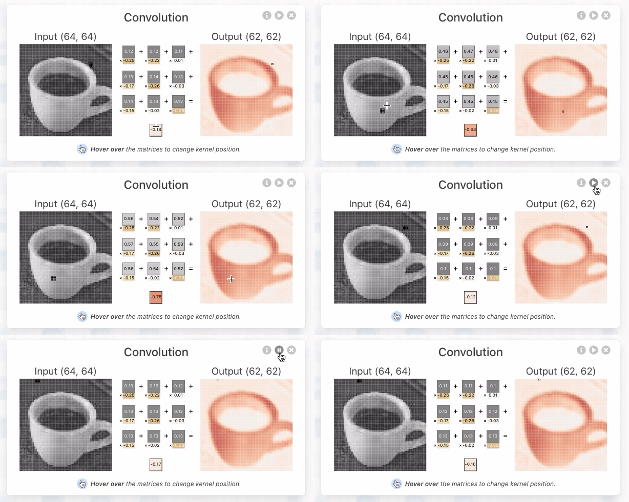
CNN Explainer:https://poloclub.github.io/cnn-explainer/
# GW
CNN for GW Detection: Feature Extraction
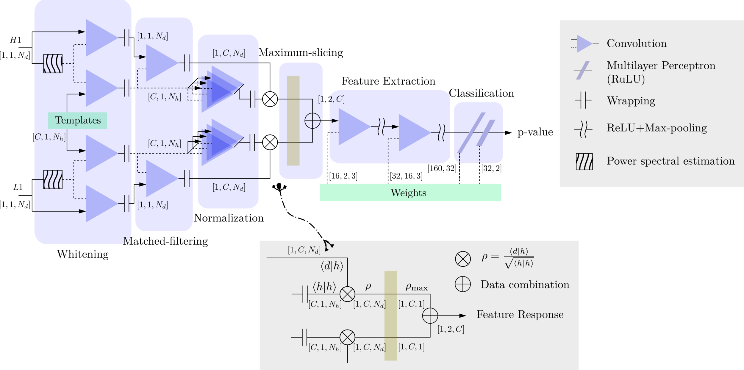
Matched-filtering Convolutional Neural Network (MFCNN)
HW, SC Wu, ZJ CAO, et al. PRD 101, 10 (2020): 104003
Convolutional Neural Network (ConvNet or CNN)
feature extraction
classifier
>> Is it matched-filtering ?
>> Wait, It can be matched-filtering!
- Matched-filtering (cross-correlation with templates) can be interpreted as a convolutional layer with predefined kernels.
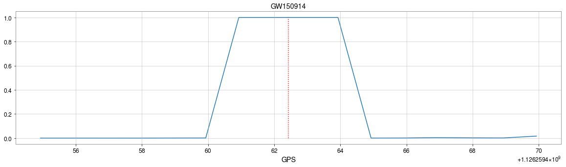
GW150914

GW150914
# GW
CNN for GW Detection: Feature Extraction
-
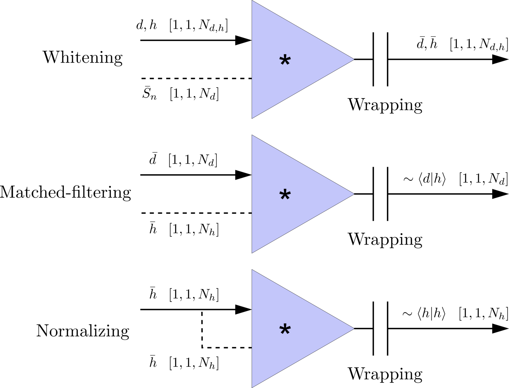
Transform matched-filtering method from frequency domain to time domain.
-
The square of matched-filtering SNR for a given data \(d(t) = n(t)+h(t)\):
\(S_n(|f|)\) is the one-sided average PSD of \(d(t)\)
where
Deep Learning Framework
Time Domain
(matched-filtering)
(normalizing)
(whitening)
Frequency Domain
# GW
CNN for GW Detection: Feature Extraction
-
Transform matched-filtering method from frequency domain to time domain.
-
The square of matched-filtering SNR for a given data \(d(t) = n(t)+h(t)\):
\(S_n(|f|)\) is the one-sided average PSD of \(d(t)\)
where
Deep Learning Framework
Time Domain
(matched-filtering)
(normalizing)
(whitening)
Frequency Domain
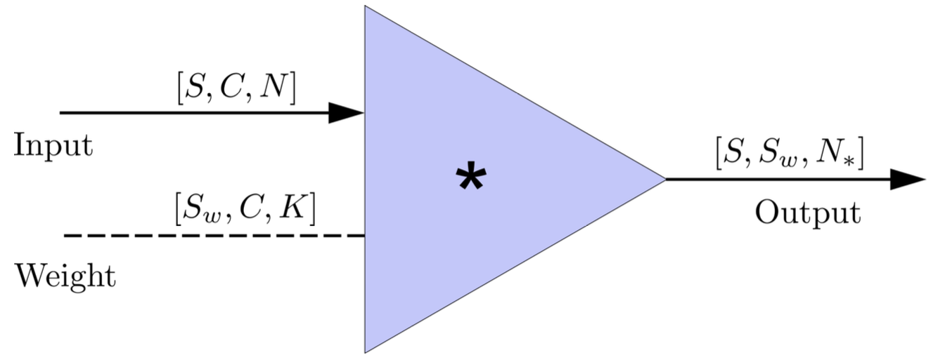
- In the 1-D convolution (\(*\)) on Apache MXNet, given input data with shape [batch size, channel, length] :
FYI: \(N_\ast = \lfloor(N-K+2P)/S\rfloor+1\)
(A schematic illustration for a unit of convolution layer)
# GW
CNN for GW Detection: Feature Extraction
import mxnet as mx
from mxnet import nd, gluon
from loguru import logger

def MFCNN(fs, T, C, ctx, template_block, margin, learning_rate=0.003):
    logger.success('Loading MFCNN network!')
    net = gluon.nn.Sequential()
    with net.name_scope():
        net.add(MatchedFilteringLayer(mod=fs*T, fs=fs,
                                      template_H1=template_block[:,:1],
                                      template_L1=template_block[:,-1:]))
        net.add(CutHybridLayer(margin = margin))
        net.add(Conv2D(channels=16, kernel_size=(1, 3), activation='relu'))
        net.add(MaxPool2D(pool_size=(1, 4), strides=2))
        net.add(Conv2D(channels=32, kernel_size=(1, 3), activation='relu'))
        net.add(MaxPool2D(pool_size=(1, 4), strides=2))
        net.add(Flatten())
        net.add(Dense(32))
        net.add(Activation('relu'))
        net.add(Dense(2))
	# Initialize parameters of all layers
    net.initialize(mx.init.Xavier(magnitude=2.24), ctx=ctx, force_reinit=True)
    return net
1 sec duration
35 templates used
Explainable AI Approach
- Implements matched filtering operations through custom convolutional layers
- Makes the network more interpretable by embedding domain knowledge
- Connects traditional signal processing with deep learning
- Outperforms standard CNNs in both accuracy and efficiency
Matched-filtering Convolutional Neural Network (MFCNN)
The available codes (2019): https://gist.github.com/iphysresearch/a00009c1eede565090dbd29b18ae982c
HW, SC Wu, ZJ CAO, et al. PRD 101, 10 (2020): 104003
# GW
First Benchmark for GW Detection Algorithms
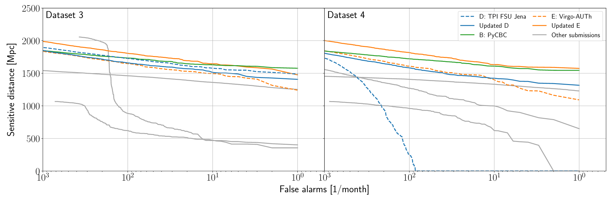
- Gravitational wave signal search algorithm benchmark (MLGWSC-1)
- Dataset-4: Sampled from O3a real gravitational wave observation data
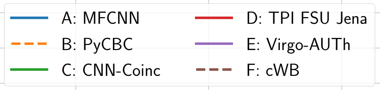

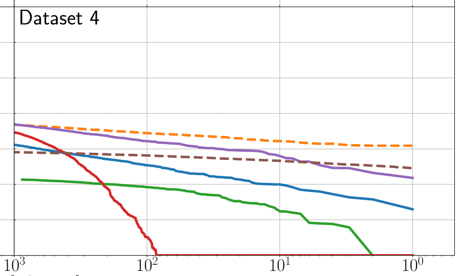


Benchmark Results
Publications
Key Findings
- On simulated noise data, machine learning algorithms are highly competitive compared to LIGO's most sensitive signal search pipelines
- Most tested machine learning algorithms are overly sensitive to non-Gaussian real noise backgrounds, resulting in high false alarm rates
- Traditional signal search algorithms can identify gravitational wave signals at low false alarm rates with assured confidence
- Tested machine learning algorithms have very limited ability to identify long-duration signals
Note on Benchmark Limitations:
Outperforming PyCBC doesn't conclusively prove that matched filtering is inferior to AI methods. This is both because the dataset represents a specific distribution and because PyCBC settings could be further optimized for this particular benchmark.
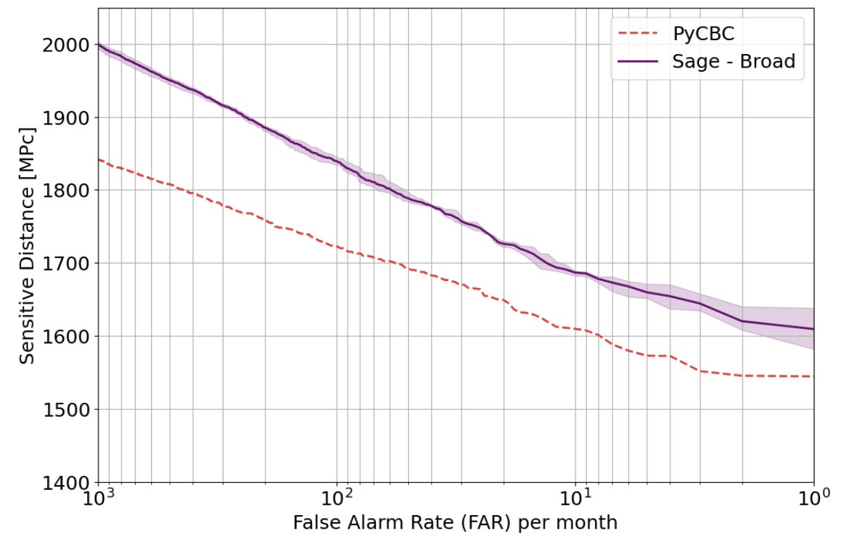
arXiv:2501.13846 [gr-qc]
Phys. Rev. D 107, 023021 (2023)
# GW
Interpretability Challenges:
Comparing Detection Statistics

-
Challenges in Model Interpretability:
- The black-box nature of AI models complicates interpretability, challenging the comparison of AI-generated detection statistics with traditional matched filtering chi-square distributions.
- Convincing the scientific community of the pipeline's validity and the statistical significance of new discoveries remains difficult despite the model's ability to identify potential gravitational wave signals.
AI Model Denoising
Our Model's Detection Statistics
LVK Official Detection Statistics
Signal denoising visualization using our deep learning model (Transformer-based)
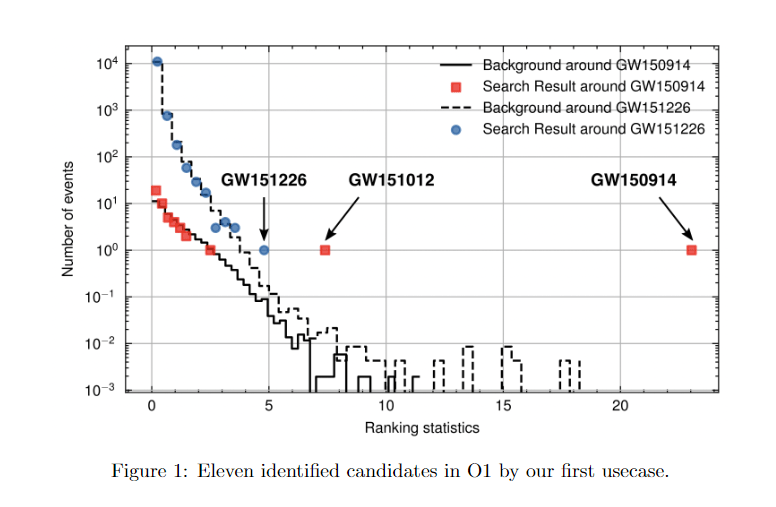
Detection statistics from our AI model showing O1 events
HW et al 2024 MLST 5 015046
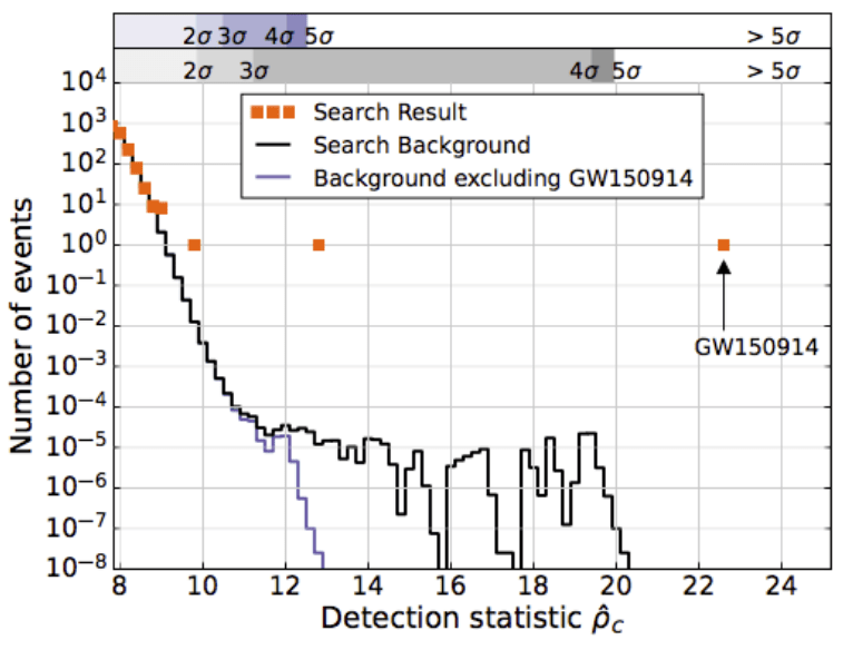
GW151226
GW151012
Official detection statistics from LVK collaboration
LVK. PRD (2016). arXiv:1602.03839

Content
-
What Is Machine Learning?
— The basics and why it matters -
Deep Learning: When Machines Start to See and Think
— From neural networks to powerful representations -
Gravitational Waves Meet Machine Learning
— How ML is reshaping data analysis in GW astronomy -
Natural Language Processing
— From transformer to three model families -
From Large Language Models to AI Agents
— Why are LLMs so powerful for automated scientific reasoning? -
Can AI Really Discover?
— From interpolation to search, verification, and science -
Harness Engineering for AI Agents
— How to utilize Claude Code, Codex, ...
Before LLMs: What was NLP?
Natural Language Processing (NLP) = teaching computers to work with human language
# NLP
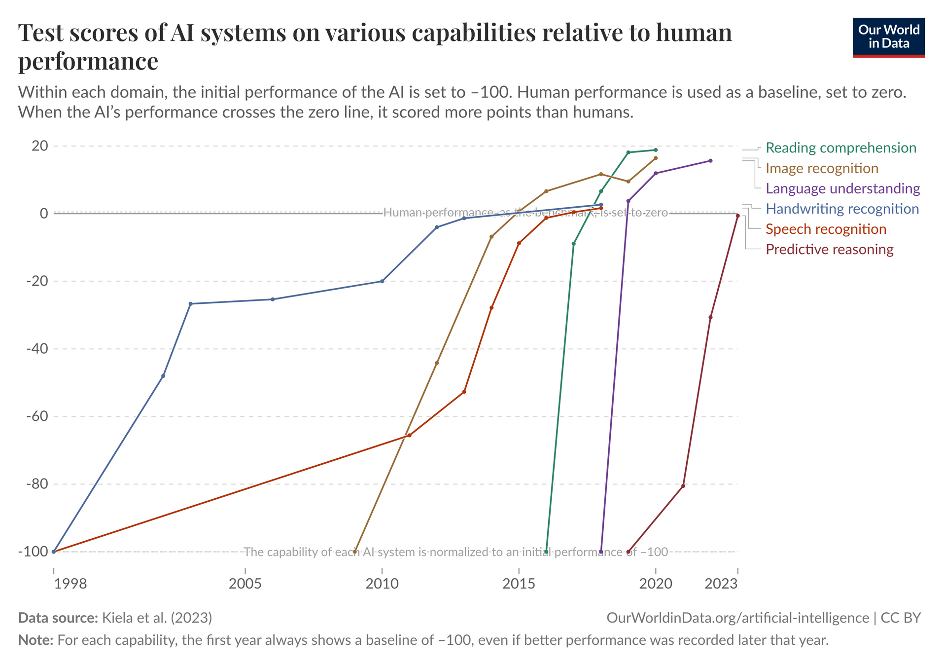
Human language → something computers can recognize, understand, predict, and generate
- translation · sentiment · QA · summarization · speech · search · …
Before LLMs: one task, one model.
- Different tasks had different datasets, architectures, objectives, and pipelines.
AI capabilities were improving — but separately.
Before LLMs: one task, one model.
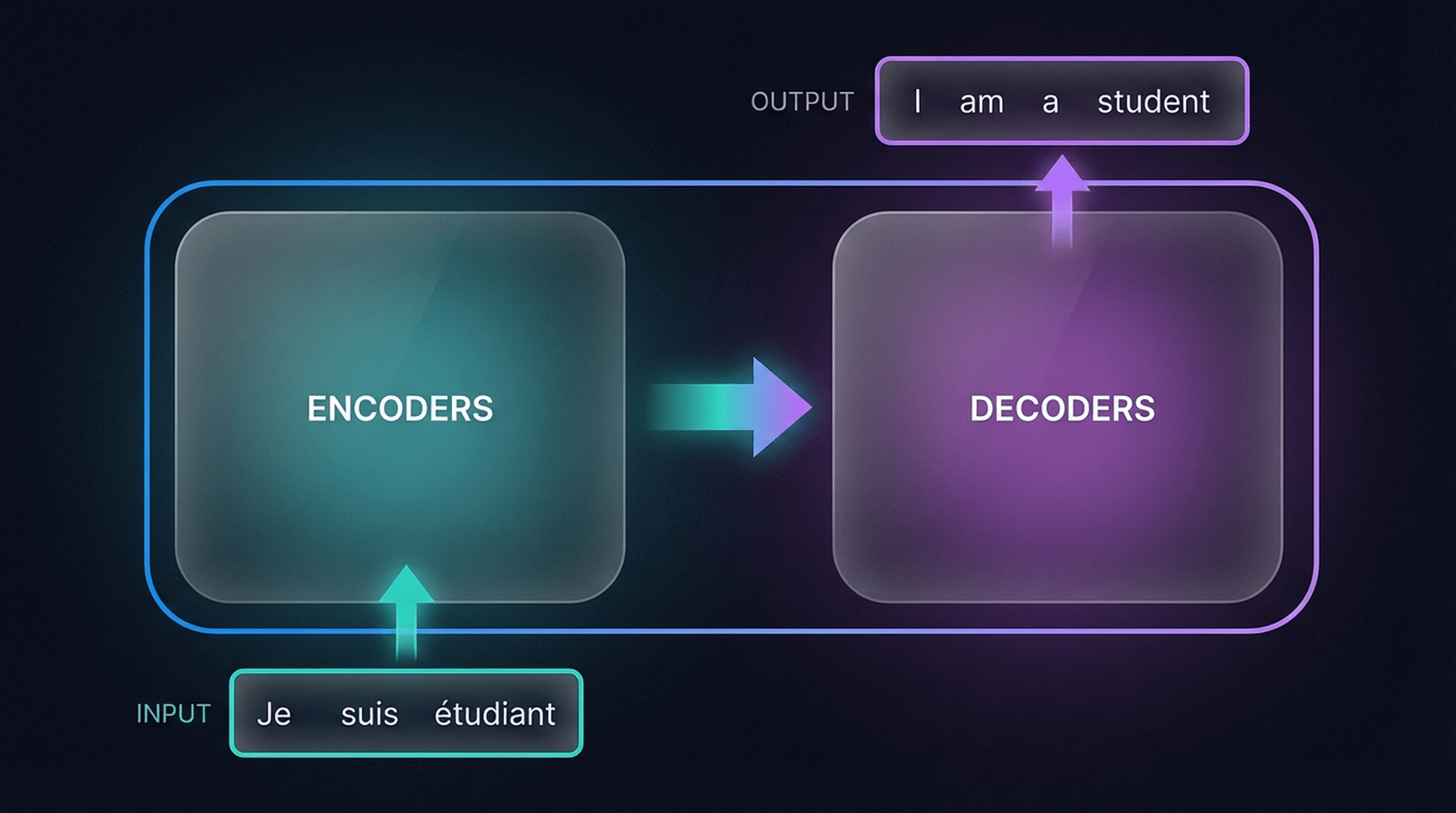
2017: The Transformer Changed NLP
“Attention Is All You Need” — from recurrent processing to attention-based sequence modeling
# NLP
The original Transformer was built for machine translation, not for ChatGPT.
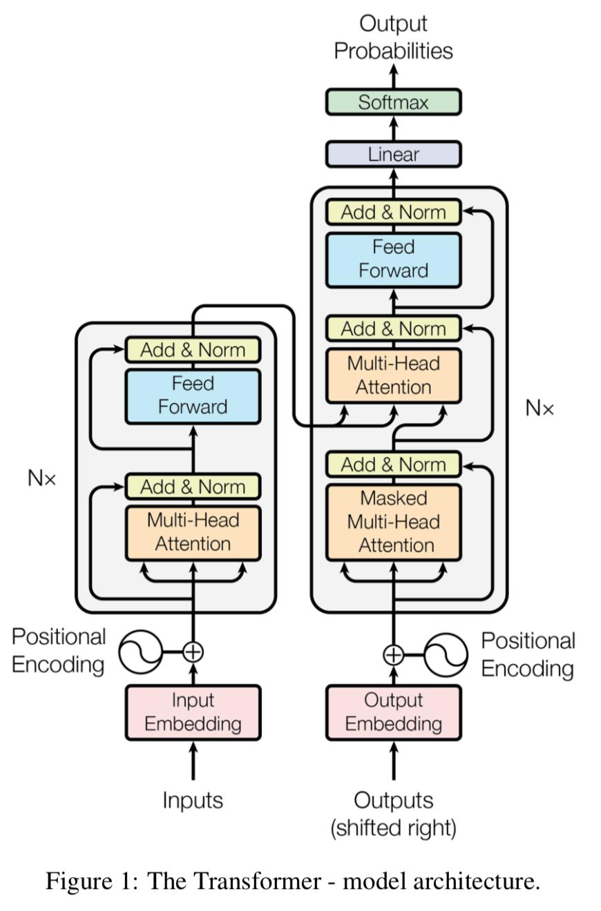
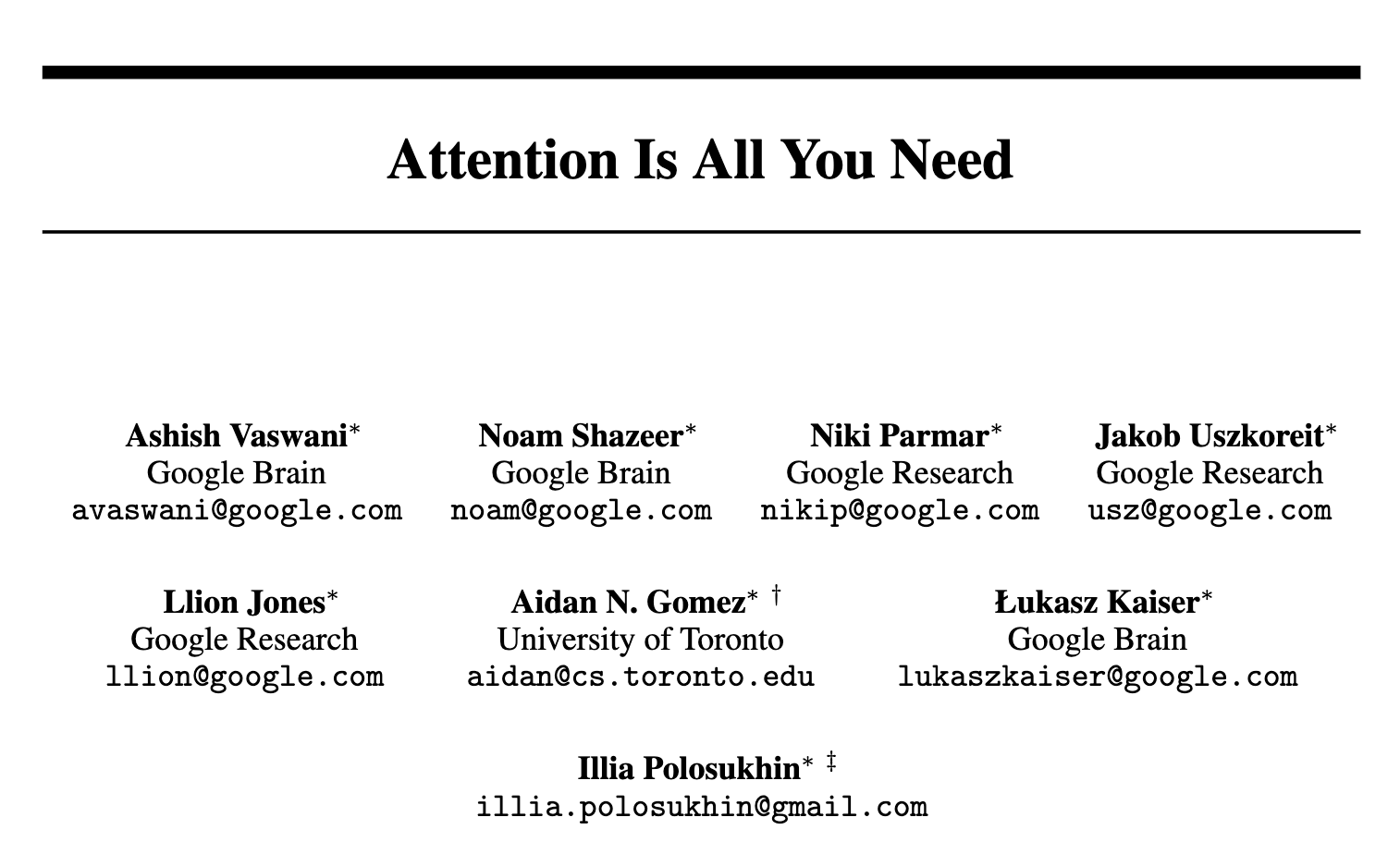
A paper for machine translation became the foundation of modern LLMs.
This architecture will be our map for the next few slides.
arXiv:1706.03762 [cs.CL]
Transformer Fundamentals: From Attention to Architecture
- Attention & Intuition: Query, Key, Value
- Parametric & Nonparametric Attention Pooling
- Attention Scoring Functions & Scaled Dot-Product
- Multi-Head Attention & Self-Attention
- Positional Encoding & Order Representation
- Feed-Forward Layers & Add & Norm Operations
# GW: NLP

Vanilla Transformer
Attention: “What should I look at?”
# NLP
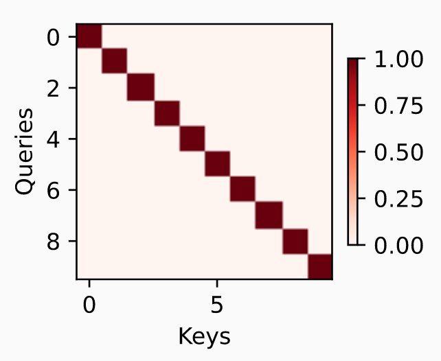
Given a query, attention measures its relevance to all keys, then uses these scores to combine the corresponding values.
Query
- What am I looking for?
Key
- What does each item contain / represent?
Value
- What information can I retrieve from it?
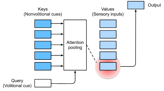
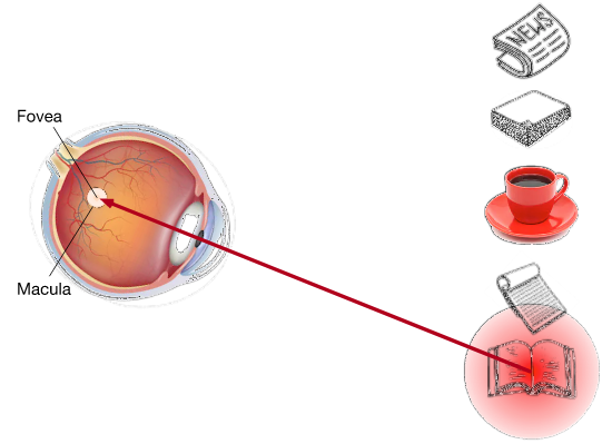
We do not process everything equally.
We focus on what is relevant.
Human intuition
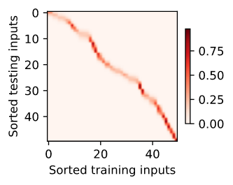
Attention Heatmap
(Color = attention weight)
Vanilla Transformer
Attention = Learn How Much Each Example Matters
# NLP
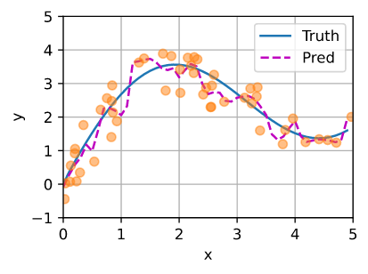
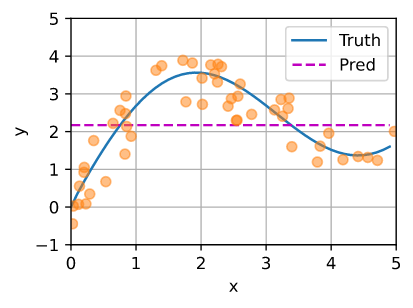
Consider a simple regression problem:
- given training pairs \(\{(x_i,y_i)\}_{i=1}^n\), how should we predict y for a new query x?
The key question is: should every training point contribute equally?
Case 1: Average Pooling
Case 2: Nonparametric Attention Pooling
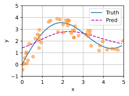
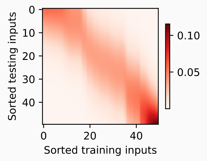
Case 3: Parametric Attention Pooling
Everyone matters equally
Ignores the query x.
Data:
\(\omega\) controls how selective the attention is — and it can be learned from data.
Vanilla Transformer
Attention Scoring Functions
# NLP
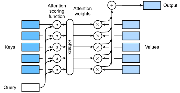
Query–Key similarity determines how much Value information is retrieved.
Given a query q and a set of key–value pairs \((k_i,v_i)\),
- scoring function \(a(q,k_i)\) measures the matching degree between the query and each key.
- Softmax converts scores into attention weights (\(\alpha_i\ge0,\ \sum_i\alpha_i=1\)):
- The output is the weighted sum of the values:
Transformer chooses a simple scoring function: dot product
queries \(Q \in \mathbb{R}^{n \times d}\), keys \(K \in \mathbb{R}^{m \times d}\) and values \(V \in \mathbb{R}^{m \times v}\) :
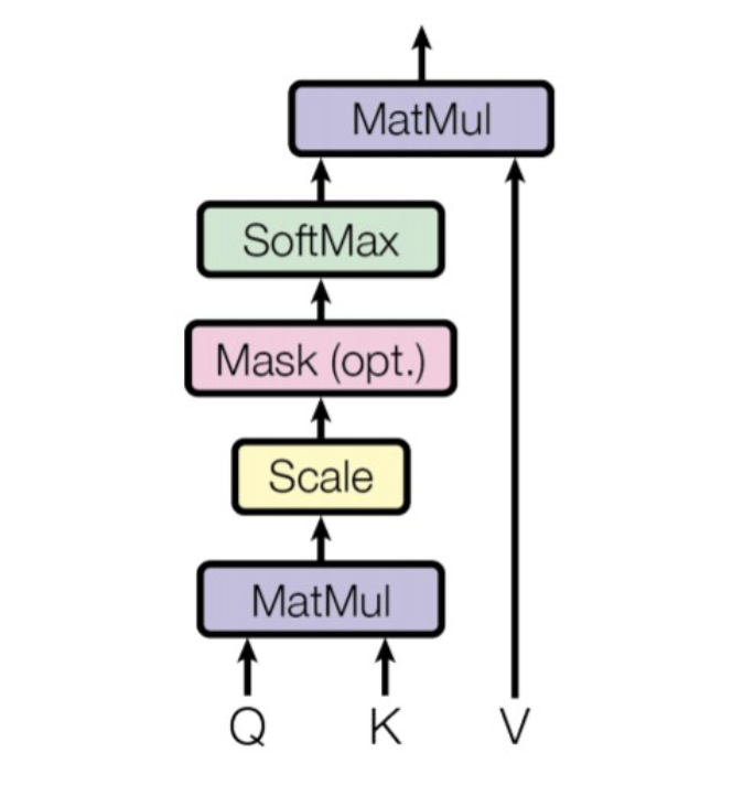
Q/K/V ~ [batch_size,len_tokens,dim_features]
[b, 15, 10]
[b, 15, 13]
[b, 15, 11]
[b, 13, 10]
[b, 13, 11]
In high dimensions, dot products become large; scaling sqrt(d) keeps softmax from becoming too saturated.
Vanilla Transformer
Multi-Head Attention & Self-Attention
# NLP
A single attention only measures relevance in one representation space; Multi-Head Attention allows the model to observe the same set of tokens from multiple representation subspaces simultaneously.
① Project
② Attend independently
③ Concatenate + mix
Note: More heads ≠ simply more copies of the same attention. Each head has its own learned projections \(W_i^Q,W_i^K,W_i^V\).
Self-attention means Q, K, and V are all derived from the same input sequence X. Each token looks at other tokens in the same sequence.
[batch_size * num_heads,
len_tokens,
dim_features / num_heads]
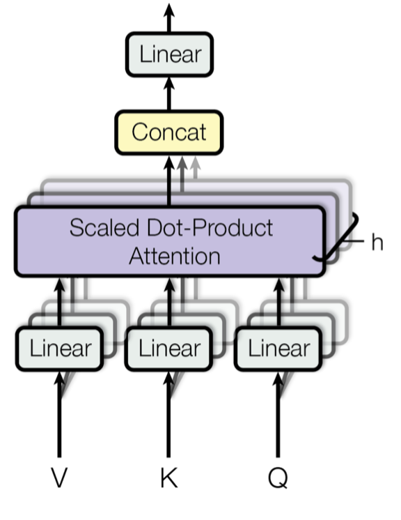
Q,K,V ~ [batch_size, len_tokens, dim_features]
[batch_size,
 len_tokens,
 dim_features]
[b, 5, 10]
[b, 5, 10]
[bx2, 5, 5]
(h=2)
Vanilla Transformer
Positional Encoding: Attention Has No Sense of Order
# NLP
Self-attention itself is permutation-insensitive: without extra position information, it does not know the order of tokens.
[batch_size, len_tokens]
[batch_size,
 len_tokens,
 dim_features]
[batch_size,
 len_tokens,
 dim_features]
Token embedding
“What is this token?”
Positional encoding
“Where is this token?”
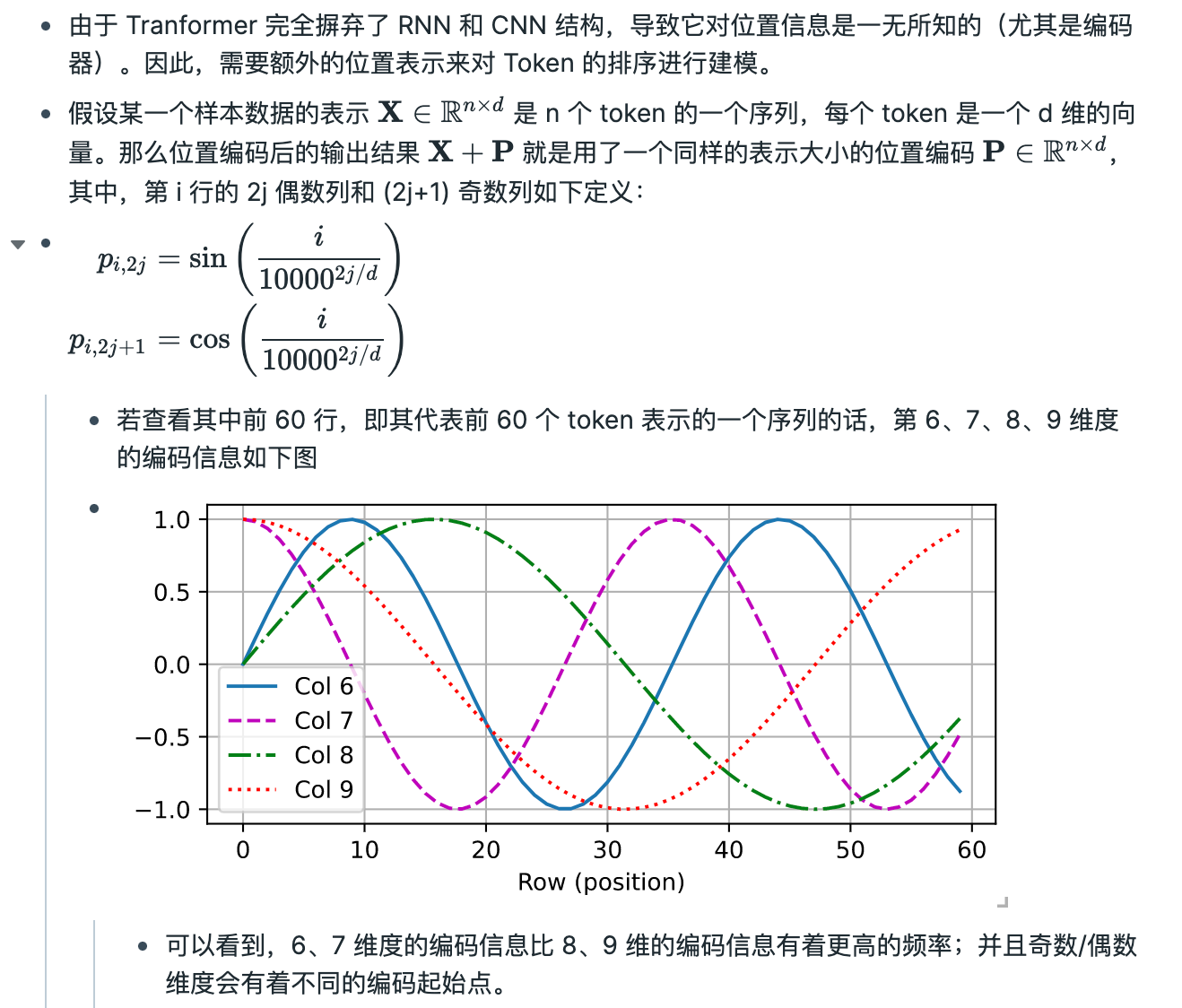
- Different dimensions encode position at different frequencies
- Even dimensions use sine, odd dimensions use cosine.
This means that the model can not only know "the position of the token", but also relatively easily learn "how far apart two tokens are" from the representation.
- Original Transformer (2017): sinusoidal positional encoding
-
Modern LLMs often use other schemes, e.g. learned embeddings or RoPE.
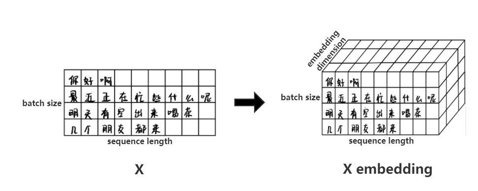
Since the Transformer completely abandons RNN and CNN structures, it is completely unaware of positional information (especially the encoder). Therefore, additional positional representations are needed to model the ordering of Tokens.
Assuming a representation of a sample data \(\mathbf{X} \in \mathbb{R}^{n \times d}\) is a sequence of n tokens, where each token is a d-dimensional vector. Then the output result after position encoding \(\mathbf{X}+\mathbf{P}\) uses a position encoding \(\mathbf{P} \in \mathbb{R}^{n \times d}\) of the same representation size, where the 2j even-indexed columns and the \((2 \mathrm{j}+1)\) odd-indexed columns of the i-th row are defined as follows:
It can be seen that the encoding information of dimensions 6 and 7 has a higher frequency than that of dimensions 8 and 9; and the odd/even dimensions will have different encoding starting points.
If you look at the first 60 rows, which represent a sequence of the first 60 token representations, the encoding information for dimensions 6, 7, 8, and 9 is shown in the figure below.
Vanilla Transformer
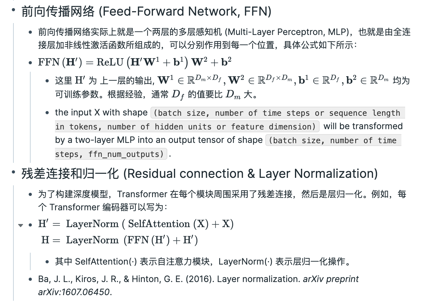
Feed-Forward + Add & Norm
# NLP
Attention mixes tokens; FFN transforms each token.
[batch_size,
 len_tokens,
 dim_features]
[batch_size,
 len_tokens,
 dim_features]
[batch_size, len_tokens, dim_features]
K
V
Q
Vanilla Transformer
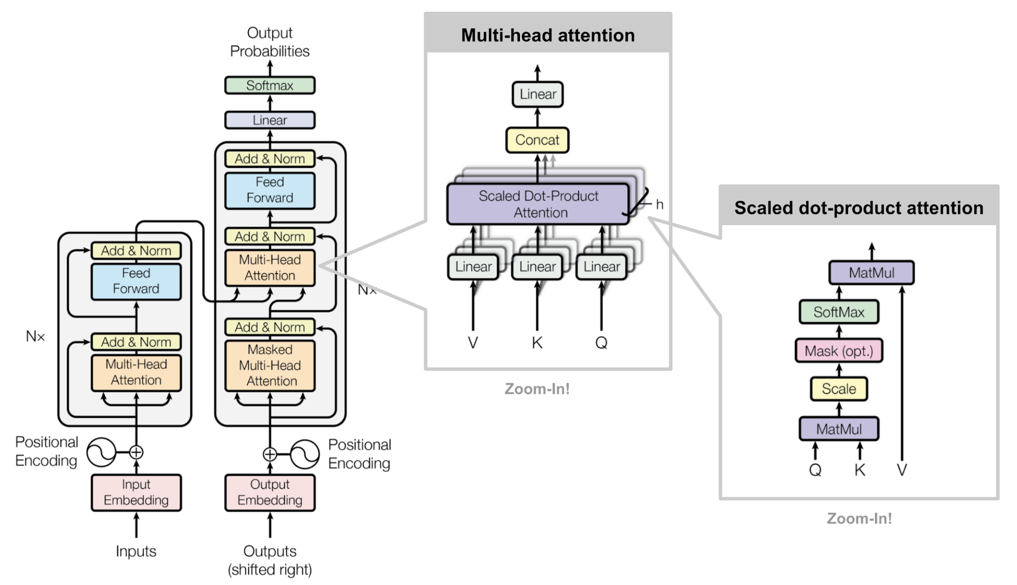
# NLP
Now we can read the whole Transformer from bottom to top.
Q from Decoder
K,V from Encoder
[batch_size,
 len_tokens1,
 dim_features1]
[batch_size, len_tokens2]
[batch_size, len_tokens2, vocal_size]
K
V
Q
[batch_size,
 len_tokens1,
 dim_features1]
[batch_size,
 len_tokens2,
 dim_features2]
[batch_size, len_tokens1]
, len_tokens1]
Vanilla Transformer
# NLP
[batch_size,
 len_tokens1,
 dim_features1]
[batch_size, len_tokens1]
[batch_siz
[batch_size, len_tokens2, vocal_size]
[batch_size,
 len_tokens1,
 dim_features1]
[batch_size,
 len_tokens2,
 dim_features2]
K
V
Q
Now we can read the whole Transformer from bottom to top.
[batch_size, len_tokens2]
, len_tokens1]
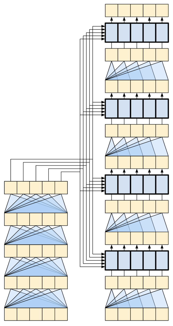
- Deep Stacked Architecture:
It shows the multi-layer stack implementation (\(\times\)) where features are refined through stacked Encoder layers and decoded through corresponding Decoder layers with residual connections.
Source: X
Vanilla Transformer
# NLP
Now we can read the whole Transformer from bottom to top.
Source: X
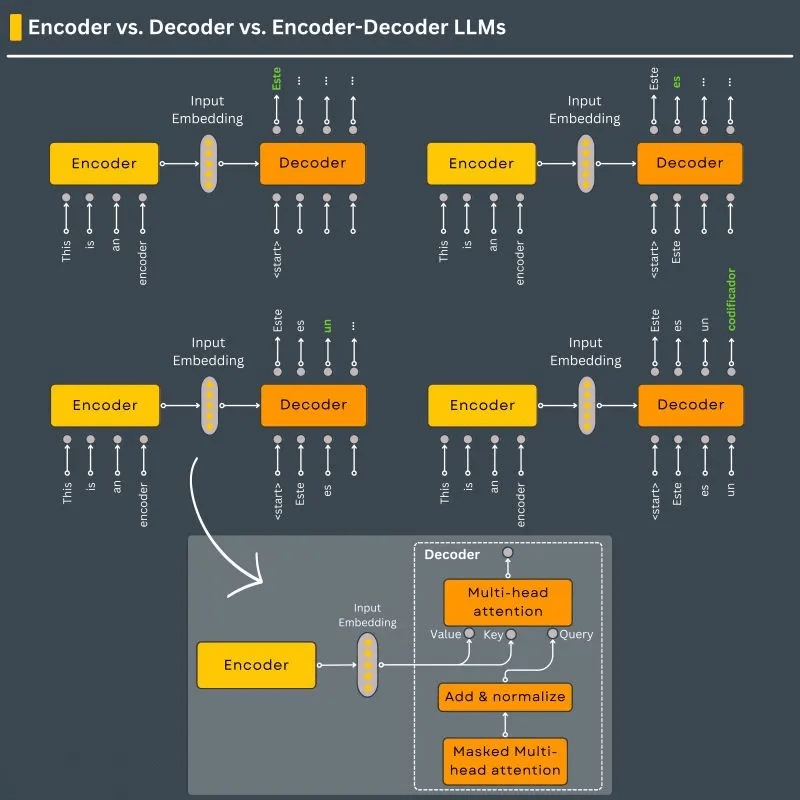
Source: X
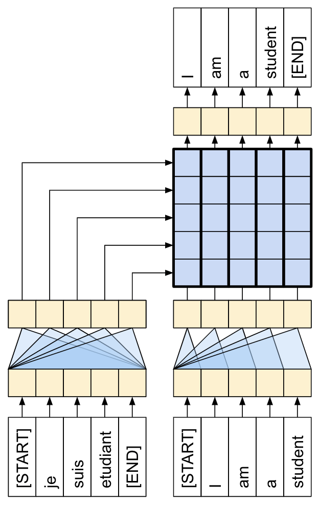
- Inference / Translation Flow:
It illustrates the autoregressive inference process where the Encoder encodes the source sentence once, and the Decoder iteratively predicts the next token step-by-step using cross-attention and previously generated tokens.
Source: X
Vanilla Transformer
# NLP
[batch_size, len_tokens2, vocal_size]
Source: X
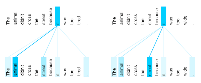
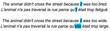
The encoder self-attention distribution for the word “it” from the 5th to the 6th layer of a Transformer trained on English to French translation (one of eight attention heads).
What Does Self-Attention Learn?
Same word, different context → different reference
Query: “it”
Keys: all words in the sentence
Attention weight: how strongly “it” attends to each word
One step to connect distant tokens — and we can visualize the connection.
The Three Model Families & The Rise of Generative LLMs
- From Transformer to Three Model Families
- Why Did Decoder-Only Win the LLM Race?),
# GW: NLP
WaveFormer
# NLP
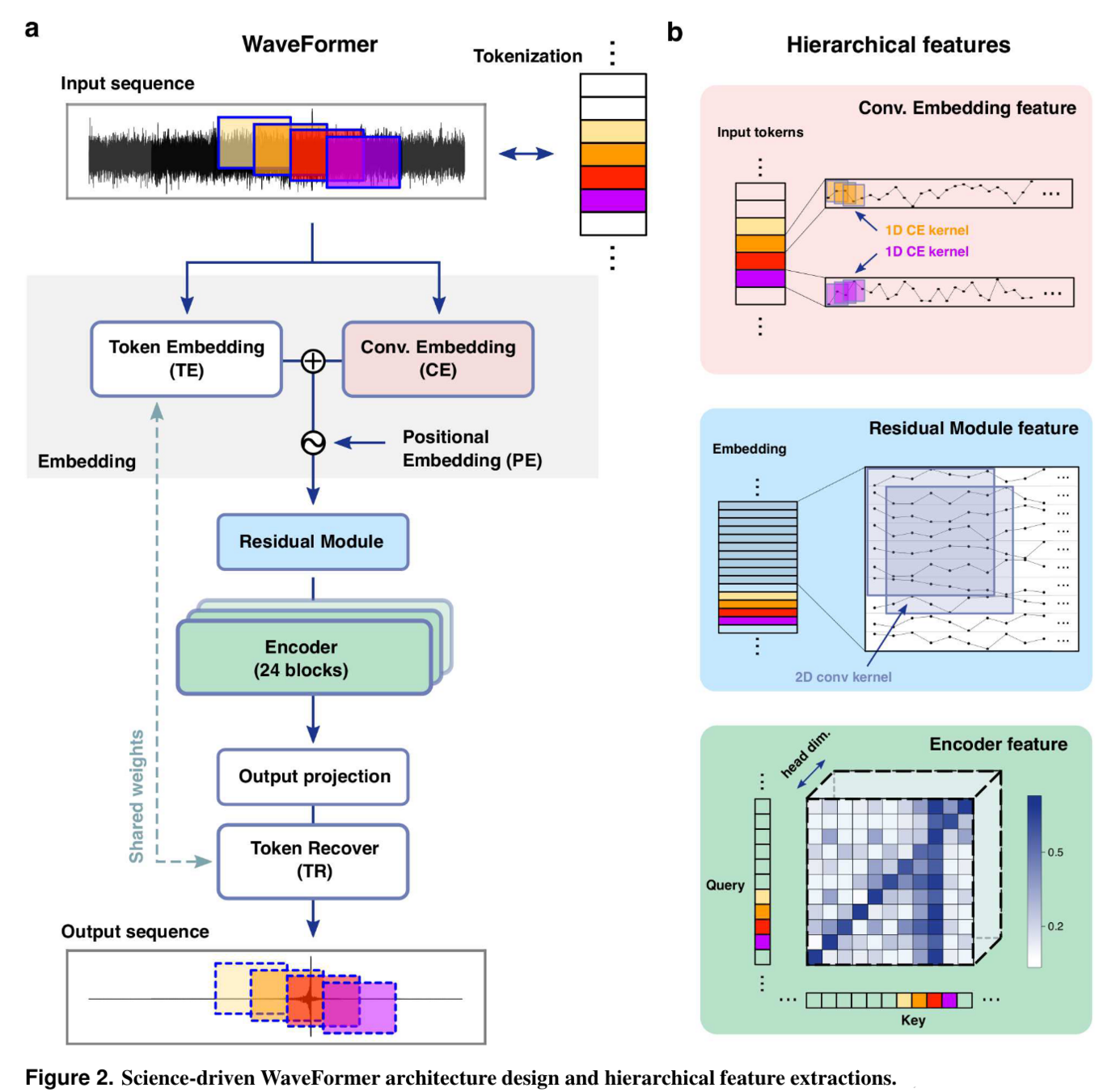



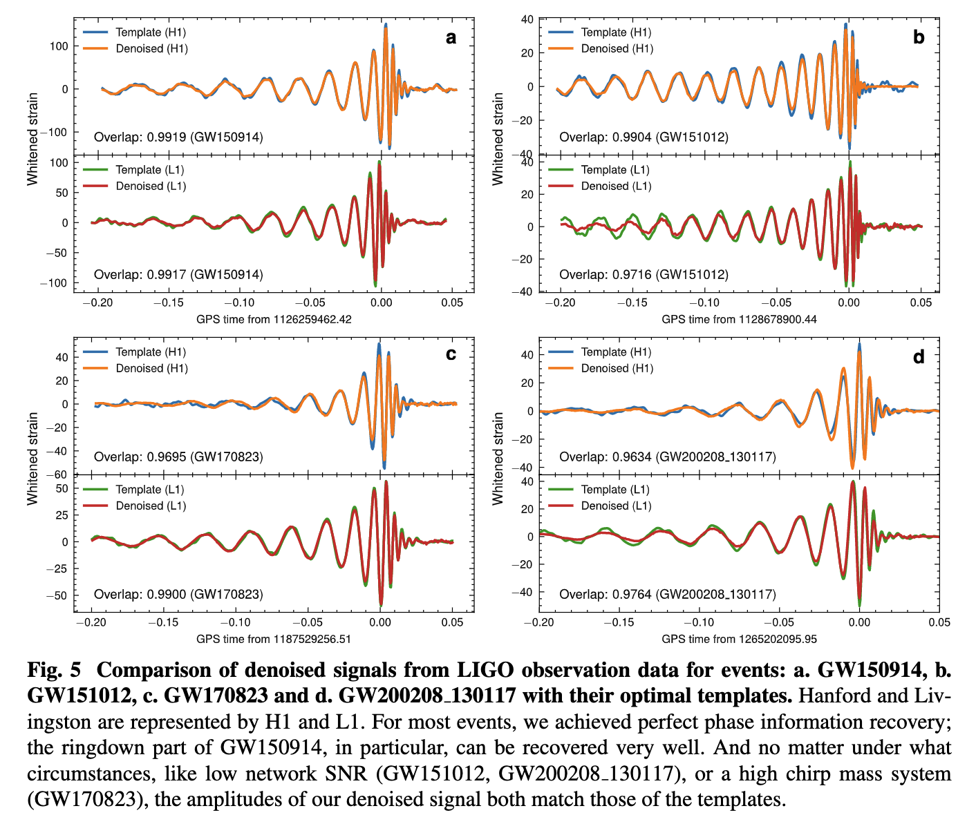
HW+ 2024 MLST 5 015046
Leveraging the Transformer Encoder for Gravitational-Wave Denoising & Representation
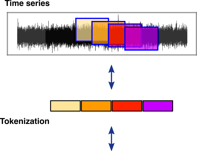
["This", "is", "a", "sample"]
[1, 16512]
[1, 128, 256]
From Transformer to Three Model Families
# NLP
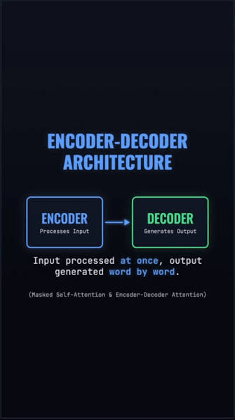
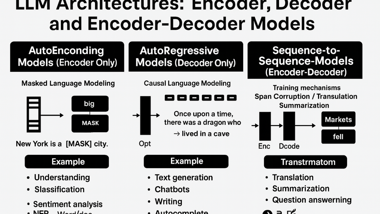
Encoder vs. Encoder–Decoder vs. Decoder
Source: X
① Encoder-only
Read everything
Typical tasks: classification · retrieval · NER · embeddings- Typical models: BERT · RoBERTa
② Encoder–Decoder
Read, then generate
- Typical tasks: translation · summarization · seq2seq
- Typical models: T5 · BART · original Transformer
③ Decoder-only
Predict what comes next
- Typical models: GPT family · LLaMA
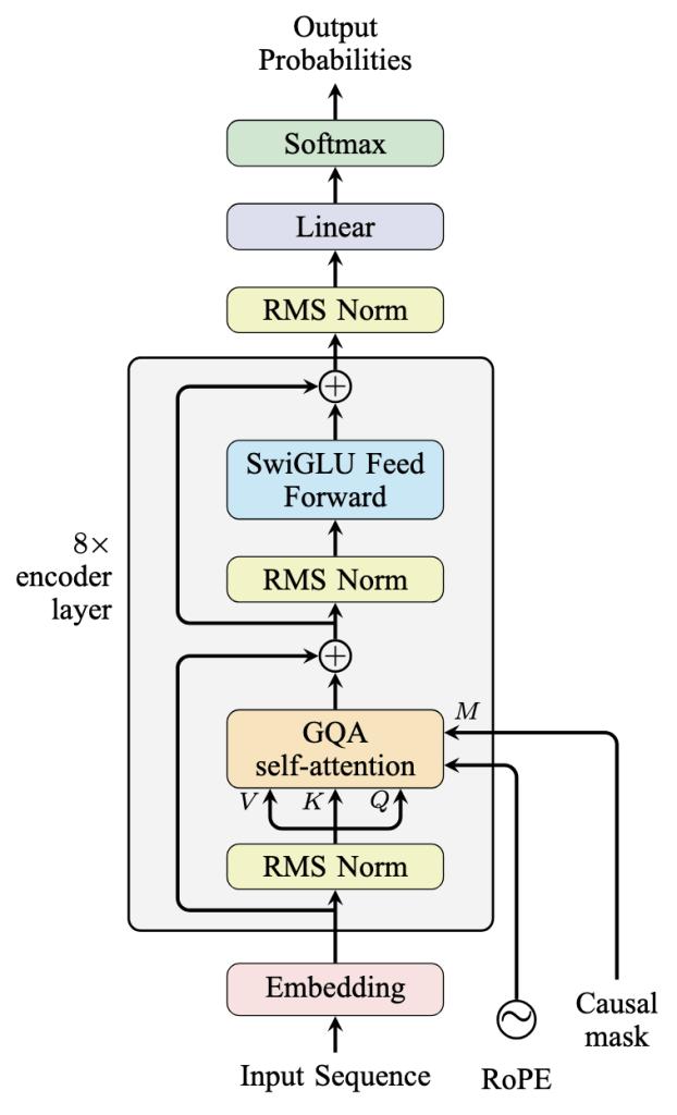
Eg:
Decoder-Only Model Following the Architecture of Llama-2/Llama-3
Source: X
Why Did Decoder-Only Win the LLM Race?
# NLP
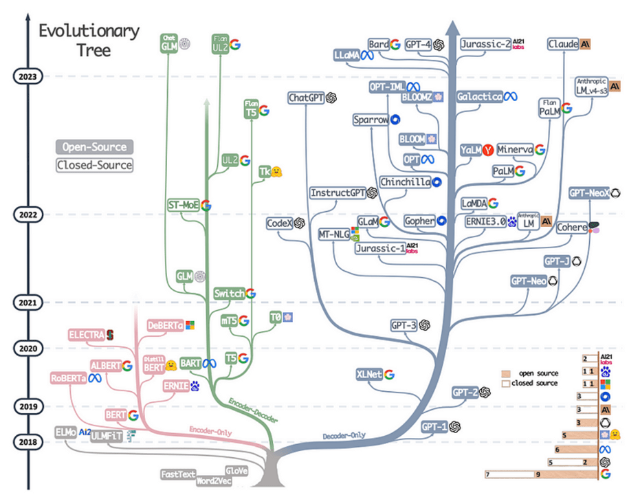
Three branches emerged — but one became dominant for general-purpose LLMs.
BERT vs GPT
Two self-supervised objectives, two very different futures
GPT
\(\text{The cat sat on the} \rightarrow ?\)
Predict next token.
Causal
Generation-oriented
BERT
\(\text{The cat [MASK] on the mat}\)
Predict masked token.
Bidirectional
Representation-oriented
Excellent representations / understanding
The path that scaled into general-purpose LLMs
2018–2019
BERT looked extremely powerful
2020+
GPT-style scaling changed the game
This figure stops around 2023.
Excellent sequence-to-sequence models

Content
-
What Is Machine Learning?
— The basics and why it matters -
Deep Learning: When Machines Start to See and Think
— From neural networks to powerful representations -
Gravitational Waves Meet Machine Learning
— How ML is reshaping data analysis in GW astronomy -
Natural Language Processing
— From transformer to three model families -
From Large Language Models to AI Agents
— Why are LLMs so powerful for automated scientific reasoning? -
Can AI Really Discover?
— From interpolation to search, verification, and science -
Harness Engineering for AI Agents
— How to utilize Claude Code, Codex, ...
GPT-3 → GPT-3.5: The “Code” Turning Point
# LLM
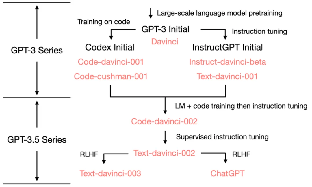
Training on code did more than teach the model programming.
Why training Python, JavaScript, GitHub code can actually enhance a language model's natural language reasoning?
-
Code forces the model to learn precise structure.
-
Code is full of explicit intermediate computation.
-
Small components must compose correctly into a working whole.
A code-trained model became the base of the GPT-3.5 lineage.
GPT-3 (2020)
ChatGPT (2022)
Magic: Code + Text
John has 3 apples and buys 2 more.
How many does he have?
apples = 3
apples += 2
print(apples)Natural language
Code
Same semantics — but code makes variables, operations, and state explicit.
# LLM
Training on code did more than teach the model programming.
Why training Python, JavaScript, GitHub code can actually enhance a language model's natural language reasoning?
-
Code forces the model to learn precise structure.
-
Code is full of explicit intermediate computation.
-
Small components must compose correctly into a working whole.
A code-trained model became the base of the GPT-3.5 lineage.
GPT-3 (2020)
ChatGPT (2022)
Magic: Code + Text
John has 3 apples and buys 2 more.
How many does he have?
apples = 3
apples += 2
print(apples)Natural language
Code
Same semantics — but code makes variables, operations, and state explicit.
Why Are LLMs So Powerful? — ① Code
Why Are LLMs So Powerful? — ② Scaling
More compute, more data, larger models → predictably lower loss
Why scaling matters
Predictable
- We can forecast larger-model performance.
Continuous
- Capability keeps improving over large resource ranges.
Composable
- Scaling later expanded beyond pretraining.
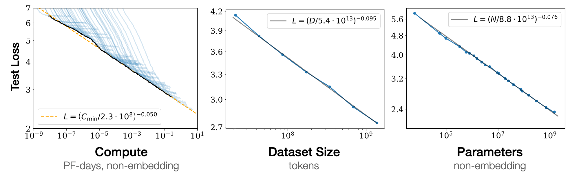
arXiv:2001.08361 [cs.LG]
Performance did not saturate as quickly as people expected.
# LLM
Why Are LLMs So Powerful? — ③ Programmability
From explicit rules to natural-language control
Rule-Based Vs. LLMs: (Source)
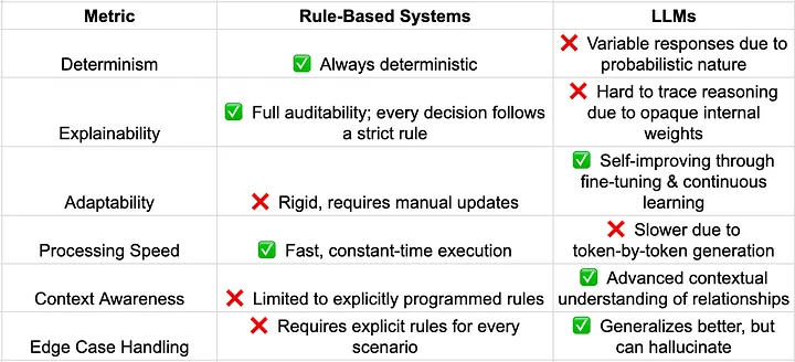
LLMs are not only models; they are becoming a programmable interface to software, data, and the physical world.
if sender in VIP_LIST \
   or "urgent" in subject \
   or "!" in subject \
   or priority == "high":
    notify()
❌ brittle rules
❌ unseen wording
❌ endless edge cases
Traditional Programming
Program the condition
LLM Programming
Describe the condition
if LLM(
  "Does this message require
   an important action soon?"
).parse():
    notify()
If I receive an email marked "important and requires my prompt attention," just remind me.
- “Could you send me the revised figure before tomorrow’s meeting?”
- “URGENT: Our summer sale ends tonight!”
✓ semantic
✓ context-aware
✓ adaptable to unseen cases
Code controls the flow;
language defines the condition.
# LLM
Why Are LLMs So Powerful? — ③ Programmability
From explicit rules to natural-language control
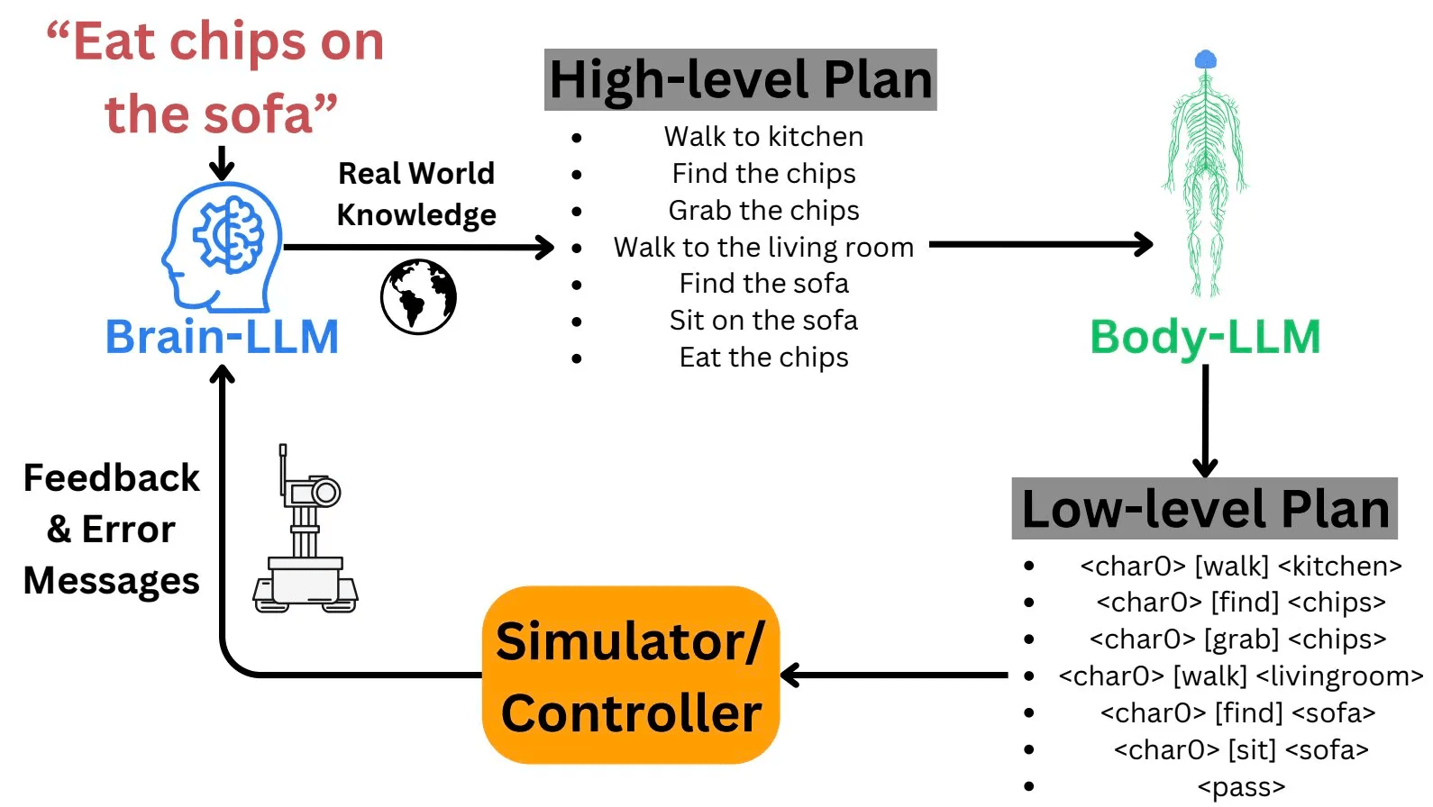
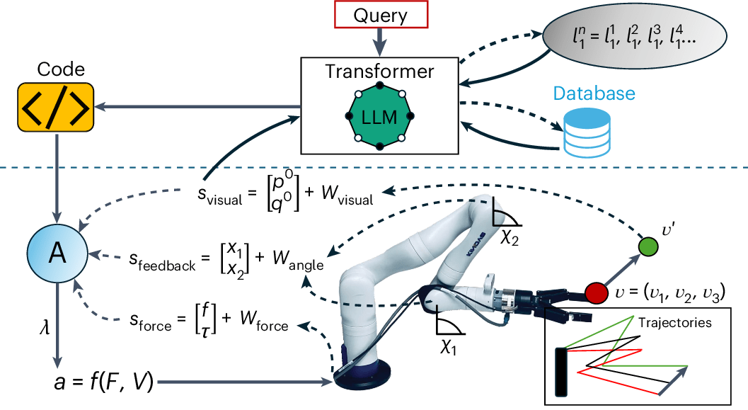
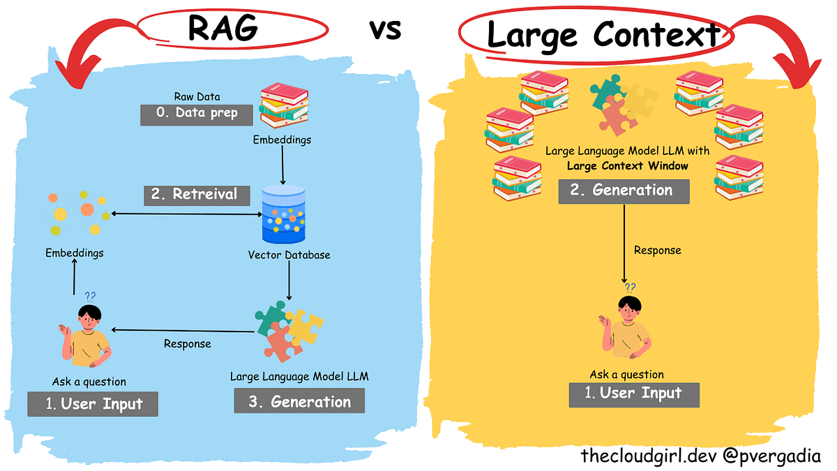
Rule-Based Vs. LLMs: (Source)
LLMs are not only models; they are becoming a programmable interface to software, data, and the physical world.
# LLM
Why Are LLMs So Powerful? — ③ Programmability
From explicit rules to natural-language control
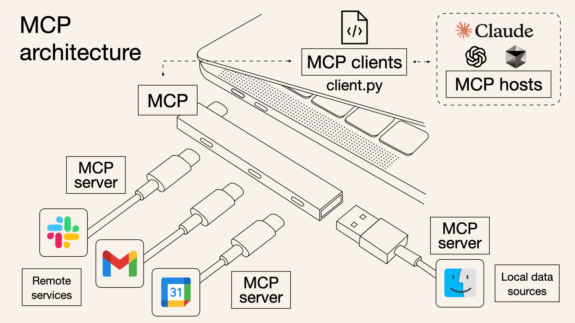
The Model Context Protocol (MCP) is an open-source protocol launched by Anthropic, aimed at achieving the integration of large language models with external data sources and tools, to establish a secure bi-directional connection between large models and data sources.
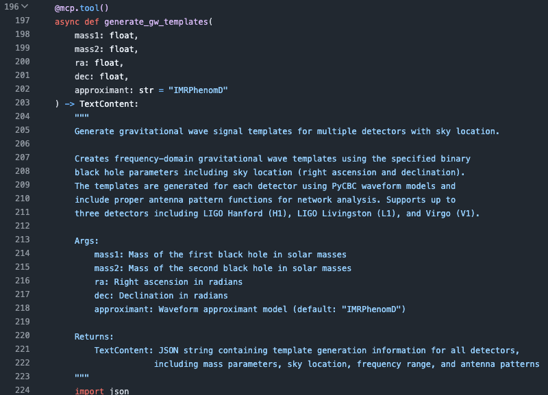
MCP Tool
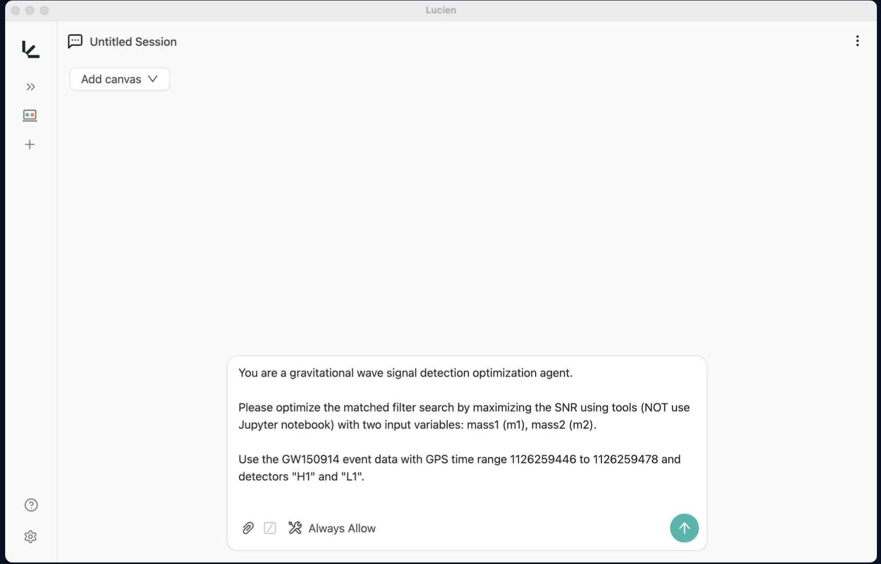
prompt
"Please generate gw templates first."Demo: GW150914 MCP Signal Search
# LLM
Why Are LLMs So Powerful? — ③ Programmability
From explicit rules to natural-language control
if chi_square > 10:
    rerun_analysis()
Traditional Programming
Program the condition
LLM Programming
Describe the condition
if LLM(
    """
    Given the diagnostic plots, residuals,
    logs, and previous runs:
    does this result show evidence of
    a meaningful model-data mismatch
    that warrants another analysis?
    """).parse():
    rerun_analysis()
Previously,
conditionhad to be a value criterion defined in advance by a programmer.
Now, condition can be a comprehensive judgment on text, images, logs, context, and even scientific semantics.
This is where LLMs start to become agents.
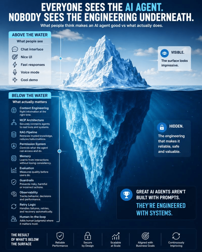
# LLM
Why Agents? Test-Time Scaling & Feedback Loops
- LLMs in the Loop: Moving from one-shot generation to iterative interaction (Generate → Observe → Act → Refine)
- The Evolution of Scaling: Pre-training $\rightarrow$ Post-training $\rightarrow$ Test-time compute & reasoning
- LLM Foundations: Pre-training, instruction tuning, alignment, and GRPO reasoning
- Generative Agents & Tool Use: Memory, planning, and execution in scientific environments
# GW: LLM

From LLMs to Scientific Discovery
# Agent
Generate → Observe → Act → Refine
One-shot generation → iterative interaction
An agent is not a new neural network. It is an LLM placed inside a loop.
Can't do it directly?
Then let's package it up and try again!
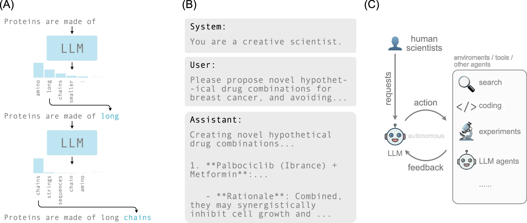
npj Artif. Intell. 1, 14 (2025).
"Sequence Output"
"Sequence Input"
"Direct fails. Refine and recover."
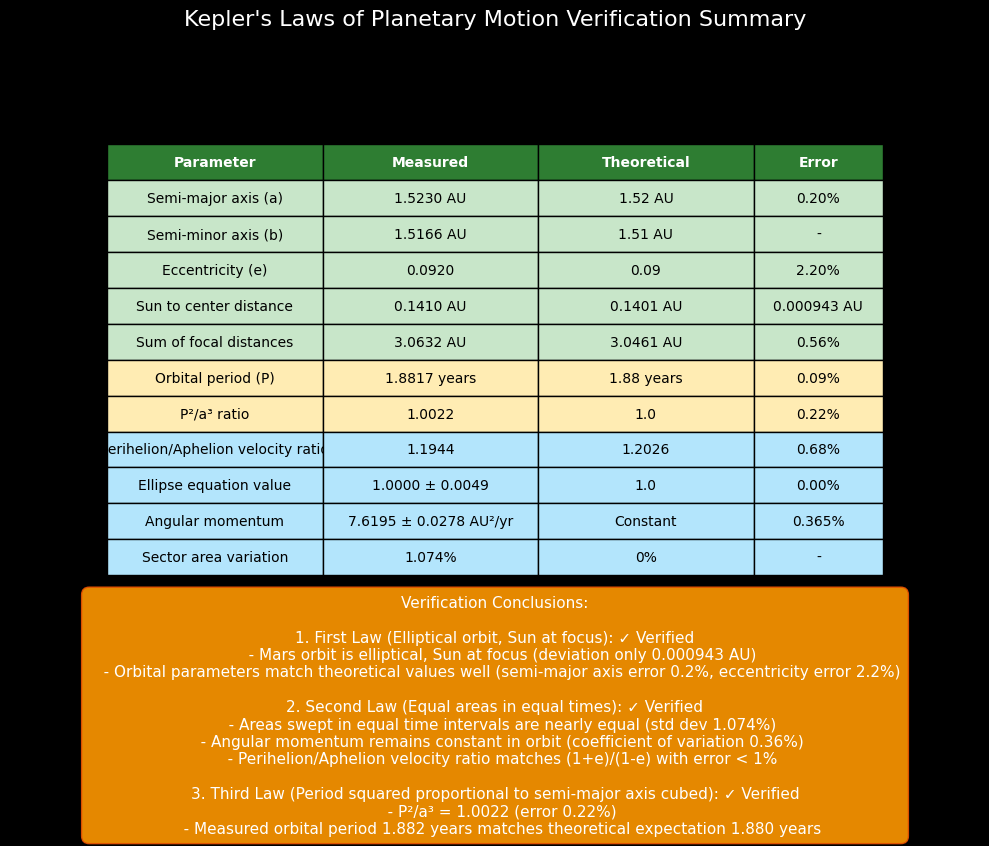
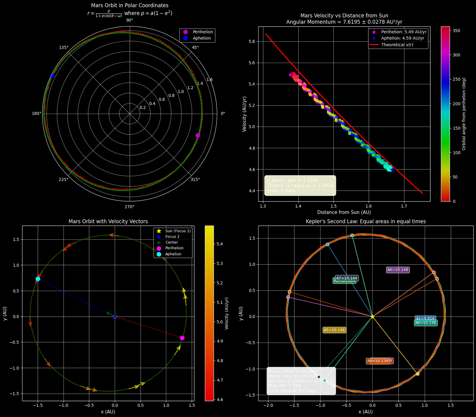
Demo (2025): LLM Validation of Kepler's Three Laws of Planetary Motion
From LLMs to Scientific Discovery
# Agent
Generate → Observe → Act → Refine
One-shot generation → iterative interaction
An agent is not a new neural network. It is an LLM placed inside a loop.
Can't do it directly?
Then let's package it up and try again!
npj Artif. Intell. 1, 14 (2025).
"Sequence Output"
"Sequence Input"
"Direct fails. Refine and recover."
Agent does not necessarily mean that we have invented an entirely new model.
Many times, it simply puts the LLM into an "observe-decide-act-feedback" loop.
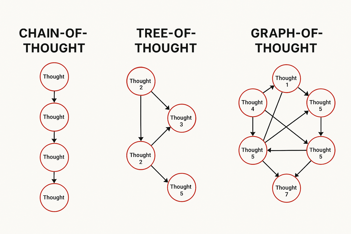
arXiv:2201.11903 [cs.CL]
arXiv:2305.10601 [cs.CL]
# Agent
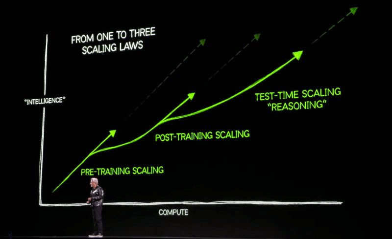
This is where test-time scaling begins to look like an agent.
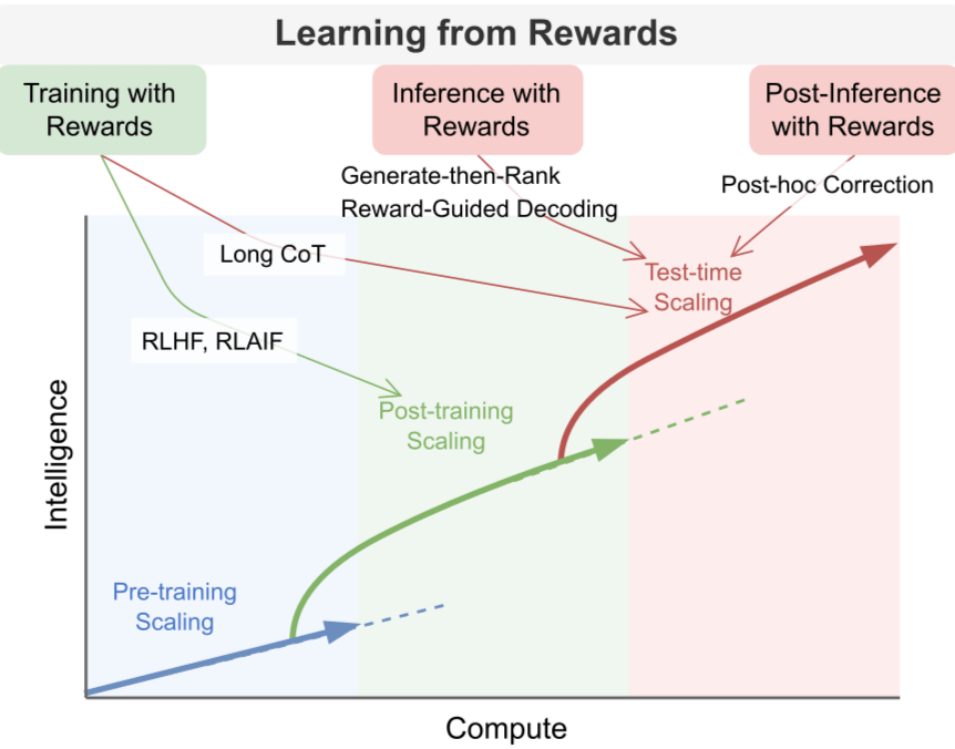
2020-era intuition
Pre-training scaling
\(\text{more parameters + data + compute}\)
→ build a stronger base model
↓
Then
Post-training scaling
\(\text{more post-training data + optimization / RL compute}\)
→ teach better behavior and reasoning
SFT · RLHF/RLAIF · RL for reasoning
↓
Now
Test-time scaling
\(\text{more inference compute per problem}\)
→ spend more compute on one problem
longer reasoning · multiple samples · search · verification
From Scaling to Agents
More compute, at different stages
📄 Google DeepMind: "Scaling LLM Test-Time Compute Optimally" (arXiv:2408.03314)
🔗 OpenAI: Learning to Reason with LLMs
# Agent
This is where test-time scaling begins to look like an agent.
2020-era intuition
Pre-training scaling
\(\text{more parameters + data + compute}\)
→ build a stronger base model
↓
Then
Post-training scaling
\(\text{more post-training data + optimization / RL compute}\)
→ teach better behavior and reasoning
SFT · RLHF/RLAIF · RL for reasoning
↓
Now
Test-time scaling
\(\text{more inference compute per problem}\)
→ spend more compute on one problem
longer reasoning · multiple samples · search · verification
From Scaling to Agents
More compute, at different stages
# Agent
This is where test-time scaling begins to look like an agent.
From Scaling to Agents
More compute, at different stages
# Agent
Post-training changes the model.
Agents change how the model is used at test time.
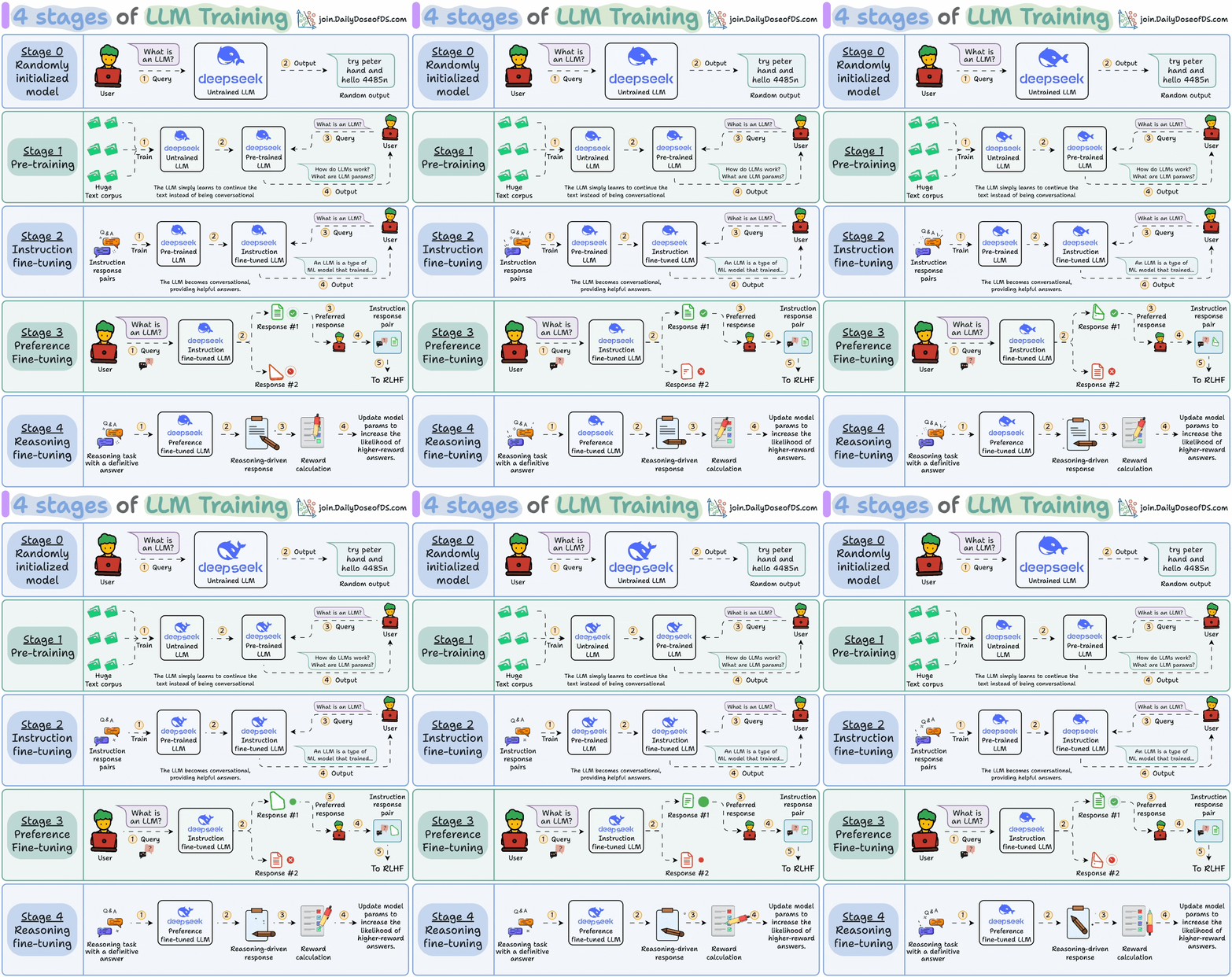
Before Agents: How an LLM Becomes Useful
Pre-train → Instruct → Align → Reason
Source: X
- Pre-training — learn to continue text
- Instruction tuning — learn to follow requests
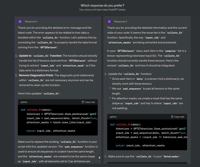
- Preference / RL post-training — learn what responses are preferred
- Reasoning training — learn better problem-solving policies
- The model generates an answer to a prompt.
- The answer is compared to the known correct answer.
- Based on the correctness, we assign a reward. (GRPO)

2026 World Robot Contest (2026.08 Beijing)
# Agent
2023: Generative Agents
Put an LLM inside a world — and let it remember, plan, and act

Generative behavior emerges inside a carefully engineered rule scaffold. 🤫
arXiv:2304.03442 [cs.HC]
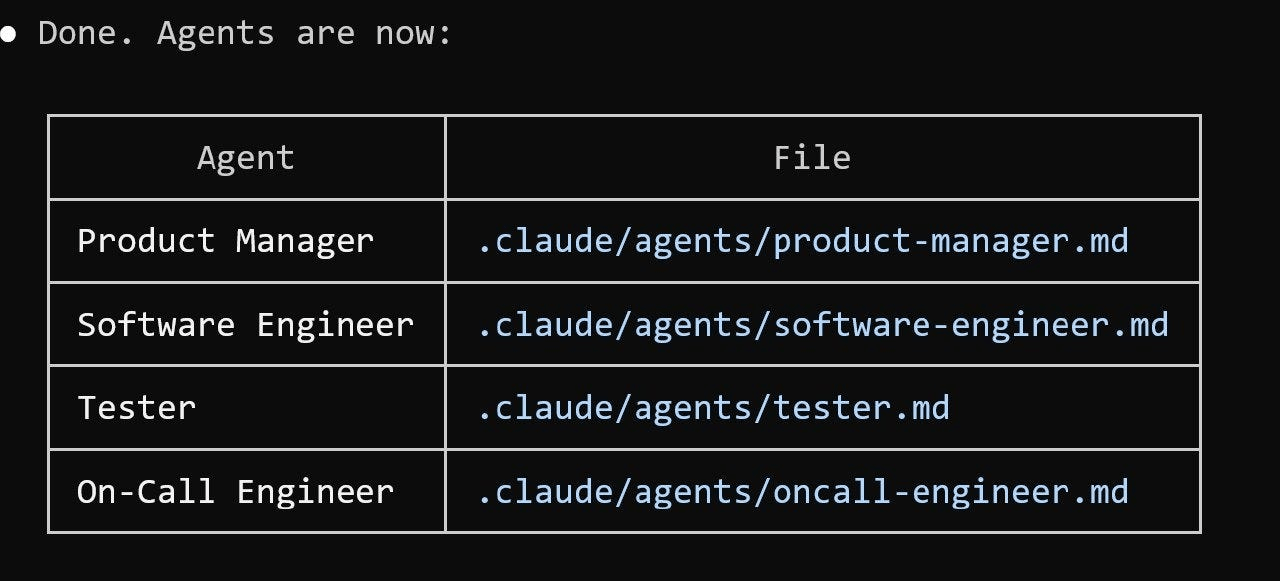
Source: X
Content
-
What Is Machine Learning?
— The basics and why it matters -
Deep Learning: When Machines Start to See and Think
— From neural networks to powerful representations -
Gravitational Waves Meet Machine Learning
— How ML is reshaping data analysis in GW astronomy -
Natural Language Processing
— From transformer to three model families -
From Large Language Models to AI Agents
— Why are LLMs so powerful for automated scientific reasoning? -
Can AI Really Discover?
— From interpolation to search, verification, and science -
Harness Engineering for AI Agents
— How to utilize Claude Code, Codex, ...

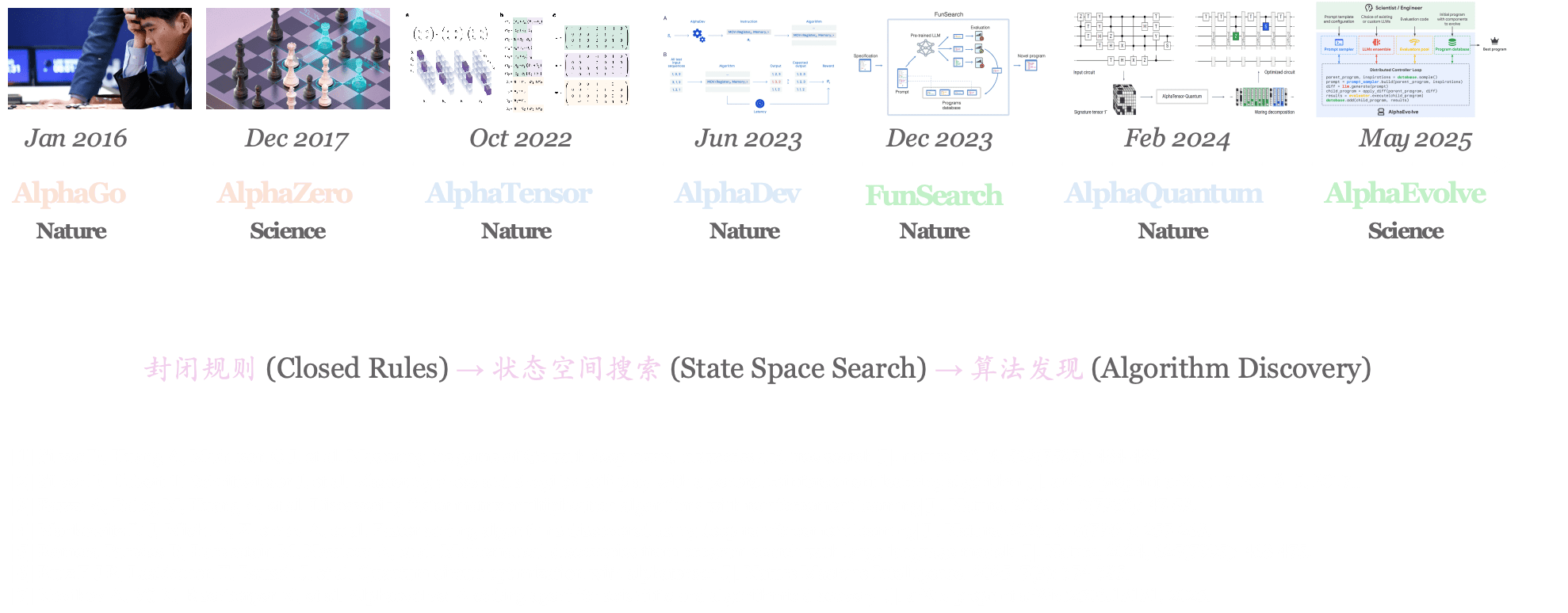
From Game Search to Algorithm Discovery
# Discovery
What changes is not only the model — but the object being searched.

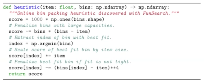
FunSearch: LLM-Guided Search in Program Space
Search for programs that solve the problem, not for the solution itself.

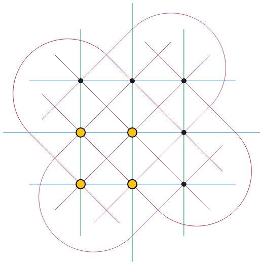
Illustrative example of bin packing using existing heuristic – Best-fit heuristic (left), and using a heuristic discovered by FunSearch (right).
DeepMind Blog (Source)
Cap Set Problem
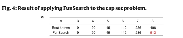
- Given an N, find the maximum number of points that can be found in a grid of dimension N, such that any three points cannot be collinear.
Bin Packing Problem
- How to pack items of different sizes into the minimum number of boxes online.
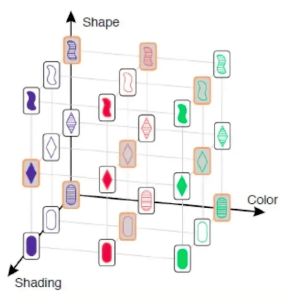
The largets cap set in N=2 has size 4.
The largest cap set in N=3 has size 9 > \(2^3\)
For N > 6, the size of the largest cap set is unknown.
# Discovery
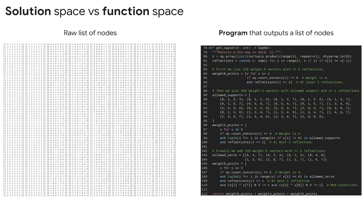
FunSearch: LLM-Guided Search in Program Space
Search for programs that solve the problem, not for the solution itself.
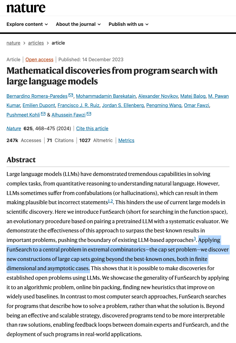
Real-world Case: FunSearch (Nature, 2023)
- LLM + evaluator + evolutionary loop
- Cap set: new constructions beyond previous best-known results
- Online bin packing: improved heuristics over established baselines
- Key idea: discoveries are executable and verifiable
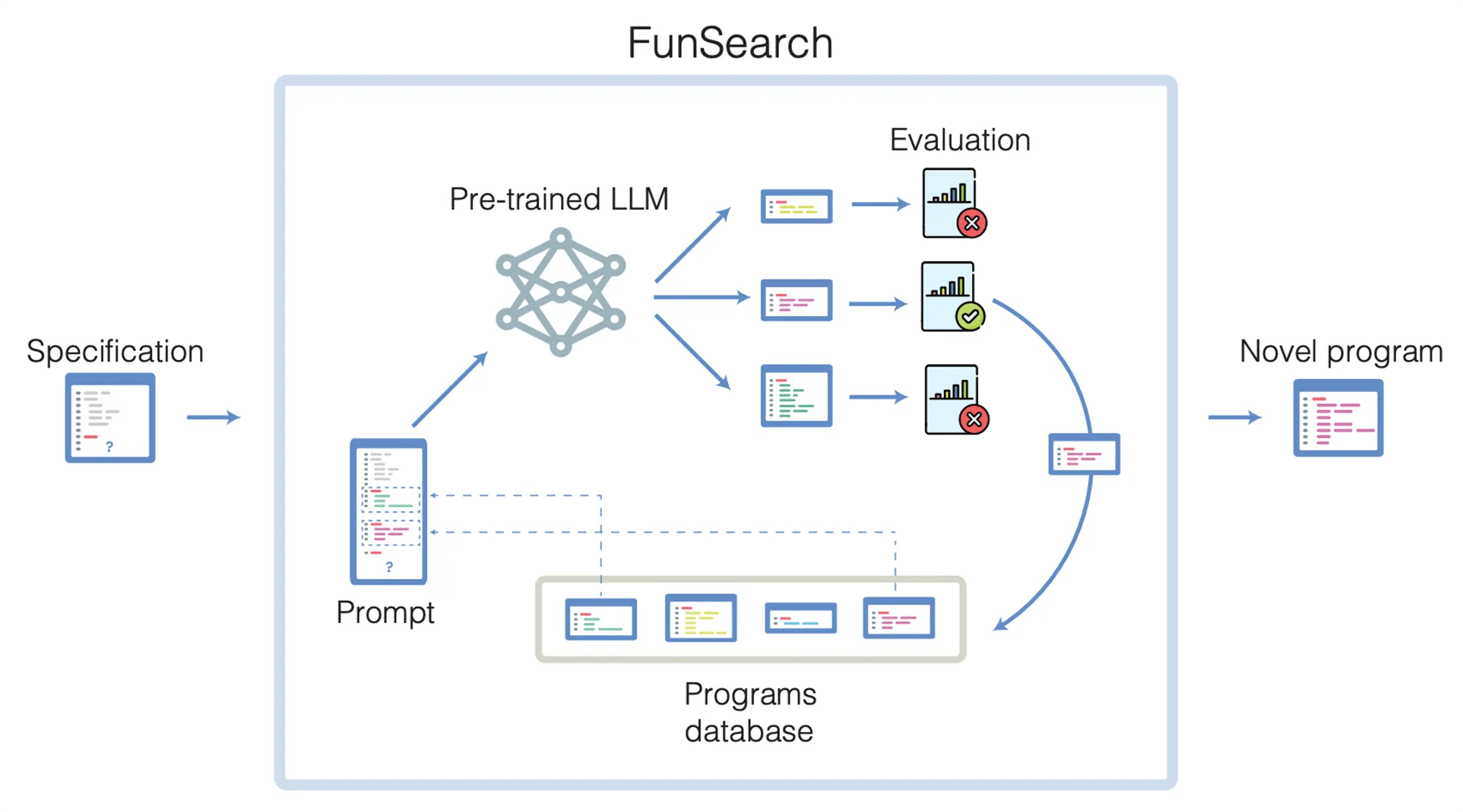
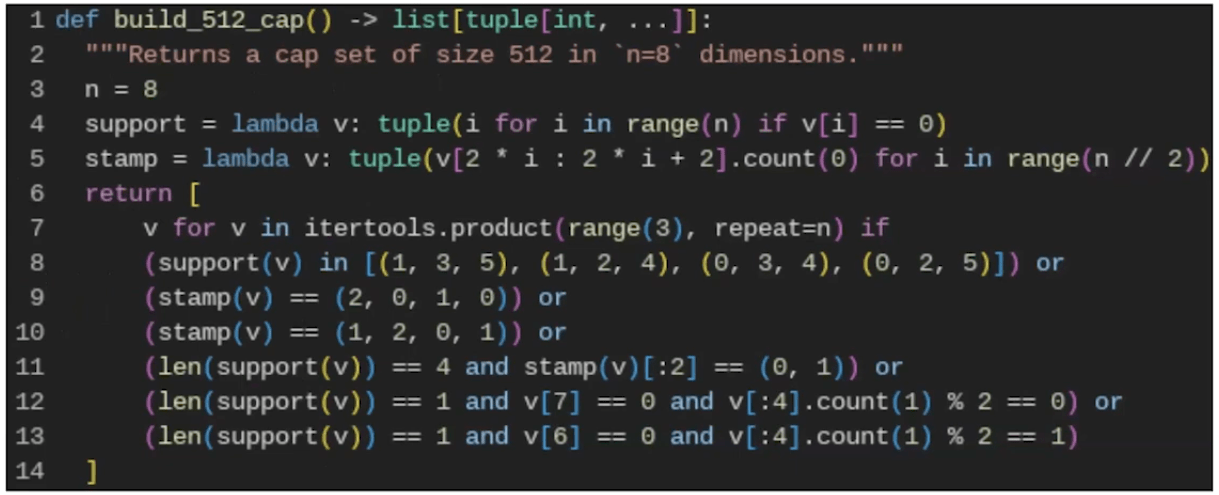
YouTube (Source)
Hallucination becomes exploration when every candidate is externally evaluated.
Generate → Execute → Score → Select → Generate again
# Discovery
FunSearch: LLM-Guided Search in Program Space
Why Search in Program Space?
A solution solves one instance; a program can encode a general strategy.
YouTube (Source)
# Discovery
A New Trend: LLMs as Algorithm Designers
From solving instances to searching for reusable algorithms
The bottleneck moves from generation to search strategy.
Two Directions of LLM-based Optimization
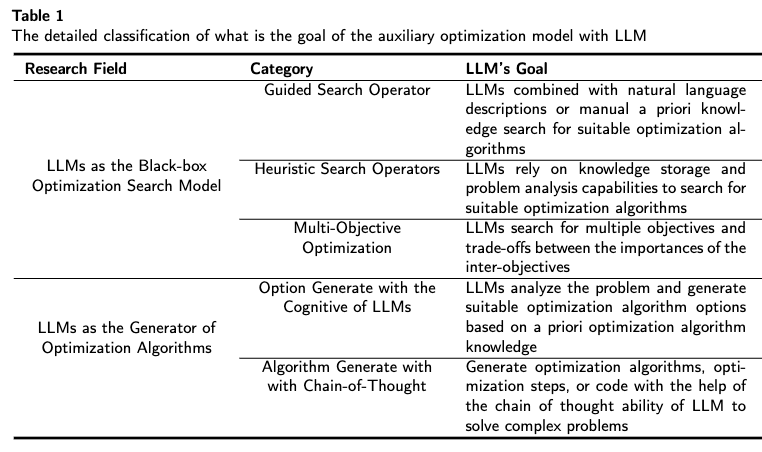
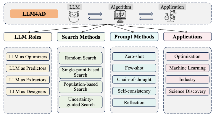
arXiv: 2405.10098 [cs.LG]
arXiv:2410.14716 [cs.LG]
- Direction 1 — LLM as optimizer
- Search directly for a solution
- \(\text{problem instance}\rightarrow\text{LLM}\rightarrow\text{solution}\)
-
Direction 2 — LLM as algorithm designer
-
Search for a heuristic / program / solver
-
\(\text{problem class}\rightarrow\text{LLM + search}\rightarrow\text{algorithm}\rightarrow\text{many instances}\)
-
Much more interesting for scientific discovery.
-
# Discovery
From Evolution to Tree Search
The bottleneck is no longer generating algorithms — it is how to explore the algorithm space.
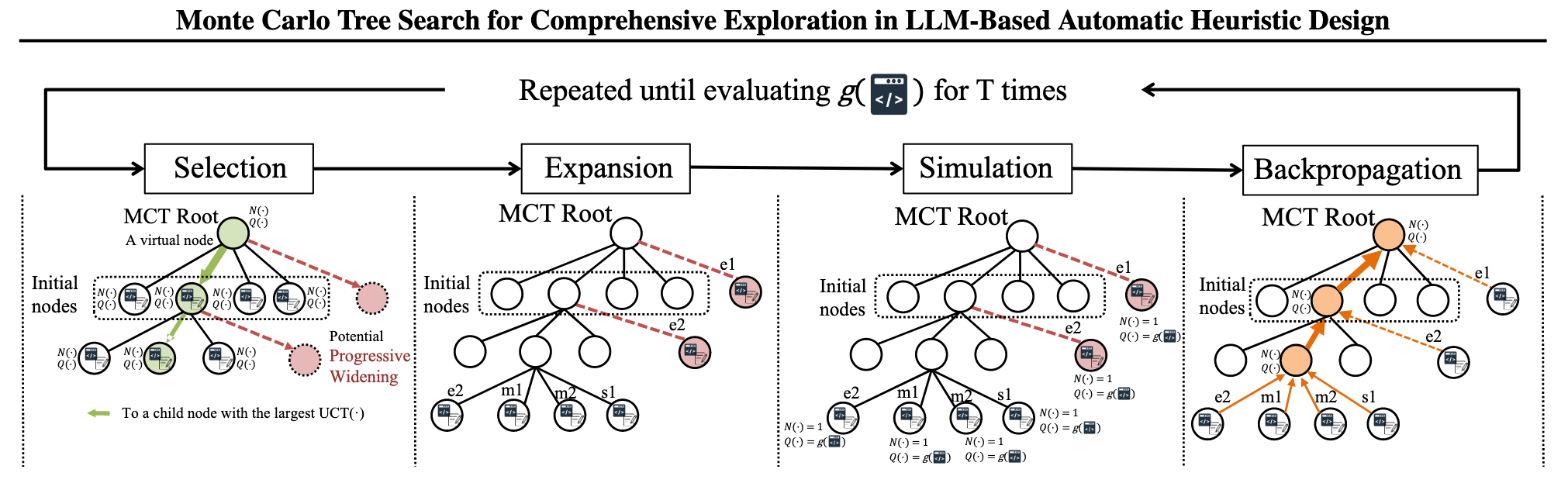
MCTS-AHD
arXiv:2501.08603 [cs.AI]
The search begins to operate not only on code, but also on ideas about why the code works.
Algorithm candidates become nodes in a search tree.
Good branches receive more search budget, while unexplored branches are still sampled.
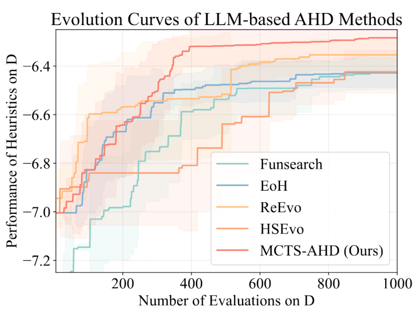
Search organization matters.
arXiv:2402.01145 [cs.NE]
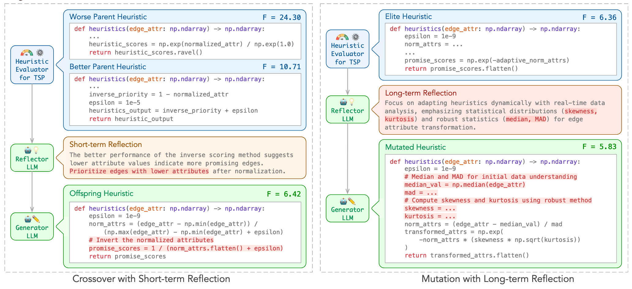
ReEvo
# Discovery
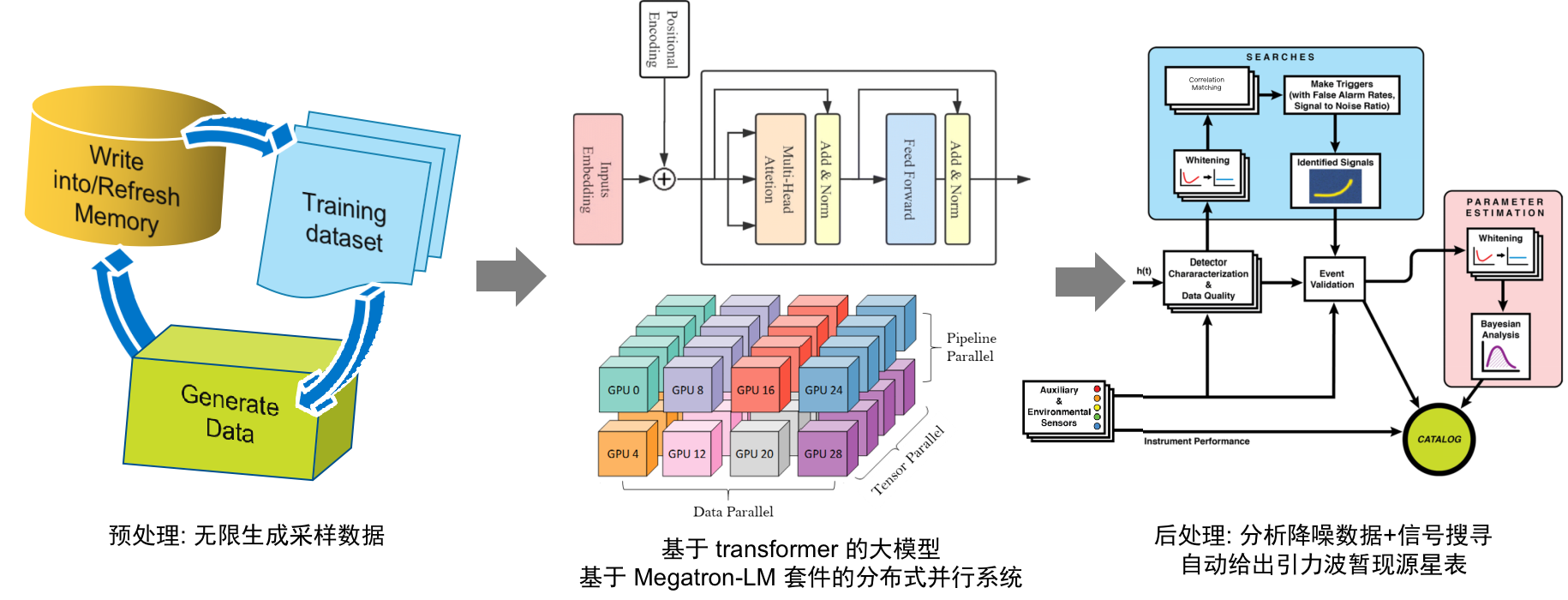
Can LLMs Discover Gravitational Wave Algorithms?
- The Core Shift: Shifting LLMs from predicting data to acting as policies over algorithms
- Loop Mechanism: The LLM proposes candidate code, while an external benchmark (MLGWSC-1) evaluates fitness
- Evo-MCTS Framework: Combining evolutionary search and Monte Carlo Tree Search with test-time compute to discover auditable, high-performance detection pipelines

# Evo-MCTS
Can LLMs Discover Better GW Algorithms?
# Evo-MCTS
The target is not another black-box model — but interpretable, executable analysis logic.
Motivation I — Hand-designed model-based pipelines
- Matched filtering is powerful and interpretable, but often relies on large template banks and carefully engineered assumptions.
- Expanding to broader source classes or non-ideal noise can make the search increasingly expensive and complex.
Motivation II — Black-box data-driven pipelines
- Deep networks can learn flexible nonlinear decision rules directly from data.
- But the learned decision logic is difficult to inspect, validate, and translate into auditable scientific methodology.
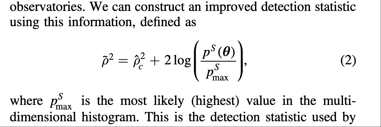
Nitz et al., ApJ (2017)
Sci4MLGW@ICERM (June 2025)
A precedent: improving a classical statistic using learned / empirical prior information
Instead of asking an LLM to detect signals, ask it to discover the detection algorithm.
When LLMs Enter the Algorithmic Loop
# Evo-MCTS
The LLM does not predict answers — it reshapes how we search for algorithms.
The LLM proposes. The benchmark judges.
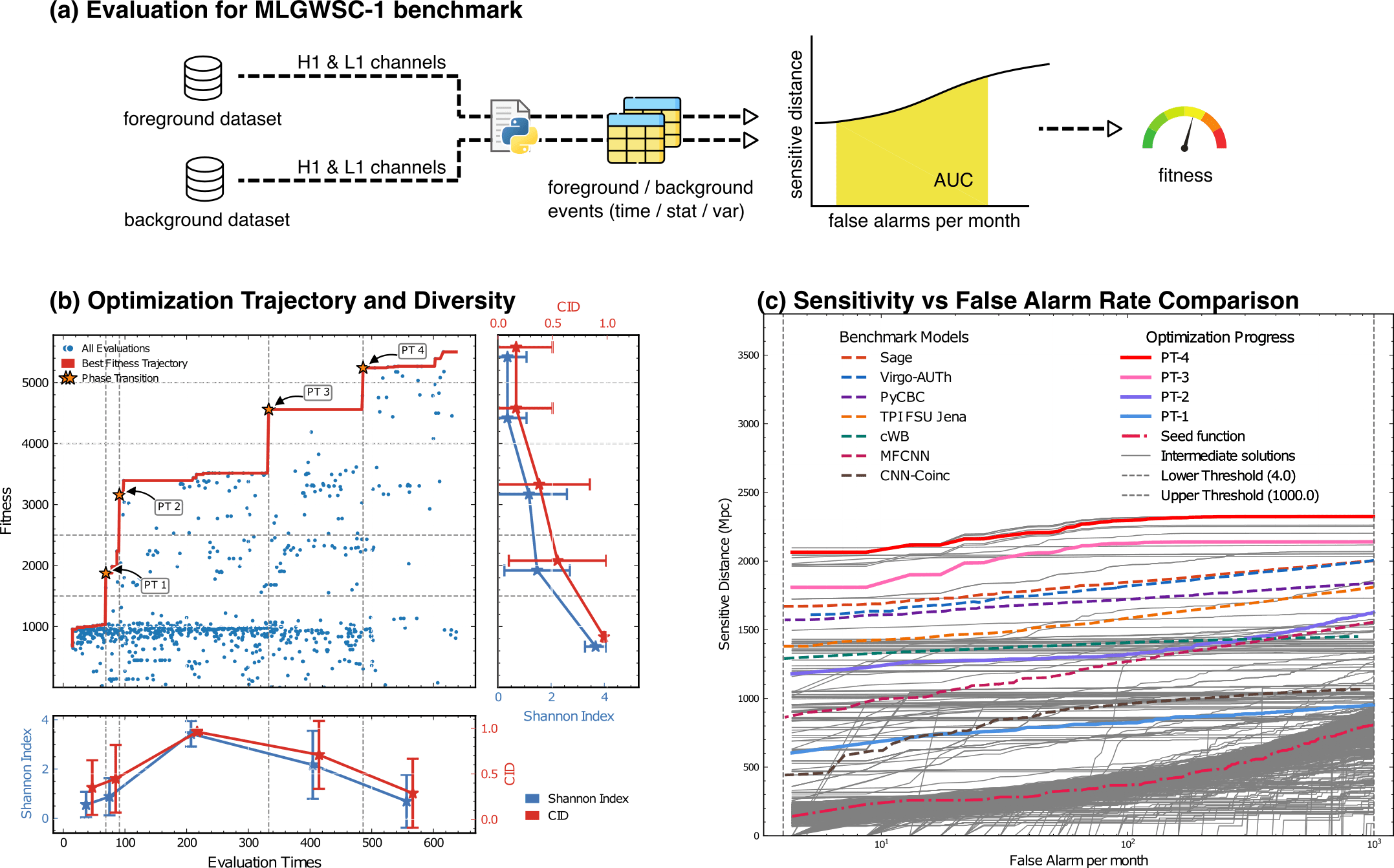
External evaluator: MLGWSC-1
Concept
Mechanism
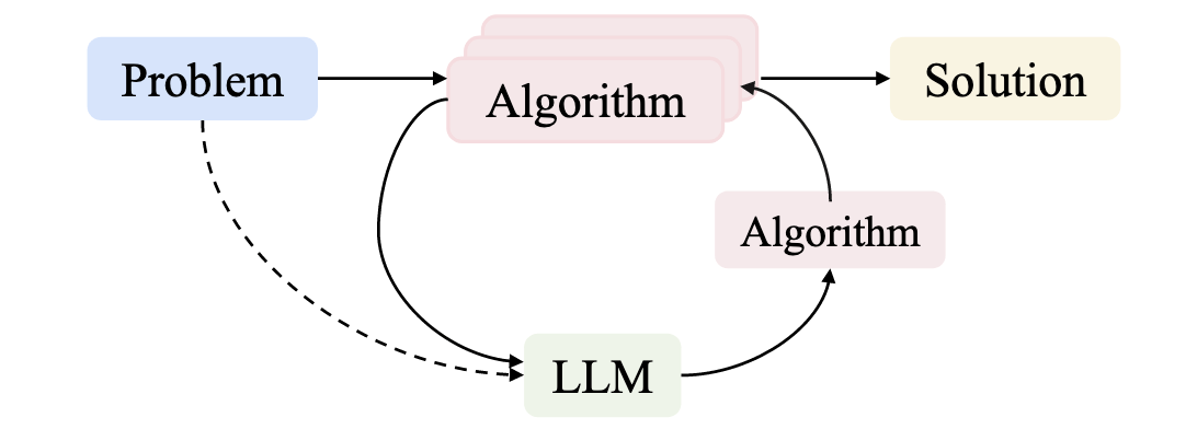
Problem → Algorithm
Benchmark → Algorithm → Fitness
↻ LLM-guided search and refinement
From solving instances to discovering reusable methods
HW, LZ. arXiv:2508.03661 [cs.AI]
From solving instances to discovering reusable methods
When LLMs Enter the Algorithmic Loop
# Evo-MCTS
The LLM does not predict answers — it reshapes how we search for algorithms.
external_knowledge
(constraint)
Execute on benchmark data
LLM as designer
arXiv:2410.14716 [cs.LG]
import numpy as np
import scipy.signal as signal
def pipeline_v1(strain_h1: np.ndarray, strain_l1: np.ndarray, times: np.ndarray) -> tuple[np.ndarray, np.ndarray, np.ndarray]:
    def data_conditioning(strain_h1: np.ndarray, strain_l1: np.ndarray, times: np.ndarray) -> tuple[np.ndarray, np.ndarray, np.ndarray]:
        window_length = 4096
        dt = times[1] - times[0]
        fs = 1.0 / dt

        def whiten_strain(strain):
            strain_zeromean = strain - np.mean(strain)
            freqs, psd = signal.welch(strain_zeromean, fs=fs, nperseg=window_length,
                                       window='hann', noverlap=window_length//2)
            smoothed_psd = np.convolve(psd, np.ones(32) / 32, mode='same')
            smoothed_psd = np.maximum(smoothed_psd, np.finfo(float).tiny)
            white_fft = np.fft.rfft(strain_zeromean) / np.sqrt(np.interp(np.fft.rfftfreq(len(strain_zeromean), d=dt), freqs, smoothed_psd))
            return np.fft.irfft(white_fft)

        whitened_h1 = whiten_strain(strain_h1)
        whitened_l1 = whiten_strain(strain_l1)

        return whitened_h1, whitened_l1, times

    def compute_metric_series(h1_data: np.ndarray, l1_data: np.ndarray, time_series: np.ndarray) -> tuple[np.ndarray, np.ndarray]:
        fs = 1 / (time_series[1] - time_series[0])
        f_h1, t_h1, Sxx_h1 = signal.spectrogram(h1_data, fs=fs, nperseg=256, noverlap=128, mode='magnitude', detrend=False)
        f_l1, t_l1, Sxx_l1 = signal.spectrogram(l1_data, fs=fs, nperseg=256, noverlap=128, mode='magnitude', detrend=False)
        tf_metric = np.mean((Sxx_h1**2 + Sxx_l1**2) / 2, axis=0)
        gps_mid_time = time_series[0] + (time_series[-1] - time_series[0]) / 2
        metric_times = gps_mid_time + (t_h1 - t_h1[-1] / 2)

        return tf_metric, metric_times

    def calculate_statistics(tf_metric, t_h1):
        background_level = np.median(tf_metric)
        peaks, _ = signal.find_peaks(tf_metric, height=background_level * 1.0, distance=2, prominence=background_level * 0.3)
        peak_times = t_h1[peaks]
        peak_heights = tf_metric[peaks]
        peak_deltat = np.full(len(peak_times), 10.0)  # Fixed uncertainty value
        return peak_times, peak_heights, peak_deltat

    whitened_h1, whitened_l1, data_times = data_conditioning(strain_h1, strain_l1, times)
    tf_metric, metric_times = compute_metric_series(whitened_h1, whitened_l1, data_times)
    peak_times, peak_heights, peak_deltat = calculate_statistics(tf_metric, metric_times)

    return peak_times, peak_heights, peak_deltat
Optimization Target: Maximizing Area Under Curve (AUC) over the target false-alarm-rate range (e.g. 1–1000 false alarms/month), balancing detection sensitivity and false alarm rates across algorithm generations
MLGWSC-1 benchmark
HW, LZ. arXiv:2508.03661 [cs.AI]
LLMs act as policies over algorithms, not predictors of data.
When LLMs Enter the Algorithmic Loop
# Evo-MCTS
The LLM does not predict answers — it reshapes how we search for algorithms.
external_knowledge
(constraint)
Execute on benchmark data
LLM as designer
arXiv:2410.14716 [cs.LG]
import numpy as np
import scipy.signal as signal
def pipeline_v1(strain_h1: np.ndarray, strain_l1: np.ndarray, times: np.ndarray) -> tuple[np.ndarray, np.ndarray, np.ndarray]:
    def data_conditioning(strain_h1: np.ndarray, strain_l1: np.ndarray, times: np.ndarray) -> tuple[np.ndarray, np.ndarray, np.ndarray]:
        window_length = 4096
        dt = times[1] - times[0]
        fs = 1.0 / dt

        def whiten_strain(strain):
            strain_zeromean = strain - np.mean(strain)
            freqs, psd = signal.welch(strain_zeromean, fs=fs, nperseg=window_length,
                                       window='hann', noverlap=window_length//2)
            smoothed_psd = np.convolve(psd, np.ones(32) / 32, mode='same')
            smoothed_psd = np.maximum(smoothed_psd, np.finfo(float).tiny)
            white_fft = np.fft.rfft(strain_zeromean) / np.sqrt(np.interp(np.fft.rfftfreq(len(strain_zeromean), d=dt), freqs, smoothed_psd))
            return np.fft.irfft(white_fft)

        whitened_h1 = whiten_strain(strain_h1)
        whitened_l1 = whiten_strain(strain_l1)

        return whitened_h1, whitened_l1, times

    def compute_metric_series(h1_data: np.ndarray, l1_data: np.ndarray, time_series: np.ndarray) -> tuple[np.ndarray, np.ndarray]:
        fs = 1 / (time_series[1] - time_series[0])
        f_h1, t_h1, Sxx_h1 = signal.spectrogram(h1_data, fs=fs, nperseg=256, noverlap=128, mode='magnitude', detrend=False)
        f_l1, t_l1, Sxx_l1 = signal.spectrogram(l1_data, fs=fs, nperseg=256, noverlap=128, mode='magnitude', detrend=False)
        tf_metric = np.mean((Sxx_h1**2 + Sxx_l1**2) / 2, axis=0)
        gps_mid_time = time_series[0] + (time_series[-1] - time_series[0]) / 2
        metric_times = gps_mid_time + (t_h1 - t_h1[-1] / 2)

        return tf_metric, metric_times

    def calculate_statistics(tf_metric, t_h1):
        background_level = np.median(tf_metric)
        peaks, _ = signal.find_peaks(tf_metric, height=background_level * 1.0, distance=2, prominence=background_level * 0.3)
        peak_times = t_h1[peaks]
        peak_heights = tf_metric[peaks]
        peak_deltat = np.full(len(peak_times), 10.0)  # Fixed uncertainty value
        return peak_times, peak_heights, peak_deltat

    whitened_h1, whitened_l1, data_times = data_conditioning(strain_h1, strain_l1, times)
    tf_metric, metric_times = compute_metric_series(whitened_h1, whitened_l1, data_times)
    peak_times, peak_heights, peak_deltat = calculate_statistics(tf_metric, metric_times)

    return peak_times, peak_heights, peak_deltat
HW, LZ. arXiv:2508.03661 [cs.AI]
LLMs act as policies over algorithms, not predictors of data.
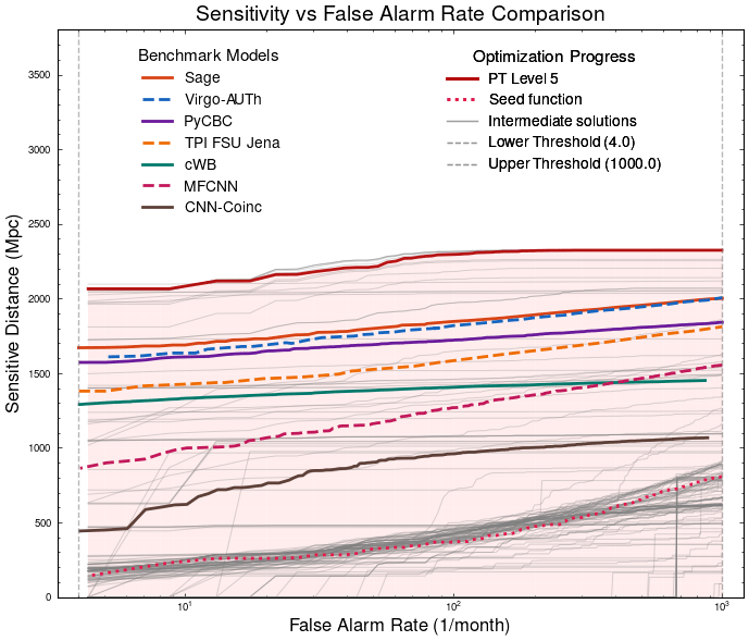
PyCBC (linear-core)
cWB (nonlinear-core)
Simple filters (non-linear)
CNN-like (highly non-linear)
Benchmarking against state-of-the-art methods
When LLMs Enter the Algorithmic Loop
# Evo-MCTS
The LLM does not predict answers — it reshapes how we search for algorithms.
external_knowledge
(constraint)
Execute on benchmark data
LLM as designer
arXiv:2410.14716 [cs.LG]
import numpy as np
import scipy.signal as signal
def pipeline_v1(strain_h1: np.ndarray, strain_l1: np.ndarray, times: np.ndarray) -> tuple[np.ndarray, np.ndarray, np.ndarray]:
    def data_conditioning(strain_h1: np.ndarray, strain_l1: np.ndarray, times: np.ndarray) -> tuple[np.ndarray, np.ndarray, np.ndarray]:
        window_length = 4096
        dt = times[1] - times[0]
        fs = 1.0 / dt

        def whiten_strain(strain):
            strain_zeromean = strain - np.mean(strain)
            freqs, psd = signal.welch(strain_zeromean, fs=fs, nperseg=window_length,
                                       window='hann', noverlap=window_length//2)
            smoothed_psd = np.convolve(psd, np.ones(32) / 32, mode='same')
            smoothed_psd = np.maximum(smoothed_psd, np.finfo(float).tiny)
            white_fft = np.fft.rfft(strain_zeromean) / np.sqrt(np.interp(np.fft.rfftfreq(len(strain_zeromean), d=dt), freqs, smoothed_psd))
            return np.fft.irfft(white_fft)

        whitened_h1 = whiten_strain(strain_h1)
        whitened_l1 = whiten_strain(strain_l1)

        return whitened_h1, whitened_l1, times

    def compute_metric_series(h1_data: np.ndarray, l1_data: np.ndarray, time_series: np.ndarray) -> tuple[np.ndarray, np.ndarray]:
        fs = 1 / (time_series[1] - time_series[0])
        f_h1, t_h1, Sxx_h1 = signal.spectrogram(h1_data, fs=fs, nperseg=256, noverlap=128, mode='magnitude', detrend=False)
        f_l1, t_l1, Sxx_l1 = signal.spectrogram(l1_data, fs=fs, nperseg=256, noverlap=128, mode='magnitude', detrend=False)
        tf_metric = np.mean((Sxx_h1**2 + Sxx_l1**2) / 2, axis=0)
        gps_mid_time = time_series[0] + (time_series[-1] - time_series[0]) / 2
        metric_times = gps_mid_time + (t_h1 - t_h1[-1] / 2)

        return tf_metric, metric_times

    def calculate_statistics(tf_metric, t_h1):
        background_level = np.median(tf_metric)
        peaks, _ = signal.find_peaks(tf_metric, height=background_level * 1.0, distance=2, prominence=background_level * 0.3)
        peak_times = t_h1[peaks]
        peak_heights = tf_metric[peaks]
        peak_deltat = np.full(len(peak_times), 10.0)  # Fixed uncertainty value
        return peak_times, peak_heights, peak_deltat

    whitened_h1, whitened_l1, data_times = data_conditioning(strain_h1, strain_l1, times)
    tf_metric, metric_times = compute_metric_series(whitened_h1, whitened_l1, data_times)
    peak_times, peak_heights, peak_deltat = calculate_statistics(tf_metric, metric_times)

    return peak_times, peak_heights, peak_deltat
HW, LZ. arXiv:2508.03661 [cs.AI]
LLMs act as policies over algorithms, not predictors of data.
PyCBC (linear-core)
cWB (nonlinear-core)
Simple filters (non-linear)
CNN-like (highly non-linear)
Benchmarking against state-of-the-art methods
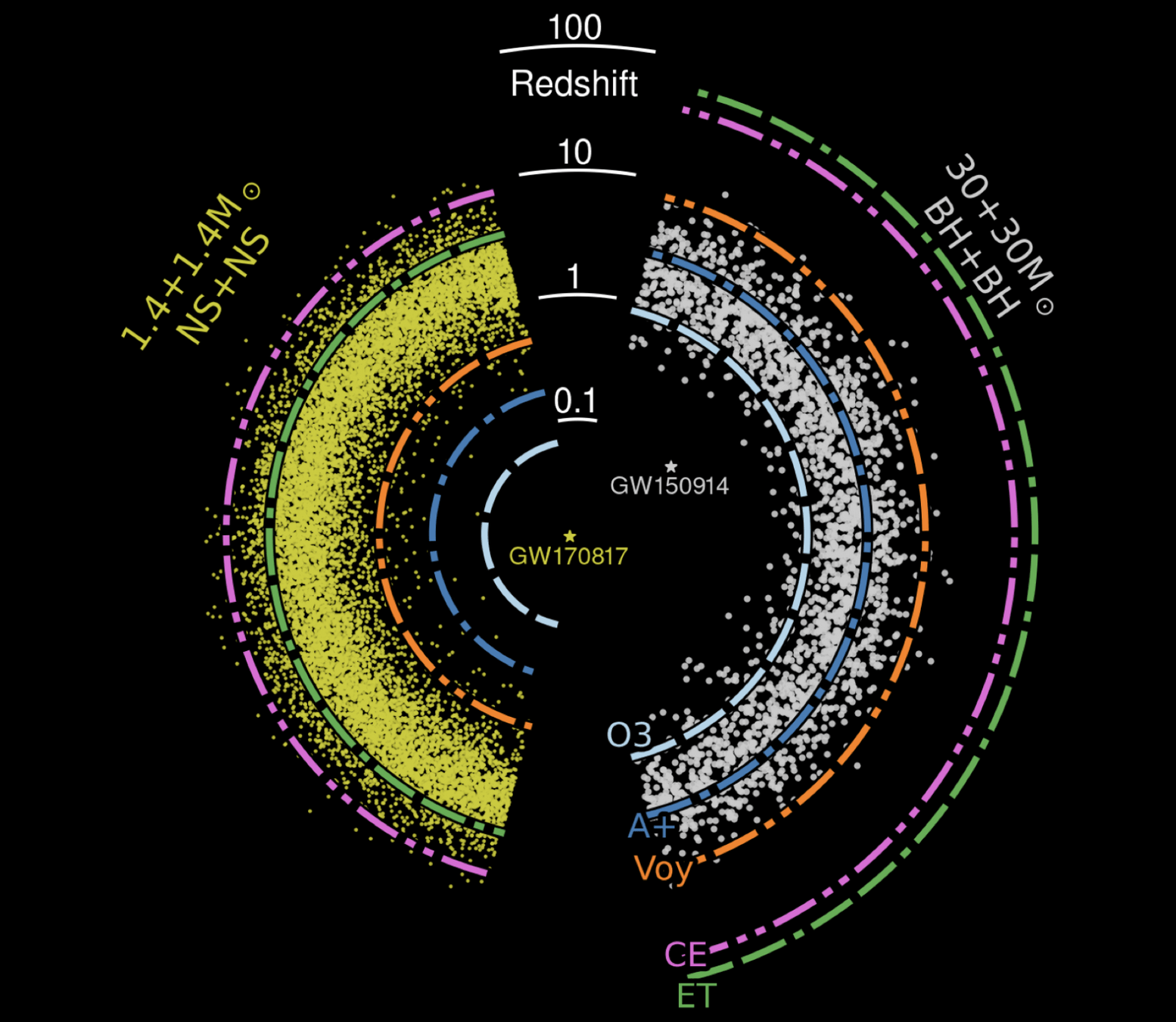
When LLMs Enter the Algorithmic Loop
# Evo-MCTS
The LLM does not predict answers — it reshapes how we search for algorithms.
external_knowledge
(constraint)
LLM as designer
arXiv:2410.14716 [cs.LG]
HW, LZ. arXiv:2508.03661 [cs.AI]
LLMs act as policies over algorithms, not predictors of data.
You are an expert in gravitational wave signal detection algorithms. Your task is to design heuristics that can effectively solve optimization problems.

{prompt_task}

I have analyzed two algorithms and provided a reflection on their differences.

[Worse code]
{worse_code}

[Better code]
{better_code}

[Reflection]
{reflection}

{external_knowledge}

Based on this reflection, please write an improved algorithm according to the reflection.
First, describe the design idea and main steps of your algorithm in one sentence. The description must be inside a brace outside the code implementation. Next, implement it in Python as a function named '{func_name}'.
This function should accept {input_count} input(s): {joined_inputs}. The function should return {output_count} output(s): {joined_outputs}.
{inout_inf} {other_inf}

Do not give additional explanations.
One Prompt Template for MLGWSC1 Algorithm Synthesis
Evo-MCTS: Searching for Interpretable GW Algorithms
# Evo-MCTS
Tree search over LLM-generated algorithms
external_knowledge
(constraint)
LLM as designer
arXiv:2410.14716 [cs.LG]
HW, LZ. arXiv:2508.03661 [cs.AI]
LLMs act as policies over algorithms, not predictors of data.
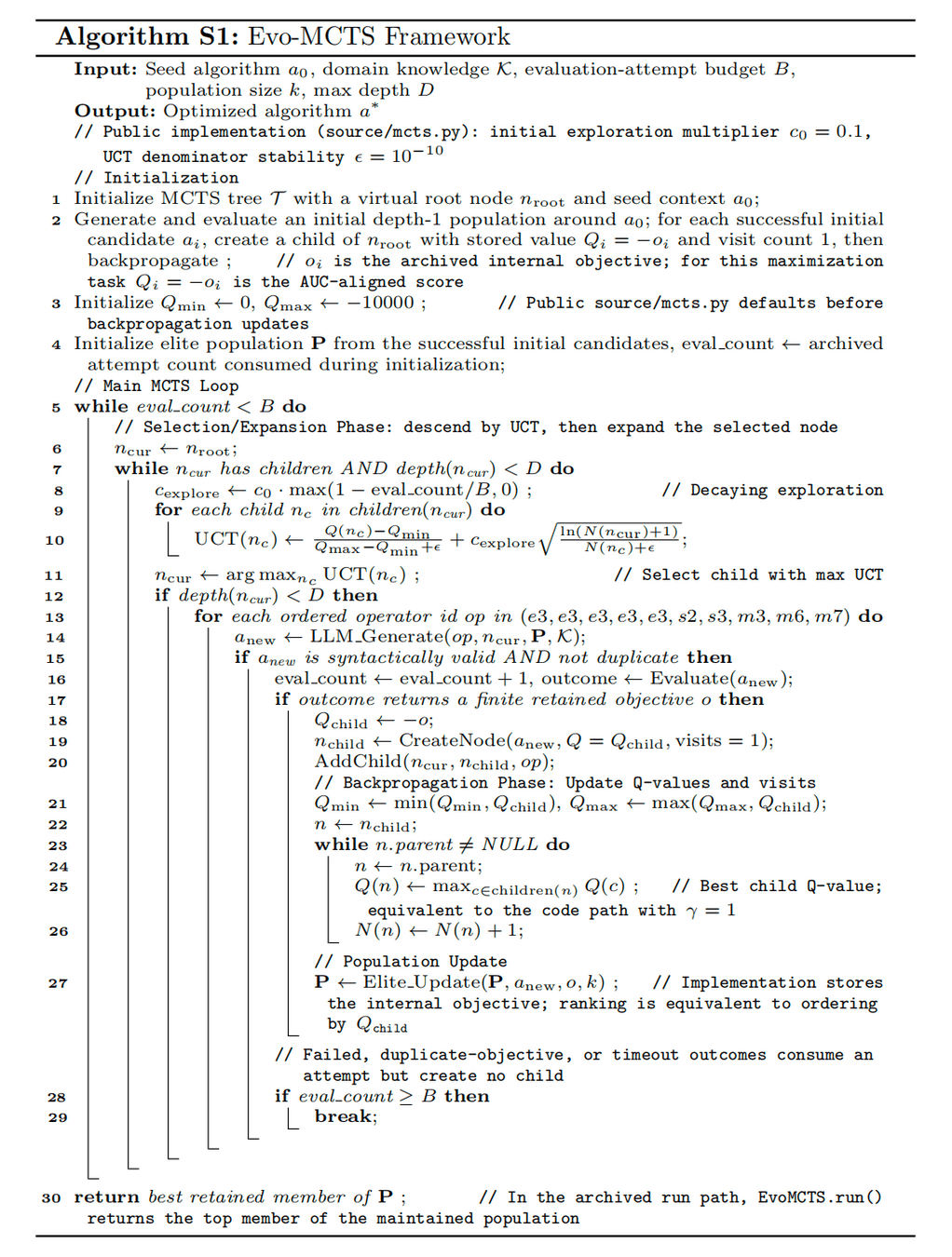
From Scaling to Search: Why MCTS Comes Back
# Evo-MCTS
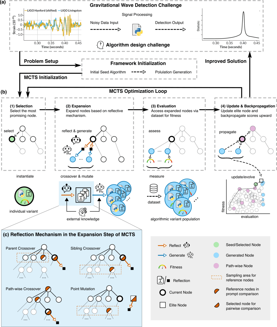
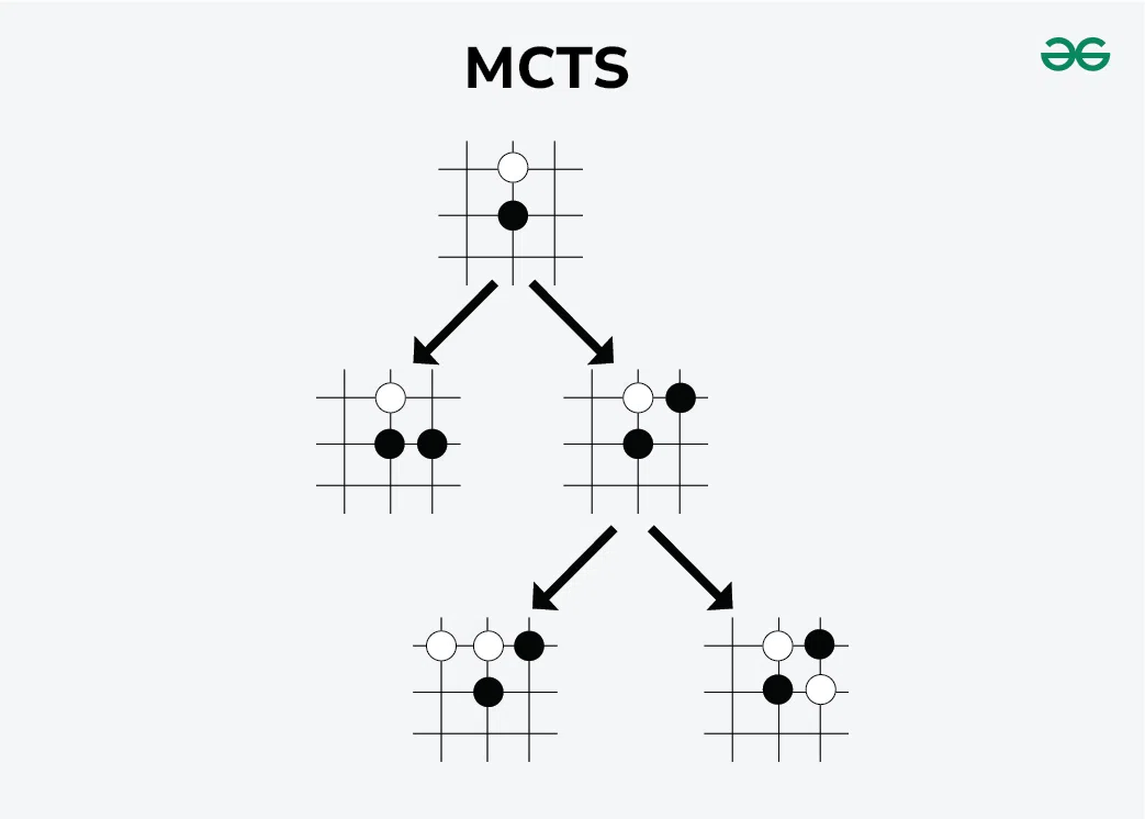
MCTS
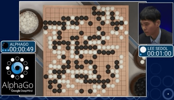
Casse1: Go Game
Case 2: Reasoning models and test-time compute
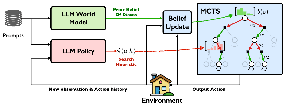
The release of o1 marks the formal deployment of the inference-time scaling paradigm in production. As Richard Sutton pointed out in The Bitter Lesson, only learning and search are methods that can scale indefinitely with compute. From this point on, the focus has increasingly shifted toward search.
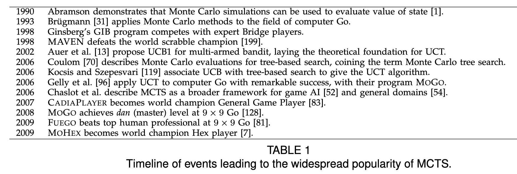
Browne et al. (2012)
arXiv:2305.14078 [cs.RO]
Monte Carlo Tree Search (MCTS), which allocates computation to promising branches while preserving exploration, has long been a core technique in modern game-playing systems such as AlphaGo.
LLM-Informed Evo-MCTS
Why Evolution? Diversity for Algorithm Search
# Evo-MCTS
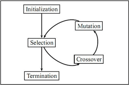
LLM-Informed Evo-MCTS
EA
Evolution proposes diverse variants; MCTS decides where to spend search budget.
Evolutionary Algorithms (EAs) provide:
- Diversity — explore multiple algorithmic directions
- Gradient-free search — suitable for discrete program spaces
- Variation operators — mutation and crossover generate novel candidates
They are especially natural when the search object is executable code.
Population-level search
Evolution creates diversity; MCTS allocates attention.
LLM makes the variation semantic rather than random.
When LLMs Enter the Algorithmic Loop
# Evo-MCTS
The LLM does not predict answers — it reshapes how we search for algorithms.
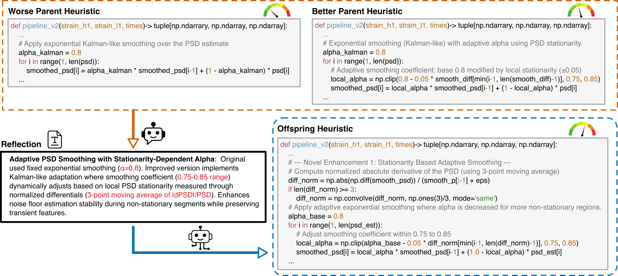
Reflection-Guided Code Evolution
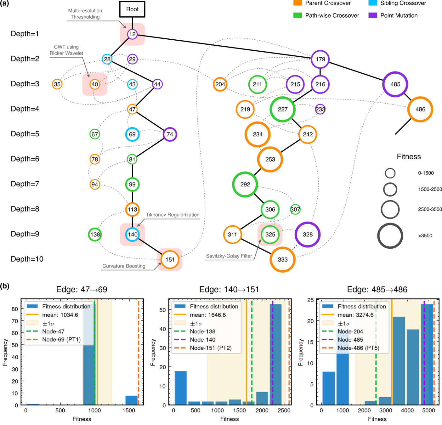
Evo-MCTS Search Trajectory
What changed?
-
LLMs propose actions that guide the search
-
Past evaluations become structured search memory
-
Search history conditions future algorithm generation
- deepseek-R1 for reflection generation
- o3-mini-medium for code generation
HW, LZ. arXiv:2508.03661 [cs.AI]
- node = candidate algorithm
- edge = evolutionary / LLM-guided modification
- size = fitness
Compare → Reflect → Rewrite → Evaluate
Search trajectories matter more than isolated optima.
From Performance to Scientific Understanding
# Evo-MCTS
What did the discovered algorithm actually learn to do?
HW, LZ. arXiv:2508.03661 [cs.AI]
Algorithmic Component Impact Analysis.
- A comprehensive technique impact analysis using controlled comparative methodology
import numpy as np
import scipy.signal as signal
from scipy.signal.windows import tukey
from scipy.signal import savgol_filter

def pipeline_v2(strain_h1: np.ndarray, strain_l1: np.ndarray, times: np.ndarray) -> tuple[np.ndarray, np.ndarray, np.ndarray]:
    """
    The pipeline function processes gravitational wave data from the H1 and L1 detectors to identify potential gravitational wave signals.
    It takes strain_h1 and strain_l1 numpy arrays containing detector data, and times array with corresponding time points.
    The function returns a tuple of three numpy arrays: peak_times containing GPS times of identified events,
    peak_heights with significance values of each peak, and peak_deltat showing time window uncertainty for each peak.
    """
    eps = np.finfo(float).tiny
    dt = times[1] - times[0]
    fs = 1.0 / dt
    # Base spectrogram parameters
    base_nperseg = 256
    base_noverlap = base_nperseg // 2
    medfilt_kernel = 101       # odd kernel size for robust detrending
    uncertainty_window = 5     # half-window for local timing uncertainty

    # -------------------- Stage 1: Robust Baseline Detrending --------------------
    # Remove long-term trends using a median filter for each channel.
    detrended_h1 = strain_h1 - signal.medfilt(strain_h1, kernel_size=medfilt_kernel)
    detrended_l1 = strain_l1 - signal.medfilt(strain_l1, kernel_size=medfilt_kernel)

    # -------------------- Stage 2: Adaptive Whitening with Enhanced PSD Smoothing --------------------
    def adaptive_whitening(strain: np.ndarray) -> np.ndarray:
        # Center the signal.
        centered = strain - np.mean(strain)
        n_samples = len(centered)
        # Adaptive window length: between 5 and 30 seconds
        win_length_sec = np.clip(n_samples / fs / 20, 5, 30)
        nperseg_adapt = int(win_length_sec * fs)
        nperseg_adapt = max(10, min(nperseg_adapt, n_samples))

        # Create a Tukey window with 75% overlap.
        tukey_alpha = 0.25
        win = tukey(nperseg_adapt, alpha=tukey_alpha)
        noverlap_adapt = int(nperseg_adapt * 0.75)
        if noverlap_adapt >= nperseg_adapt:
            noverlap_adapt = nperseg_adapt - 1

        # Estimate the power spectral density (PSD) using Welch's method.
        freqs, psd = signal.welch(centered, fs=fs, nperseg=nperseg_adapt,
                                  noverlap=noverlap_adapt, window=win, detrend='constant')
        psd = np.maximum(psd, eps)

        # Compute relative differences for PSD stationarity measure.
        diff_arr = np.abs(np.diff(psd)) / (psd[:-1] + eps)
        # Smooth the derivative with a moving average.
        if len(diff_arr) >= 3:
            smooth_diff = np.convolve(diff_arr, np.ones(3)/3, mode='same')
        else:
            smooth_diff = diff_arr

        # Exponential smoothing (Kalman-like) with adaptive alpha using PSD stationarity.
        smoothed_psd = np.copy(psd)
        for i in range(1, len(psd)):
            # Adaptive smoothing coefficient: base 0.8 modified by local stationarity (±0.05)
            local_alpha = np.clip(0.8 - 0.05 * smooth_diff[min(i-1, len(smooth_diff)-1)], 0.75, 0.85)
            smoothed_psd[i] = local_alpha * smoothed_psd[i-1] + (1 - local_alpha) * psd[i]

        # Compute Tikhonov regularization gain based on deviation from median PSD.
        noise_baseline = np.median(smoothed_psd)
        raw_gain = (smoothed_psd / (noise_baseline + eps)) - 1.0

        # Compute a causal-like gradient using the Savitzky-Golay filter.
        win_len = 11 if len(smoothed_psd) >= 11 else ((len(smoothed_psd)//2)*2+1)
        polyorder = 2 if win_len > 2 else 1
        delta_freq = np.mean(np.diff(freqs))
        grad_psd = savgol_filter(smoothed_psd, win_len, polyorder, deriv=1, delta=delta_freq, mode='interp')

        # Nonlinear scaling via sigmoid to enhance gradient differences.
        sigmoid = lambda x: 1.0 / (1.0 + np.exp(-x))
        scaling_factor = 1.0 + 2.0 * sigmoid(np.abs(grad_psd) / (np.median(smoothed_psd) + eps))

        # Compute adaptive gain factors with nonlinear scaling.
        gain = 1.0 - np.exp(-0.5 * scaling_factor * raw_gain)
        gain = np.clip(gain, -8.0, 8.0)

        # FFT-based whitening: interpolate gain and PSD onto FFT frequency bins.
        signal_fft = np.fft.rfft(centered)
        freq_bins = np.fft.rfftfreq(n_samples, d=dt)
        interp_gain = np.interp(freq_bins, freqs, gain, left=gain[0], right=gain[-1])
        interp_psd = np.interp(freq_bins, freqs, smoothed_psd, left=smoothed_psd[0], right=smoothed_psd[-1])
        denom = np.sqrt(interp_psd) * (np.abs(interp_gain) + eps)
        denom = np.maximum(denom, eps)
        white_fft = signal_fft / denom
        whitened = np.fft.irfft(white_fft, n=n_samples)
        return whitened

    # Whiten H1 and L1 channels using the adapted method.
    white_h1 = adaptive_whitening(detrended_h1)
    white_l1 = adaptive_whitening(detrended_l1)

    # -------------------- Stage 3: Coherent Time-Frequency Metric with Frequency-Conditioned Regularization --------------------
    def compute_coherent_metric(w1: np.ndarray, w2: np.ndarray) -> tuple[np.ndarray, np.ndarray]:
        # Compute complex spectrograms preserving phase information.
        f1, t_spec, Sxx1 = signal.spectrogram(w1, fs=fs, nperseg=base_nperseg,
                                              noverlap=base_noverlap, mode='complex', detrend=False)
        f2, t_spec2, Sxx2 = signal.spectrogram(w2, fs=fs, nperseg=base_nperseg,
                                               noverlap=base_noverlap, mode='complex', detrend=False)
        # Ensure common time axis length.
        common_len = min(len(t_spec), len(t_spec2))
        t_spec = t_spec[:common_len]
        Sxx1 = Sxx1[:, :common_len]
        Sxx2 = Sxx2[:, :common_len]

        # Compute phase differences and coherence between detectors.
        phase_diff = np.angle(Sxx1) - np.angle(Sxx2)
        phase_coherence = np.abs(np.cos(phase_diff))

        # Estimate median PSD per frequency bin from the spectrograms.
        psd1 = np.median(np.abs(Sxx1)**2, axis=1)
        psd2 = np.median(np.abs(Sxx2)**2, axis=1)

        # Frequency-conditioned regularization gain (reflection-guided).
        lambda_f = 0.5 * ((np.median(psd1) / (psd1 + eps)) + (np.median(psd2) / (psd2 + eps)))
        lambda_f = np.clip(lambda_f, 1e-4, 1e-2)
        # Regularization denominator integrating detector PSDs and lambda.
        reg_denom = (psd1[:, None] + psd2[:, None] + lambda_f[:, None] + eps)

        # Weighted phase coherence that balances phase alignment with noise levels.
        weighted_comp = phase_coherence / reg_denom

        # Compute axial (frequency) second derivatives as curvature estimates.
        d2_coh = np.gradient(np.gradient(phase_coherence, axis=0), axis=0)
        avg_curvature = np.mean(np.abs(d2_coh), axis=0)

        # Nonlinear activation boost using tanh for regions of high curvature.
        nonlinear_boost = np.tanh(5 * avg_curvature)
        linear_boost = 1.0 + 0.1 * avg_curvature

        # Cross-detector synergy: weight derived from global median consistency.
        novel_weight = np.mean((np.median(psd1) + np.median(psd2)) / (psd1[:, None] + psd2[:, None] + eps), axis=0)

        # Integrated time-frequency metric combining all enhancements.
        tf_metric = np.sum(weighted_comp * linear_boost * (1.0 + nonlinear_boost), axis=0) * novel_weight

        # Adjust the spectrogram time axis to account for window delay.
        metric_times = t_spec + times[0] + (base_nperseg / 2) / fs
        return tf_metric, metric_times

    tf_metric, metric_times = compute_coherent_metric(white_h1, white_l1)

    # -------------------- Stage 4: Multi-Resolution Thresholding with Octave-Spaced Dyadic Wavelet Validation --------------------
    def multi_resolution_thresholding(metric: np.ndarray, times_arr: np.ndarray) -> tuple[np.ndarray, np.ndarray, np.ndarray]:
        # Robust background estimation with median and MAD.
        bg_level = np.median(metric)
        mad_val = np.median(np.abs(metric - bg_level))
        robust_std = 1.4826 * mad_val
        threshold = bg_level + 1.5 * robust_std

        # Identify candidate peaks using prominence and minimum distance criteria.
        peaks, _ = signal.find_peaks(metric, height=threshold, distance=2, prominence=0.8 * robust_std)
        if peaks.size == 0:
            return np.array([]), np.array([]), np.array([])

        # Local uncertainty estimation using a Gaussian-weighted convolution.
        win_range = np.arange(-uncertainty_window, uncertainty_window + 1)
        sigma = uncertainty_window / 2.5
        gauss_kernel = np.exp(-0.5 * (win_range / sigma) ** 2)
        gauss_kernel /= np.sum(gauss_kernel)
        weighted_mean = np.convolve(metric, gauss_kernel, mode='same')
        weighted_sq = np.convolve(metric ** 2, gauss_kernel, mode='same')
        variances = np.maximum(weighted_sq - weighted_mean ** 2, 0.0)
        uncertainties = np.sqrt(variances)
        uncertainties = np.maximum(uncertainties, 0.01)

        valid_times = []
        valid_heights = []
        valid_uncerts = []
        n_metric = len(metric)

        # Compute a simple second derivative for local curvature checking.
        if n_metric > 2:
            second_deriv = np.diff(metric, n=2)
            second_deriv = np.pad(second_deriv, (1, 1), mode='edge')
        else:
            second_deriv = np.zeros_like(metric)

        # Use octave-spaced scales (dyadic wavelet validation) to validate peak significance.
        widths = np.arange(1, 9)  # approximate scales 1 to 8
        for peak in peaks:
            # Skip peaks lacking sufficient negative curvature.
            if second_deriv[peak] > -0.1 * robust_std:
                continue
            local_start = max(0, peak - uncertainty_window)
            local_end = min(n_metric, peak + uncertainty_window + 1)
            local_segment = metric[local_start:local_end]
            if len(local_segment) < 3:
                continue
            try:
                cwt_coeff = signal.cwt(local_segment, signal.ricker, widths)
            except Exception:
                continue
            max_coeff = np.max(np.abs(cwt_coeff))
            # Threshold for validating the candidate using local MAD.
            cwt_thresh = mad_val * np.sqrt(2 * np.log(len(local_segment) + eps))
            if max_coeff >= cwt_thresh:
                valid_times.append(times_arr[peak])
                valid_heights.append(metric[peak])
                valid_uncerts.append(uncertainties[peak])

        if len(valid_times) == 0:
            return np.array([]), np.array([]), np.array([])
        return np.array(valid_times), np.array(valid_heights), np.array(valid_uncerts)

    peak_times, peak_heights, peak_deltat = multi_resolution_thresholding(tf_metric, metric_times)
return peak_times, peak_heights, peak_deltat- Automatically discover and interpret the value of nonlinear algorithms
- Facilitating new knowledge production along with experience guidance
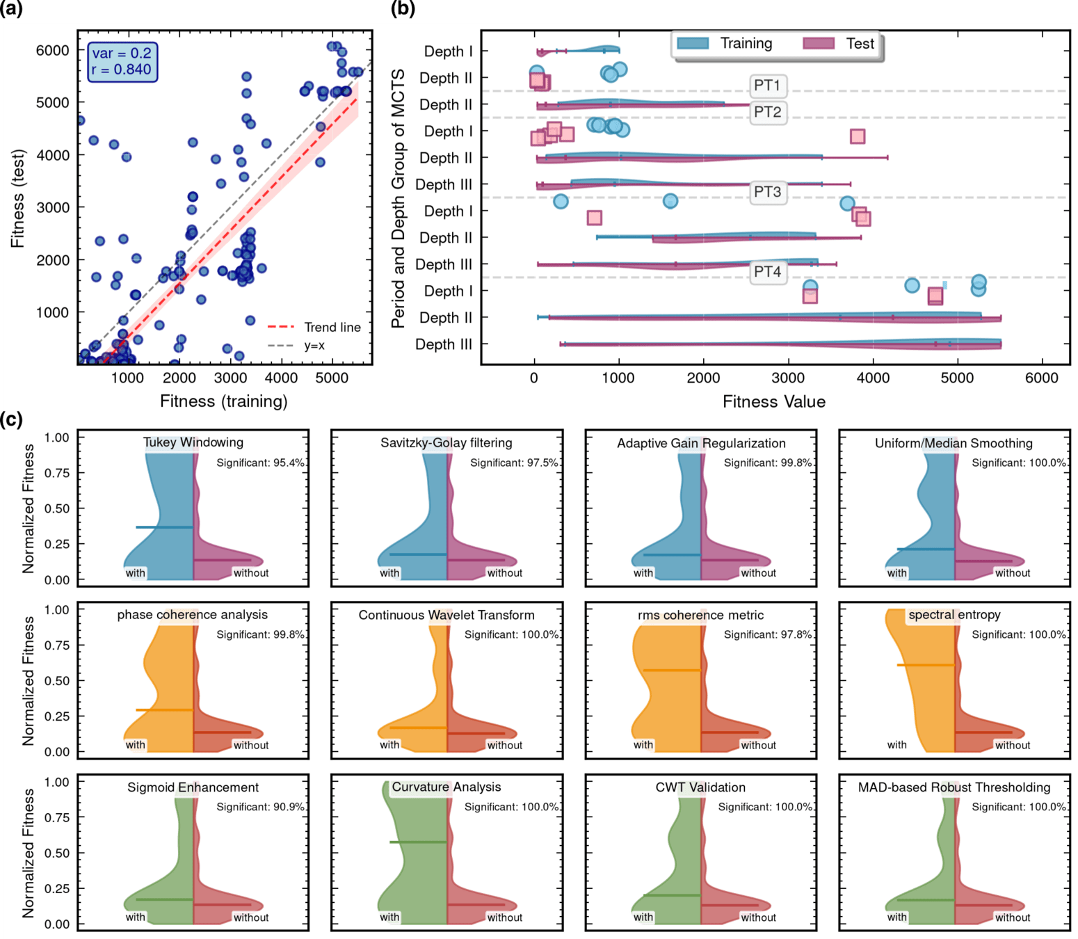
Why Does Evo-MCTS Work?
# Evo-MCTS
Architecture, model choice, and external knowledge each contribute differently.
HW, LZ. arXiv:2508.03661 [cs.AI]
1. Does the integrated search architecture matter?
- Compare the full Evo-MCTS framework with constituent search strategies operating separately.
- Evo-MCTS — MCTS + evolutionary operators + reflection
- MCTS-AHD — tree-search-based AHD
- ReEvo — evolution + reflection
3. Does prior scientific knowledge help?
- Compare search with vs. without external domain knowledge
- non-linear vs linear only
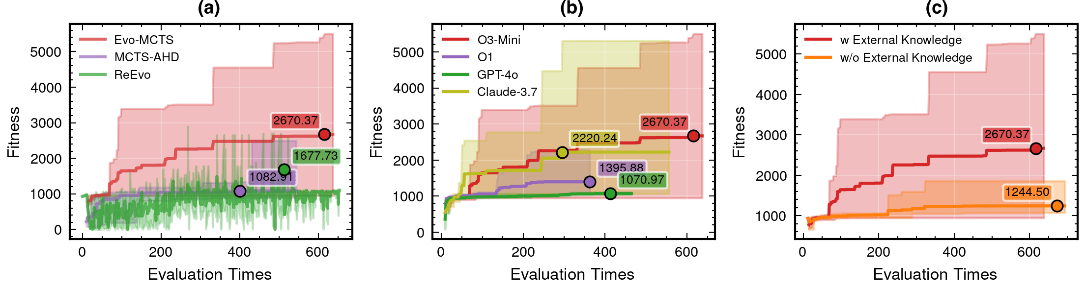
2. How much does the choice of LLM matter?
- Replace the code-generation / reflection backbone while keeping the search framework fixed.
-
o3-mini-medium
o1-2024-12-17
gpt-4o-2024-11-20
claude-3-7-sonnet-20250219-thinking
-
59.1% vs. best baseline
+115% with external knowledge
Full integration gives the strongest search trajectory and final fitness.
Search helps, but stronger reasoning/code models still produce better algorithmic proposals.
Why Does Evo-MCTS Work?
# Evo-MCTS
Architecture, model choice, and external knowledge each contribute differently.
HW, LZ. arXiv:2508.03661 [cs.AI]
1. Does the integrated search architecture matter?
- Compare the full Evo-MCTS framework with constituent search strategies operating separately.
- Evo-MCTS — MCTS + evolutionary operators + reflection
- MCTS-AHD — tree-search-based AHD
- ReEvo — evolution + reflection
3. Does prior scientific knowledge help?
- Compare search with vs. without external domain knowledge
- non-linear vs linear only
2. How much does the choice of LLM matter?
- Replace the code-generation / reflection backbone while keeping the search framework fixed.
-
o3-mini-medium
o1-2024-12-17
gpt-4o-2024-11-20
claude-3-7-sonnet-20250219-thinking
-
59.1% vs. best baseline
+115% with external knowledge
Full integration gives the strongest search trajectory and final fitness.
59.1%
### External Knowledge Integration
1. **Non-linear** Processing Core Concepts:
    - Signal Transformation:
        * Non-linear vs linear decomposition
        * Adaptive threshold mechanisms
        * Multi-scale analysis

    - Feature Extraction:
        * Phase space reconstruction
        * Topological data analysis
        * Wavelet-based detection

    - Statistical Analysis:
        * Robust estimators
        * Non-Gaussian processes
        * Higher-order statistics

2. Implementation Principles:
    - Prioritize adaptive over fixed parameters
    - Consider local vs global characteristics
    - Balance computational cost with accuracy
The Illusion of Extrapolation: How Manifold Interpolation Yields True Discovery
Bridging Program-Space Search, the Interpolation Objection, and Manifold Generalization

# Discovery
Interpretable AI for Gravitational-Wave Discovery
Scientific discovery requires interpretability — not just performance.
Interpretable AI Approach
The best of both worlds
Input
Physics-Informed
Algorithm
(High interpretability)
Output
Example: FunSearch,
Evo-MCTS, AlphaEvolve
AI Model
Physics
Knowledge
Traditional Physics Approach
Input
Human-Designed Algorithm
(Based on human insight)
Output
Example: Matched Filtering, linear regression
Black-Box AI Approach
Input
AI Model
(Low interpretability)
Output
Examples: CNN, AlphaGo, DINGO
Data/
Experience
Data/
Experience
🎯 OUR WORK
From predicting with AI to discovering algorithms with AI.
HW, LZ. arXiv:2508.03661 [cs.AI]
# Discovery
From Algorithm Optimization to Scientific Search
# Discovery
Scientific discovery requires interpretability — not just performance.

vs
Algorithm design can often be reframed as optimization in program space.
-
Many steps in gravitational-wave analysis can be treated similarly:
filter design · noise modeling · detection statistics · proposal mechanisms · inference strategies
-
The same perspective can extend to:
symbolic regression · analytic ansatz discovery · equation search · experimental design
- Symbolic regression vs. algorithm optimization:
What if scientific hypotheses, simulations, and experiments also become searchable objects?
When Experiments and Controllers Become Searchable
# Discovery
Scientific objects themselves can become optimization targets.
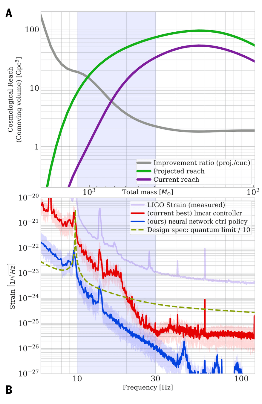
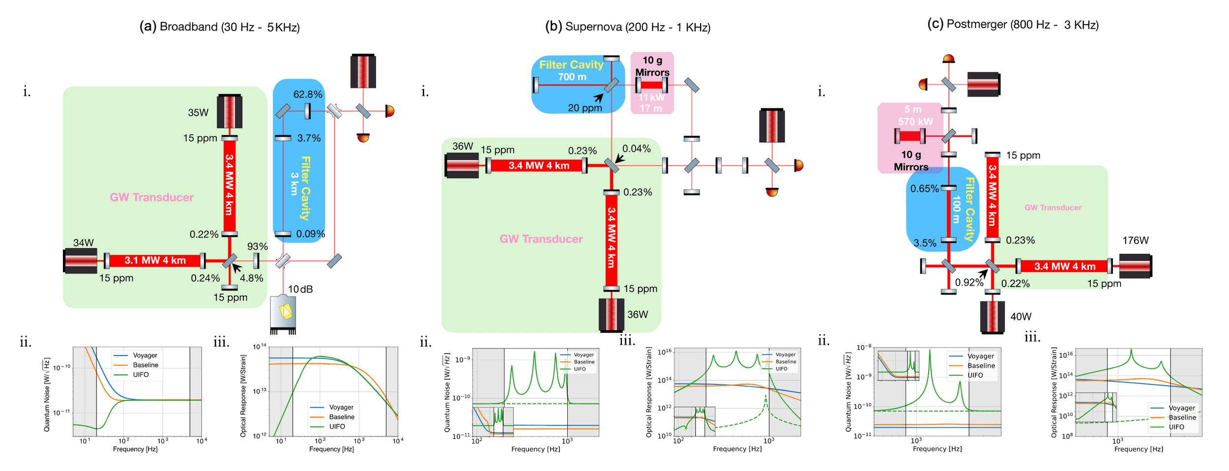
- Case 1 — AI-driven experiment design
- Experiment design as optimization
- The search object is no longer a parameter vector — it can be the experiment itself.
- Case 2 — Deep Loop Shaping for LIGO
- simulation-trained controller → real LIGO deployment
- The discovered object is a control policy, not a prediction.
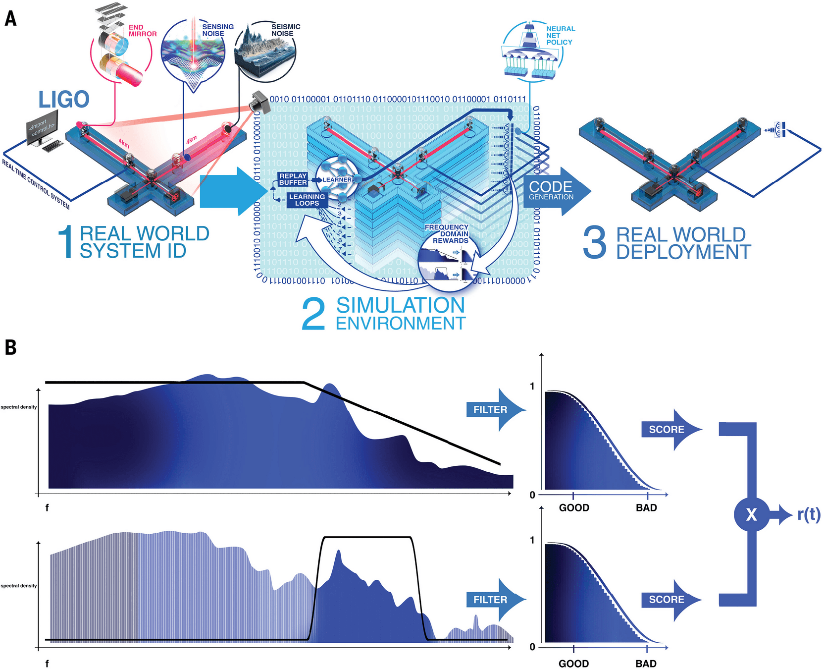
Once evaluation is executable, scientific design can enter a search loop.
Phys. Rev. X 15, 021012 (2025)
Buchli+, Science (2025)
AI Agent = LLM + Harness
The model decides what to do; the harness decides how it works.
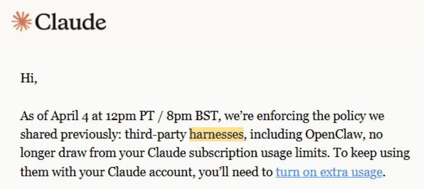
# Harness
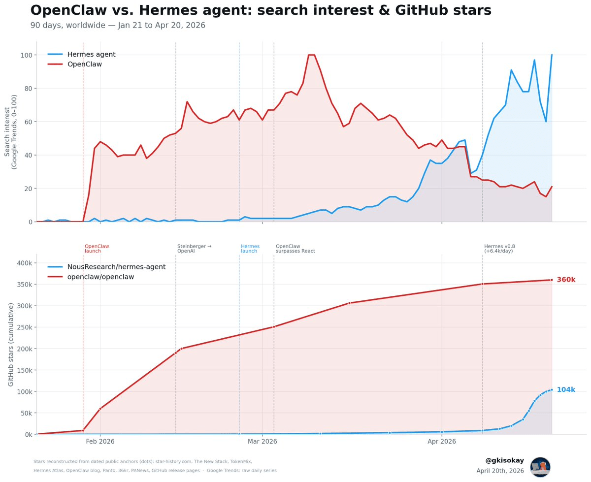
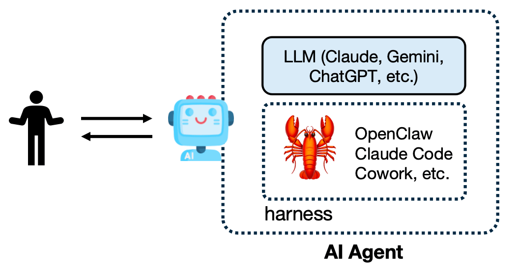
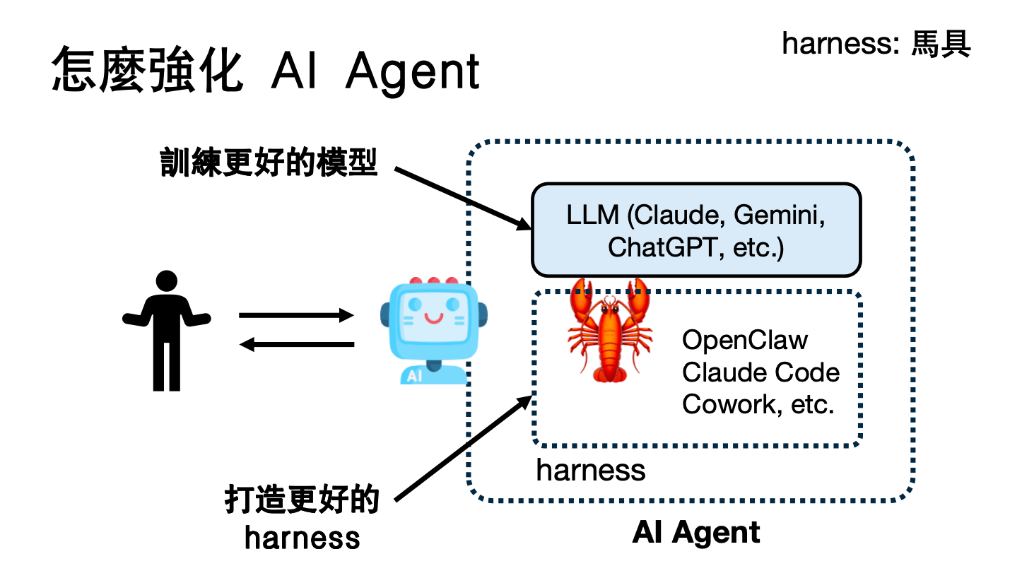
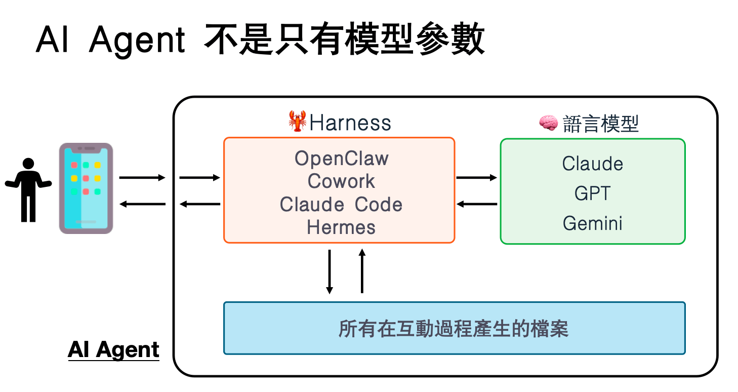
AI Agent is not just model parameters
训练更好的模型
Build a better Harness
Claude Code, Codex CLI, OpenClaw……
Much of today’s rapid progress comes from harness engineering, not only model scaling.
LLMs provide intelligence. Harnesses provide agency.
The model determines the upper limit of capability, while the Harness determines whether that capability can truly be realized.
The Interpolation Objection
# Discovery
Is deep learning really discovering — or mostly interpolating?
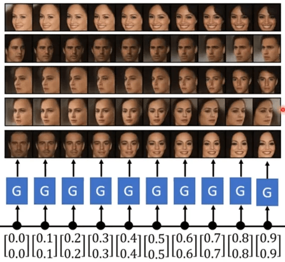
Much of deep learning’s empirical success can be understood as powerful interpolation over learned representations.
Deep Learning is Not As Impressive As you Think, It's Mere Interpolation (Source)
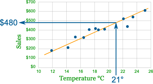
Linear Modeling
Interpolation in input space may be meaningless; interpolation in a learned latent space can be highly structured.
For example, the case of face morphing is a good one: pixel space linear interpolation and latent space interpolation are not the same thing. The real strength of deep models often lies in first organizing the data into a structured representation manifold, and then performing smooth generalization in that space.
The Interpolation Objection
# Discovery
Is deep learning really discovering — or mostly interpolating?
Much of deep learning’s empirical success can be understood as powerful interpolation over learned representations.
Representation Space Interpolation
Representation Space Interpolation
Deep Learning is Not As Impressive As you Think, It's Mere Interpolation (Source)
Interpolation in input space may be meaningless; interpolation in a learned latent space can be highly structured.
For example, the case of face morphing is a good one: pixel space linear interpolation and latent space interpolation are not the same thing. The real strength of deep models often lies in first organizing the data into a structured representation manifold, and then performing smooth generalization in that space.
Interpolation in the Right Space
# Discovery
The geometry of representation determines whether interpolation is meaningful.
Representation Space Interpolation
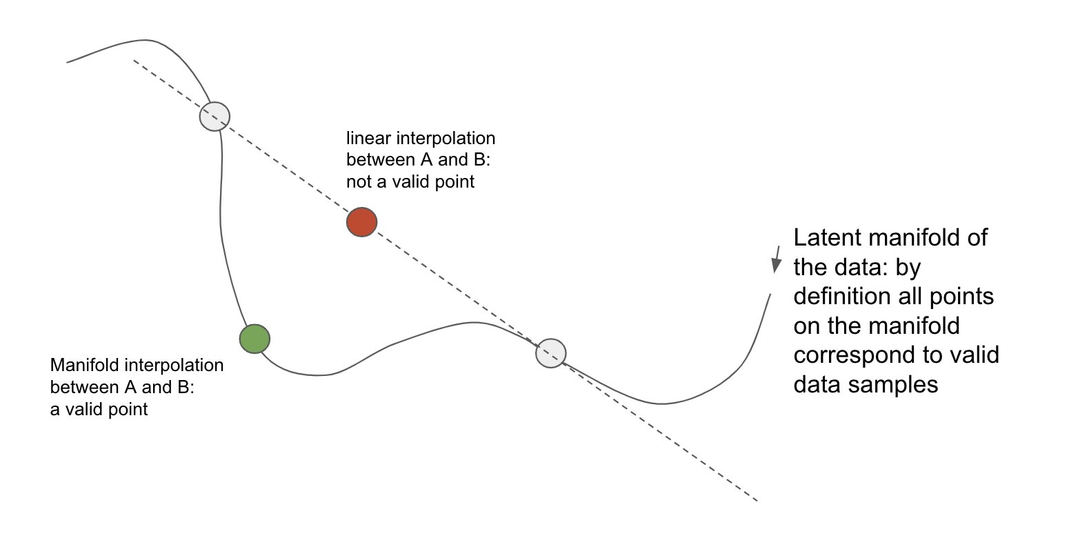
- Linear interpolation may leave the data manifold.
- A learned representation can bend the geometry.
- Interpolation along that geometry can remain semantically valid.
The power of deep learning often lies not in "arbitrary extrapolation," but in learning a representation that makes the originally complex data relationships smoother and easier to interpolate in this manifold space.
The trick is not to escape interpolation — it is to learn a space where interpolation becomes useful.
Deep Learning is Not As Impressive As you Think, It's Mere Interpolation (Source)
Why Does Data-Driven AI Generalize?
# Discovery
Generalization depends on how well data reveals the underlying representation space.
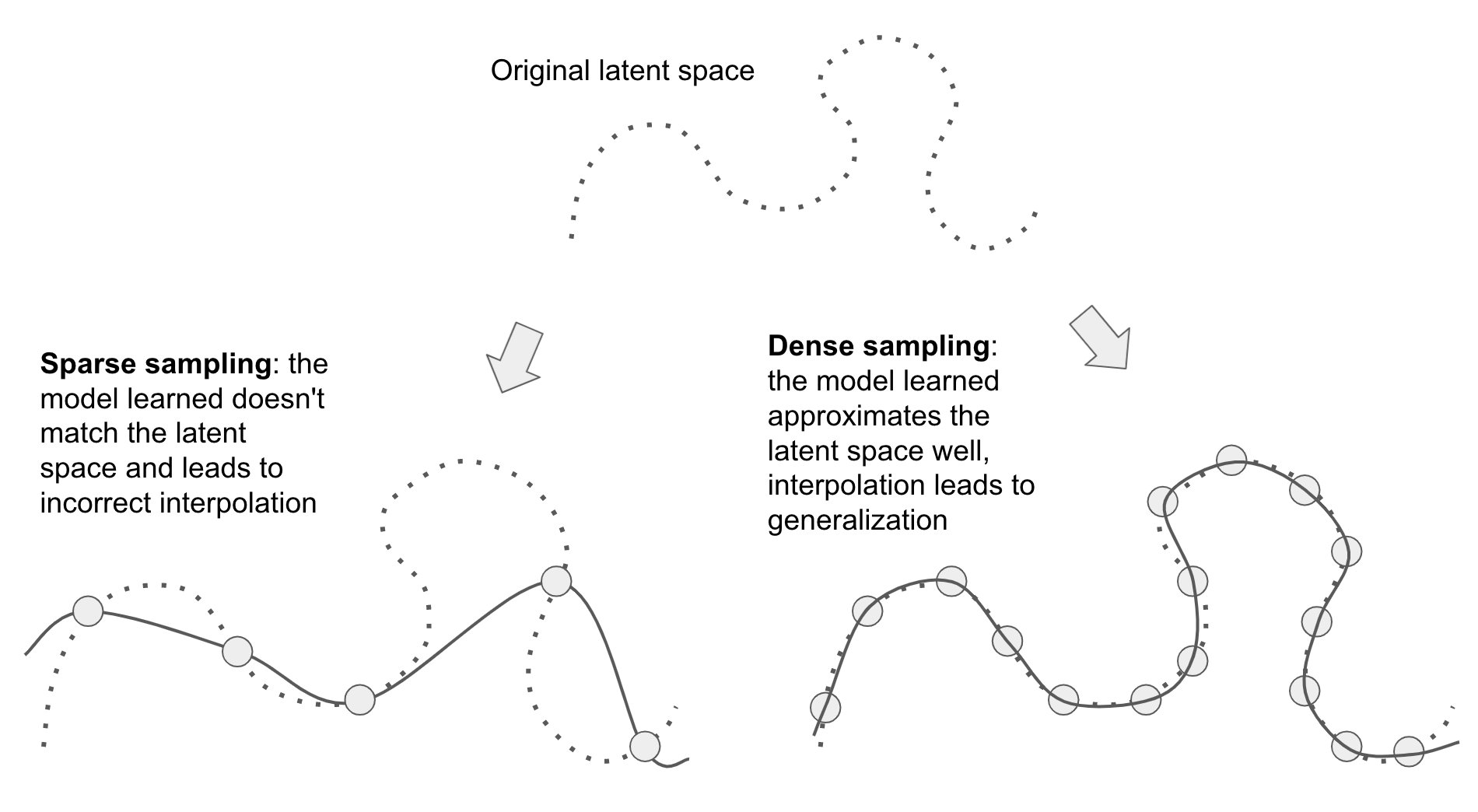
Generalization is not magic — it comes from structure shared between training and unseen data.
The reason AI can perform well on samples it has "never seen" does not mean it has truly encountered a completely unfamiliar world. Many times, although new samples have not appeared, they still fall within the same structure that the training data has already covered.
Deep Learning is Not As Impressive As you Think, It's Mere Interpolation (Source)
Underlying data manifold / latent structure
That is the "structure" of the true distribution of real data.
Sparse data → wrong geometry → poor generalization
When the training data is too sparse, the model can only guess this structure from a small number of samples, so the learned manifold may deviate from the true manifold.
Dense coverage → better representation → reliable interpolation
The more sufficient the data coverage, the easier it is for the model to learn a representation close to the true manifold, thus the generalization becomes more stable when doing interpolation near the covered structure.
LLMs appear highly general because their training distribution is extraordinarily broad.
GPT seems capable of answering a "previously unseen question," which does not necessarily mean it has done a far extrapolation in the strict mathematical sense; it is likely because the internet-scale training data has allowed the latent space to cover an extremely rich array of language, code, and knowledge structures.
So,
- Scaling can turn apparent extrapolation into interpolation in a richer learned space.
- The larger and richer the training distribution, the larger the region in which “interpolation” looks like intelligence.
- But science is often about finding what is not already well covered by the data. Where does novelty come from?
- Code
- Language
AI for Science: Search, Automated Verification, and Autonomy
- Shifting from game search to program-space search (AlphaEvolve, global exploration via local interpolation).
- Real-world application in mathematics (Terence Tao) and the power of low-cost, automated verification (e.g., Lean).
- The transition of AI for Science into global infrastructure and the roadmap toward autonomous scientists.
# Discovery
From Game Search to Algorithm Discovery
# Discovery
What changes is not only the model — but the object being searched.
Novelty Through Search
# Discovery
AlphaEvolve turns LLM proposals into verifiable algorithmic discoveries
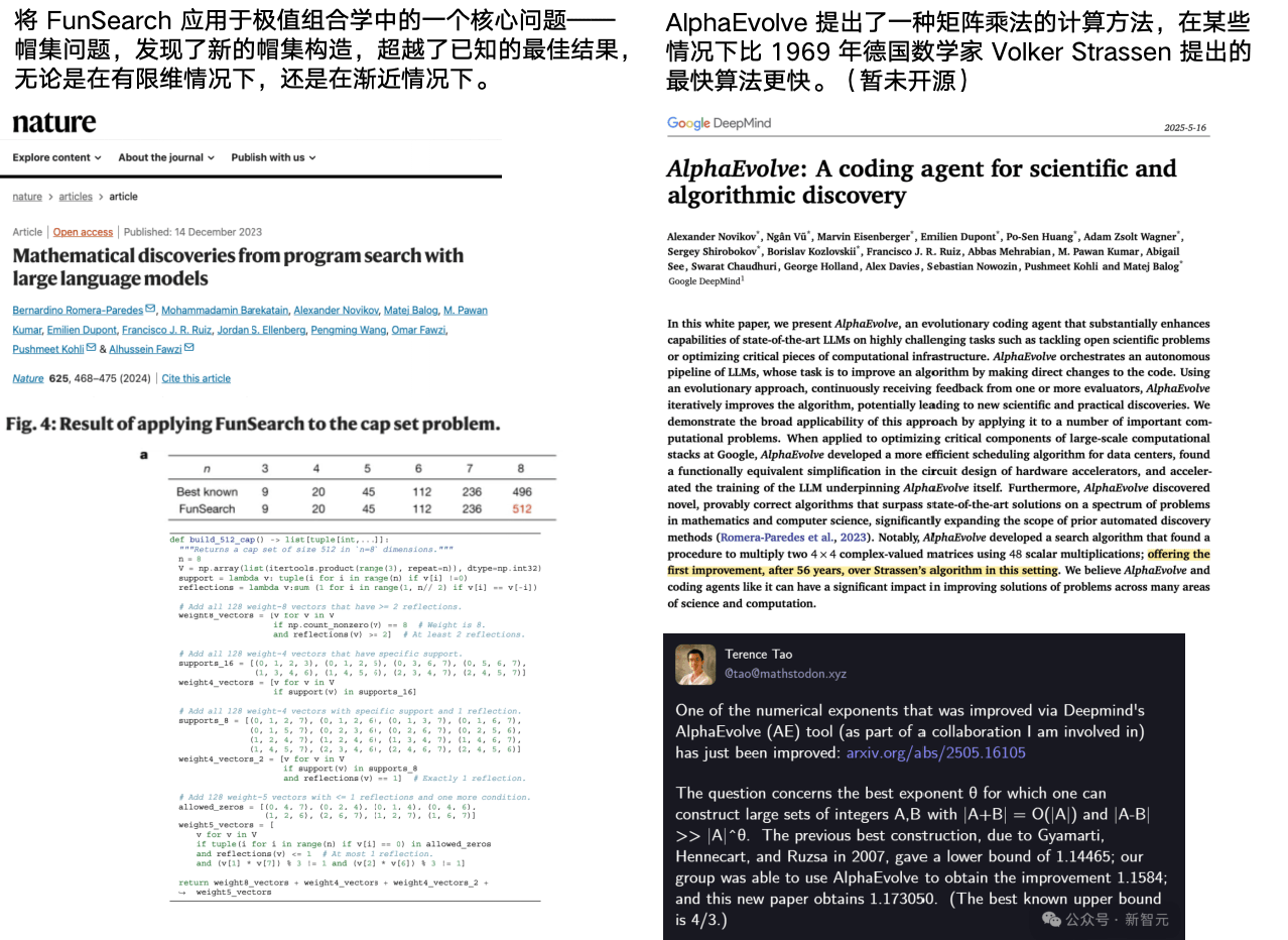
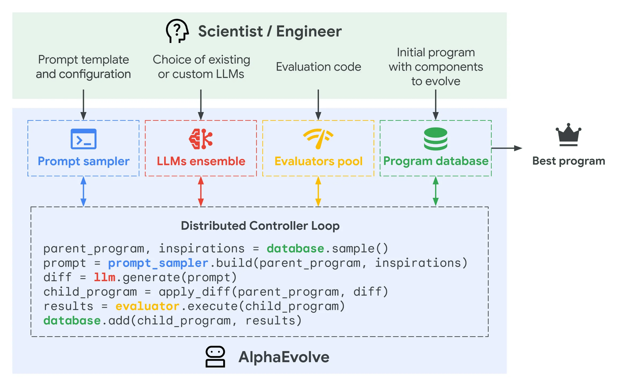
Tao’s perspective: AlphaEvolve is essentially trying to extremize complex high-dimensional functions when the good solutions are sparse and structured.
The model may interpolate locally; the system can still explore globally.
arXiv:2506.13131 [cs.AI]
AlphaEvolve in Mathematics
# Discovery
Terence Tao’s large-scale exploration across 67 mathematical problems
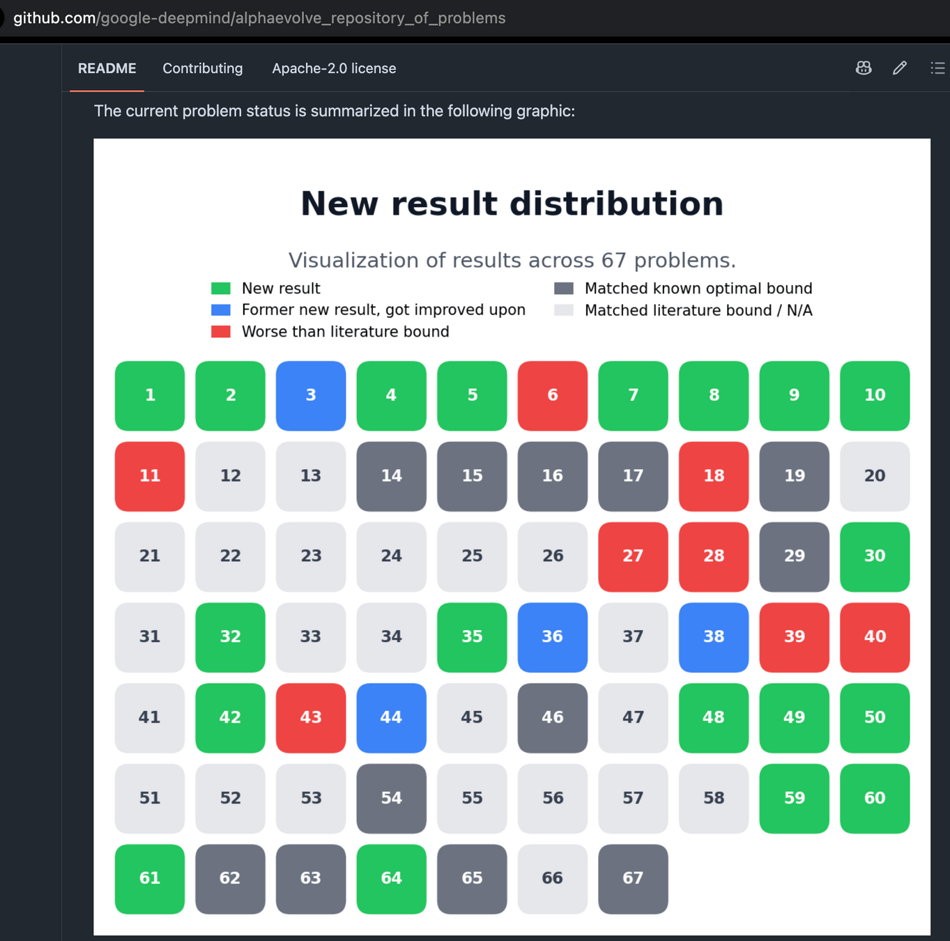
Tao mentioned sum-difference exponent:
\(1.14465 \rightarrow 1.1584 \rightarrow 1.173050\)
The intermediate increase comes from AlphaEvolve related explorations, which were further enhanced by new work.
Tao mentioned that in the exploration of arithmetic Kakeya / sum-difference exponent, after AlphaEvolve found candidate structures, these computational results further inspired him to obtain new rigorous theoretical results.
When Verification Is Cheap, Failure Can Be Cheap Too
# Discovery
Generate many formal proofs, reject most, keep the few that verify.

Most proposals can be wrong. LEAN simply rejects them.
Failure is acceptable because verification is exact and automated.
Today’s most scalable AI discovery systems are closer to automated search engines than autonomous scientists.
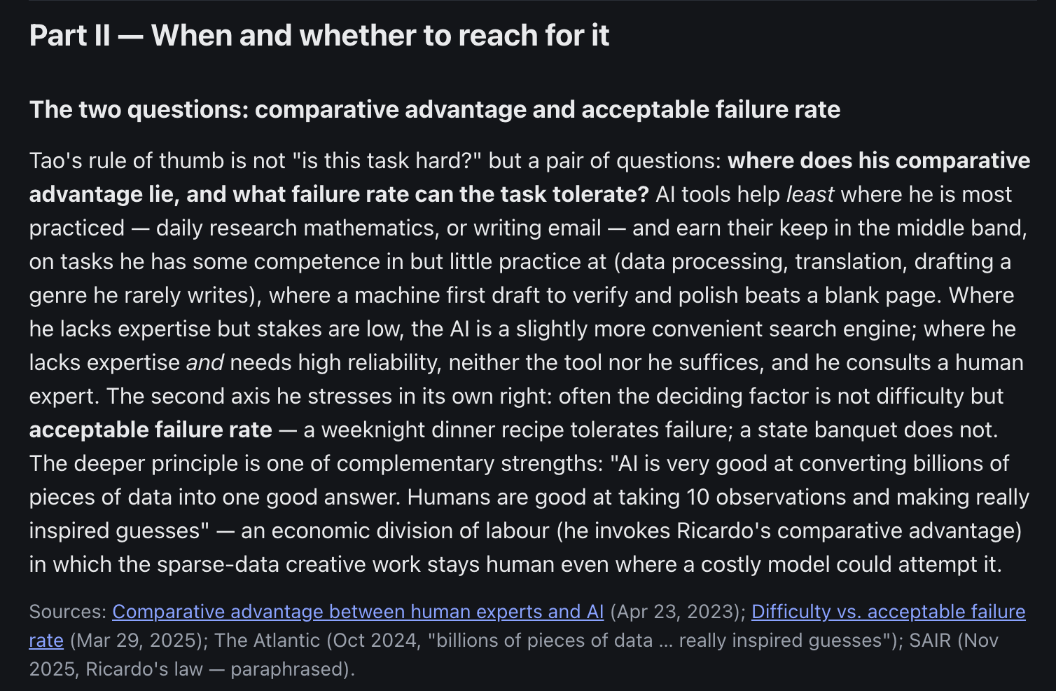

AI for Science Is Becoming Infrastructure
# Discovery
From isolated demos to national labs, frontier models, and closed-loop discovery platforms
In late 2025, the world embraced AI for Science!
- OpenAI CPO Kevin Weil announced OpenAI for Science, a platform using AI to enhance scientific discovery.
- On November 24, 2025, Trump signed the "Genesis Mission", an executive order focused on using AI to achieve scientific breakthroughs!
- DeepMind: sending "AI scientific collaborators" to national laboratories
- NVIDIA: transforming scientific issues into AI infrastructure challenges. AI for Science includes computing platforms, simulation systems, automated experiments, and engineering workflows as the foundation for Genesis.
- In August 2025, China's State Council released the "Opinions on Deepening the Implementation of the 'AI+' Action" (Guofa [2025] No. 11), stressing the need for a new AI-driven research paradigm to expedite major scientific discoveries.
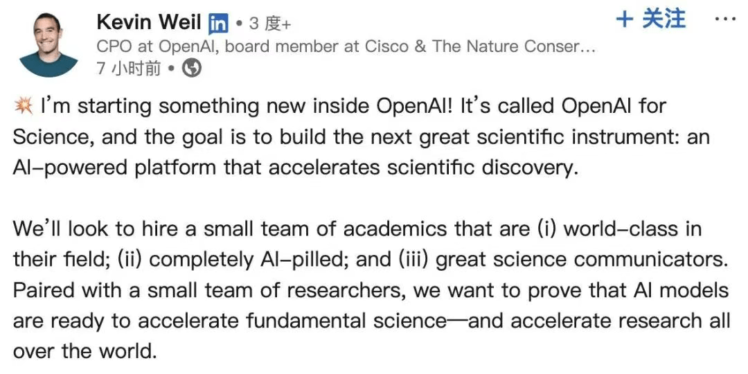
OpenAI plans to form a small team of top scholars who need to meet three criteria:
- Achieve world-class standards in their research fields;
- Deeply identify with the concept of artificial intelligence;
- Possess excellent scientific communication skills.

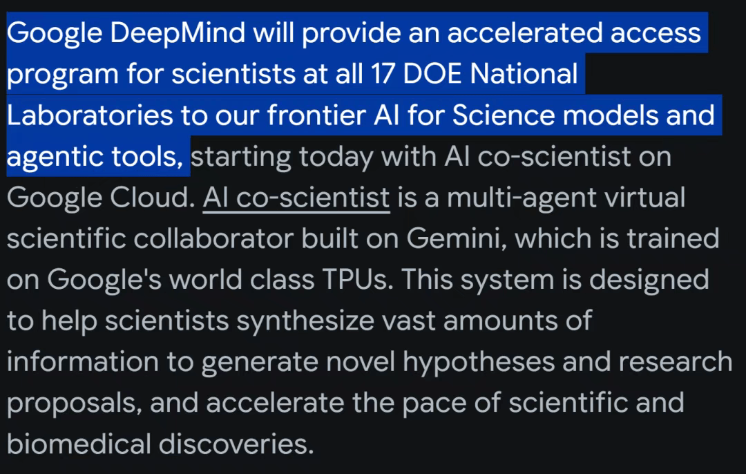
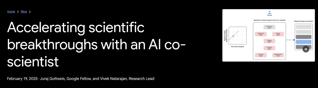
AI-driven scientific discoveries are moving from academic exploration to strategic competition.
From Scientific Assistant to Autonomous Scientist
# Discovery
As autonomy increases, LLMs move from evaluating science to collaborating on it—and eventually conducting it.
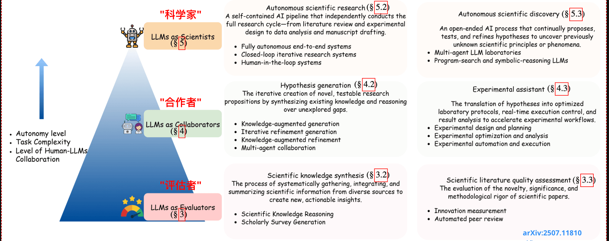
Content
-
What Is Machine Learning?
— The basics and why it matters -
Deep Learning: When Machines Start to See and Think
— From neural networks to powerful representations -
Gravitational Waves Meet Machine Learning
— How ML is reshaping data analysis in GW astronomy -
Natural Language Processing
— From transformer to three model families -
From Large Language Models to AI Agents
— Why are LLMs so powerful for automated scientific reasoning? -
Can AI Really Discover?
— From interpolation to search, verification, and science -
Harness Engineering for AI Agents
— How to utilize Claude Code, Codex, ...

A Strong LLM Can Still Fail as an Agent
# Harness
What changes when the same LLM is placed inside a different harness?
Your task is to fix the bug in `parser.py`.
Currently, the `extract_emails` function cannot correctly extract email addresses containing `-` or `_`, such as `test-user@domain.com`.
Please modify `parser.py` so that the tests in `verify.py` can pass completely.
You are an AI Agent. You can interact with the environment by writing code blocks.
If you write a ```bash\n...\n``` block, the system will execute it and return the output.
If you write a ```python\n...\n``` block, the system will execute it and return the output.
To finish the task, output 'DONE'.
Provided tool :
Not provided "parser.py"
...... I'll write one myself
parser.py
def extract_emails(text): ……
# Example test cases to verify the fix
test_string_1 = ……
DONE

What Was Missing?
# Harness
What changes when the same LLM is placed inside a different harness?
[CONTEXT]
You are running in a Linux environment (Google Colab). You need to find and modify the correct files to achieve the goal.

[INSTRUCTIONS]
1. Before modifying anything, you MUST inspect the current working directory, system environment, and file tree.
2. List all potentially relevant files.
3. Do not blindly modify files without looking at their contents first.


[DONE-WHEN]
You are done ONLY when the specific success criteria mentioned in the task are met, and the expected artifacts exist.
Current Environment
How it works
How to consider it complete
If: add some extra prompts
Now It Behaves Like an Agent
# Harness
What changes when the same LLM is placed inside a different harness?
…
First, I will list the files.
```bash
ls -R
```
--- Bash Execution ---
parser.py
verify.py…
I will now display the content of `parser.py`.
```bash
cat parser.py
```--- Bash Execution ---
import re
def extract_emails(text):
……```bash
cat <<EOF > parser.py
def extract_emails(text):
……
EOF
```--- Bash Execution ---…
I will execute `verify.py`.
```bash
python verify.py
```--- Bash Execution ---
VERIFY_SUCCESSThe intelligence may be in the model — but the competence emerges from the loop.
If: add some extra prompts
Why the Harness Matters: The Core to Agent Performance

# Harness
- LLMs
- Harnesses
- Interactive Discovery
Harness Engineering Is Becoming a Discipline
# Harness

As models become stronger, harness engineering becomes the new bottleneck.
OpenAI officially introduces “Harness Engineering”. (2026.02.11)
The focus shifts from prompts to reliable systems. (2026.03.24)
Harness: equipment for controlling a horse
Anthropic: Harness engineering (2025.11.26)
From Prompt Engineering to Harness Engineering
# Harness
Prompt → Context → Harness → Agent System
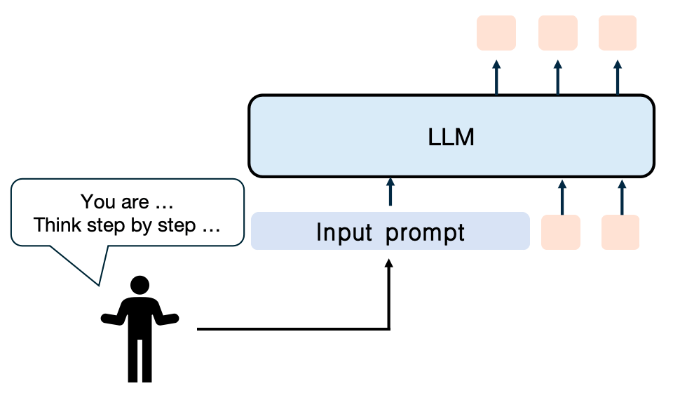
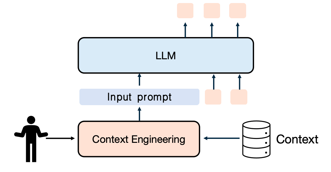
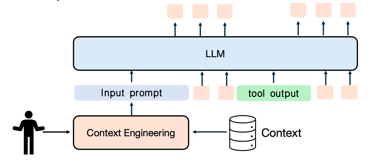
Engineering has shifted from prompts to systems.
Prompt Engineering(2023)
Everything is encoded into a single prompt.
- Static
- One-shot
- Prompt-centric
Context Engineering(2024–2025)
Context, not the user, increasingly writes the prompt.
- RAG
- Memory
- File system
- History
Harness Engineering(2025~)
The prompt becomes only one component of a complete execution system.
• Tool execution
• Context management
• Memory & State
• Planning & Reflection
• Verification & Recovery
Harness can be optimized
# Harness
AGENTS.md and CLAUDE.md are examples of reusable harness specifications.
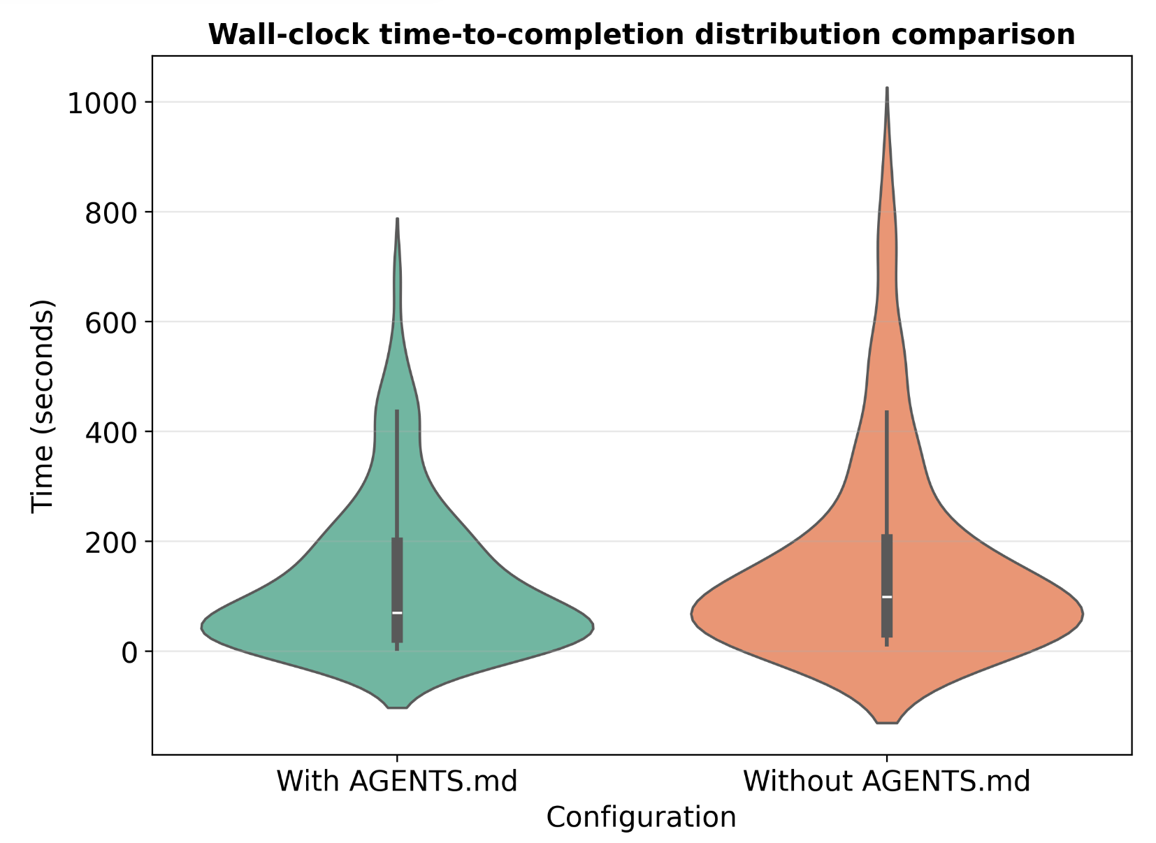
arXiv:2601.20404 [cs.SE]
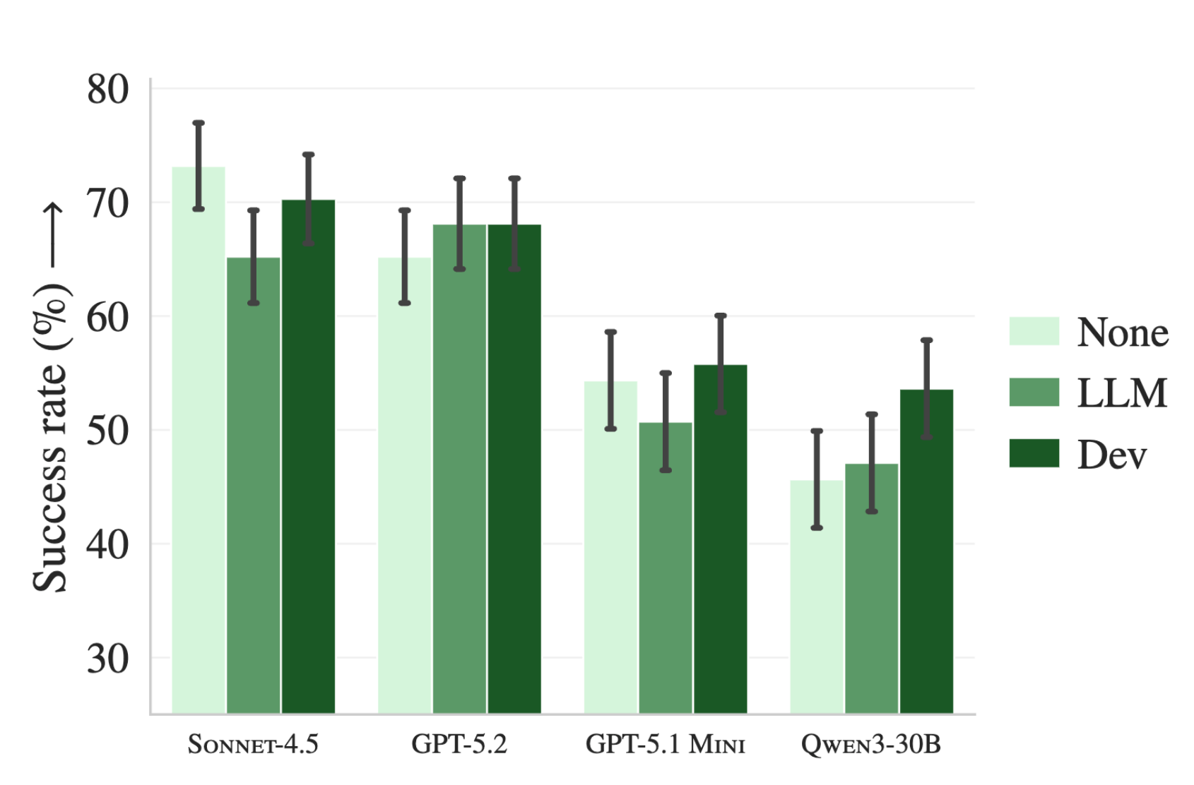
arXiv:2602.11988 [cs.SE], https://agents.md/
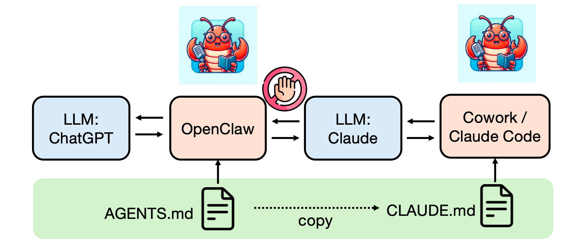
Better harnesses complete tasks faster.
Better harnesses improve success rates.
- Harness has a more significant improvement for small LLMs
- AGENT.md/CLAUDE.md should not be too long
- LLMs favor early and recent tokens in your prompt.
- ...
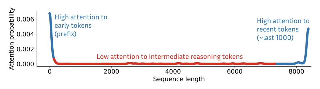
| arXiv:2608.26070 [cs.CL] |
The first and last few tokens receive most attention during reasoning with full attention.
Tools should be designed for AI agents, not humans.
# Harness
Better tools reduce reasoning and interaction overhead.
Tools designed for humans may not necessarily be suitable for AI Agents.
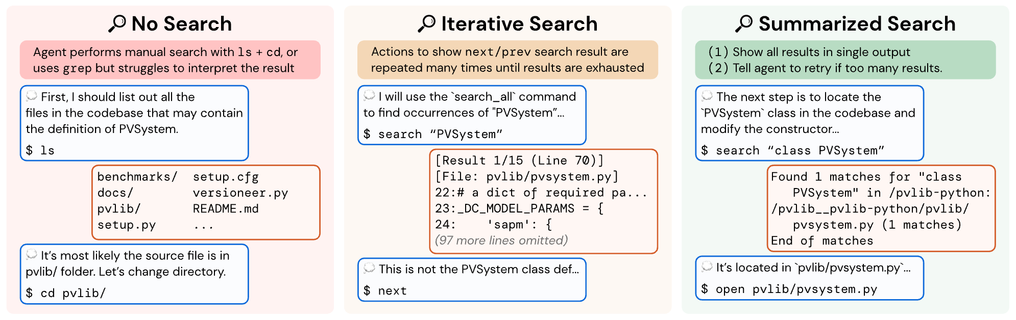
SWE‑agent (Agent-Computer Interface, ACI) (NeurIPS 2024)
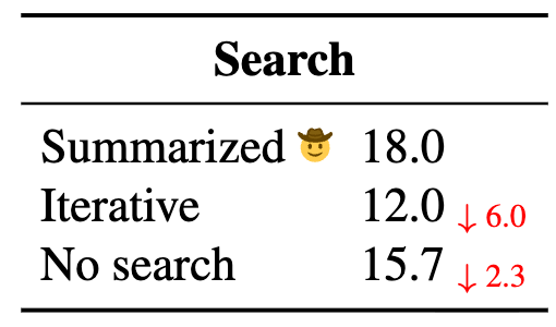
Tools should be designed for AI agents, not humans.
# Harness
Better tools reduce reasoning and interaction overhead.
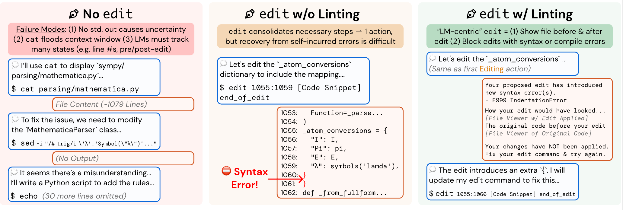
SWE‑agent (Agent-Computer Interface, ACI) (NeurIPS 2024)
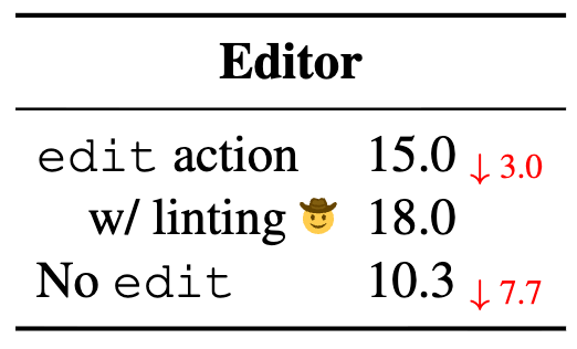
Tools designed for humans may not necessarily be suitable for AI Agents.
Tools should be designed for AI agents, not humans.
# Harness
Better tools reduce reasoning and interaction overhead.
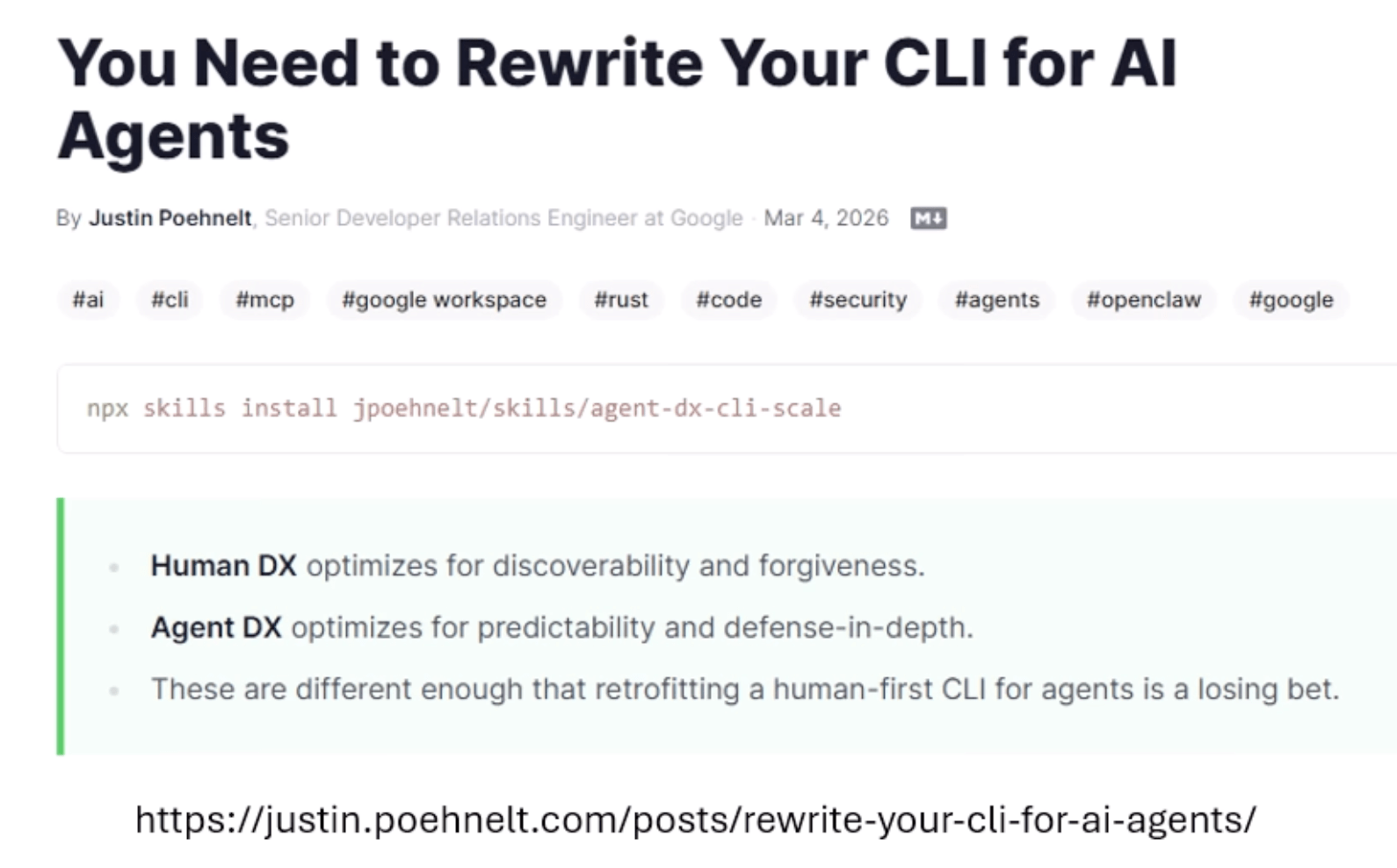
Managing Long-Horizon Agent Workflows
# Harness
Long-running agents cannot simply keep appending history forever.
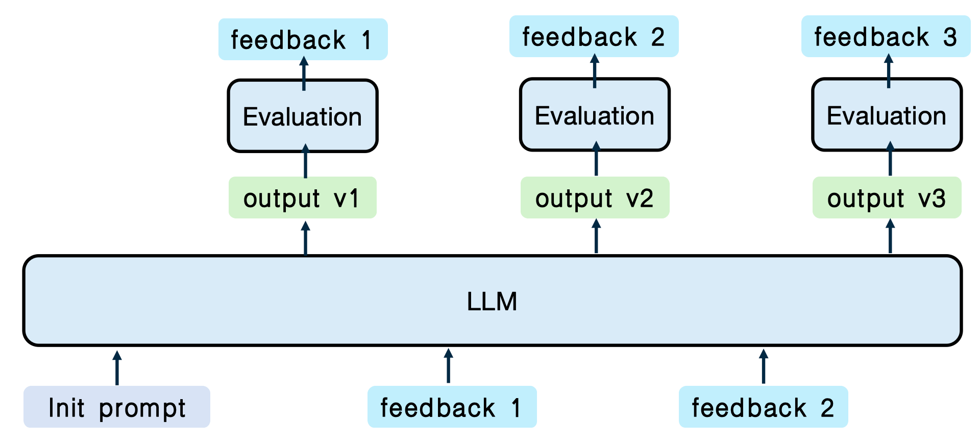
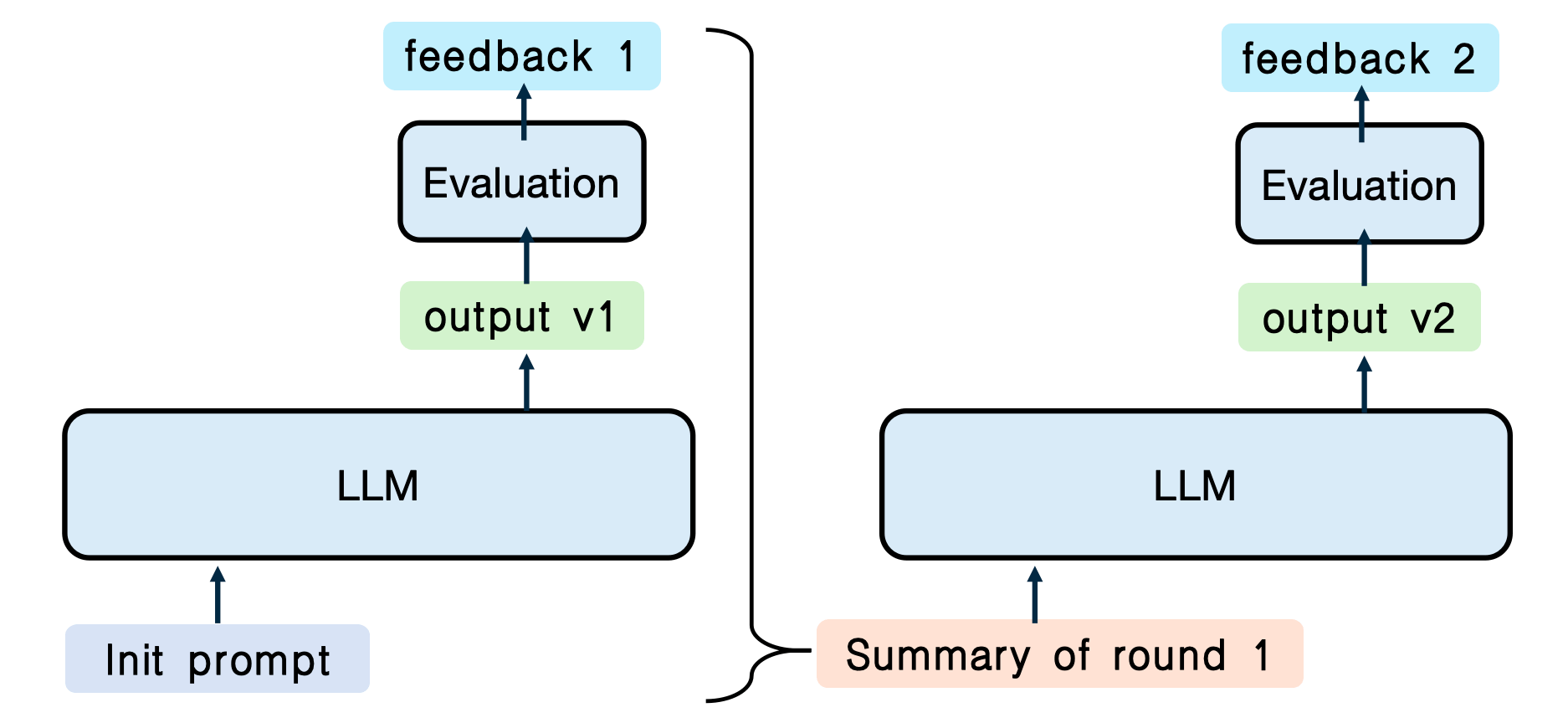
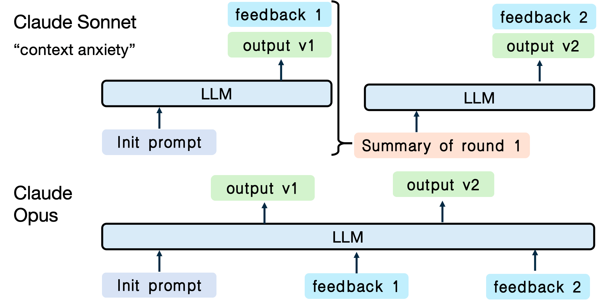
Context grows continuously.
Summaries replace raw interaction history.
Good harnesses preserve information, not tokens.
Recommended Reading
Ralph
— Standard workflow for AI coding agents
ghuntley.com/ralph
Loop
— Reliable agent execution loops
ghuntley.com/loop
Harnesses Can Also Learn
# Harness
Beyond optimizing LLMs, we can optimize the harness itself.
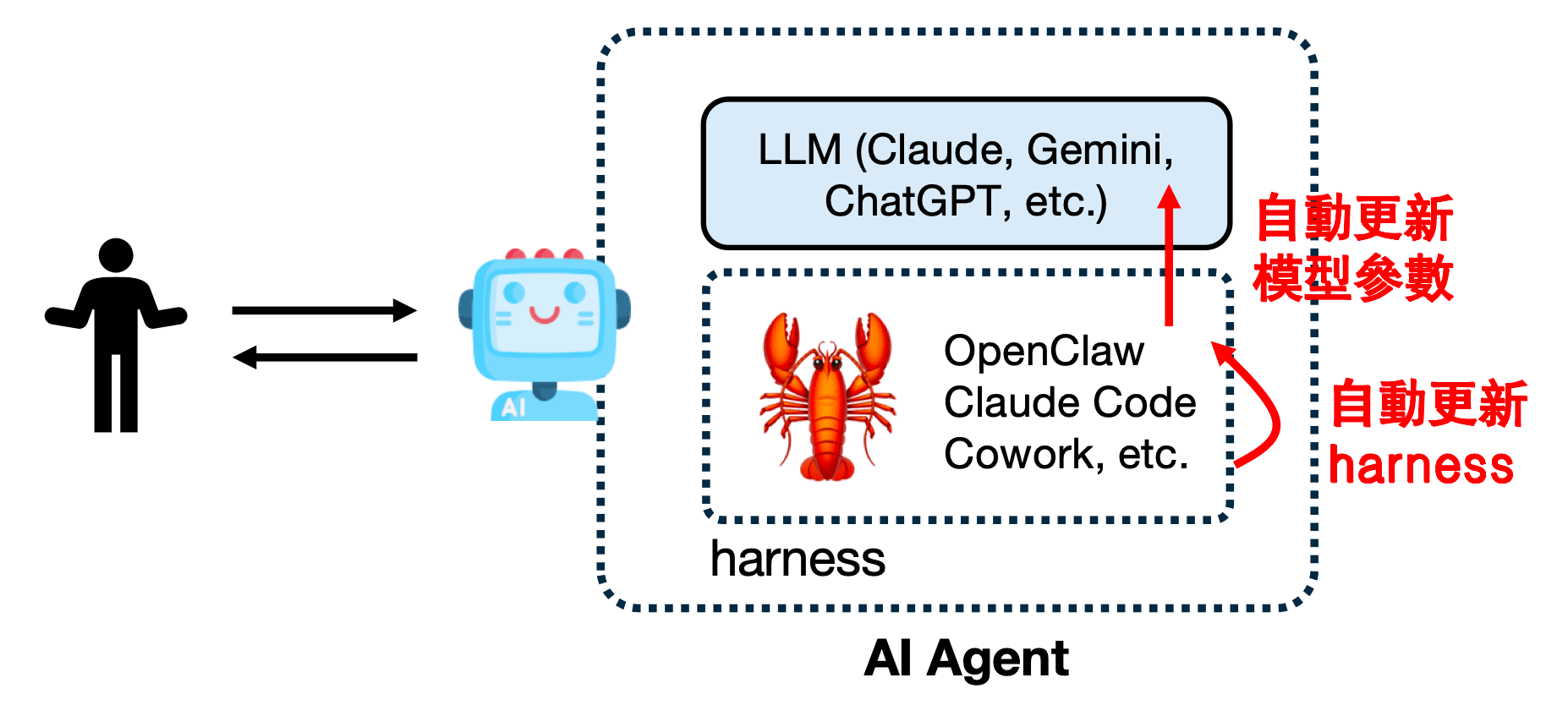
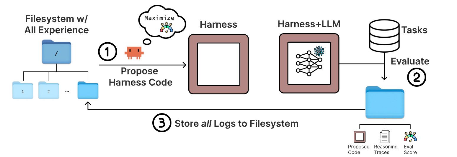
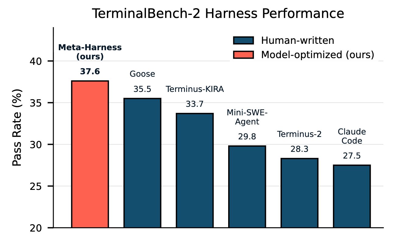
Meta-Harness. arXiv:2603.28052 [cs.AI]
The optimization target is shifting from models to complete agent systems.
Omitted
Automatically update model parameters
Automatically update harness
Agent Engineering in Practice

# Harness
- model selection
- benchmark trade-offs
- harness toolchains
- human-in-the-loop inquiry
Building Your Own AI Agent
# Harness
Choosing the right LLM and the right harness.
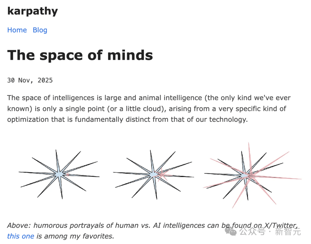
Do not believe in only one "best model".
- I basically switch between Claude, GPT, Gemini, and Deepseek almost every day now.
- Not because one is absolutely stronger, but because their "ways of thinking" are different.
Switch models without changing workflows.
Building Your Own AI Agent
# Harness
Choosing the right LLM and the right harness.
# Harness
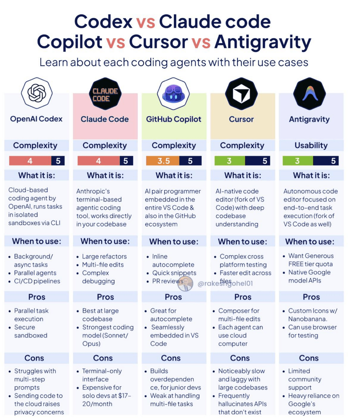
Building Your Own AI Agent
Choosing the right LLM and the right harness.


Question Engineering for Human-in-the-Loop Discovery
Navigating the Space of Ideas
# Harness
I want to conduct an experiment. You can ask me any question you like, and I will respond as truthfully and completely as possible. Based on my answers, you can then proceed to ask the next question or present options for me to choose from. We will continue this back-and-forth until we unearth the thoughts deep within me—discovering fallacies, limitations, potentials, areas for improvement, or anything lurking in my subconscious.The most valuable output of an AI agent is sometimes not an answer, but the next question.
Your starting area
Points of AI Association
Your target,
which remains unseen
All known knowledge and collected data
Only assume valid points on the line.
# END
This slides: https://slides.com/iphysresearch/2026aug_fqcp
hewang@ucas.ac.cn
for _ in range(num_of_audiences):
    print('Thank you for your attention! 🙏')
# End
for _ in range(num_of_audiences):
    print('Thank you for your attention! 🙏')
This slides: https://slides.com/iphysresearch/2026aug_fqcp
hewang@ucas.ac.cn

for _ in range(num_of_audiences):
    print('Thank you for your attention! 🙏')
Thank You & Q&A
# Conclusion & Q&A
• AI for Science: Automated reasoning, verification & LLM agents
• Harness Engineering: Building robust workflows for scientific discovery