EMRI Search and Inference within the LISA Global Fit — Part II
National University of Singapore · 14 July 2026
ICTP-AP, University of Chinese Academy of Sciences (UCAS)
Taiji Laboratory for Gravitational Wave Universe, UCAS
In collaboration with Dingkai Zhang, South China Normal University
(in prep.)
He Wang
One learned foreground model for calibrated noise reconstruction and foreground-aware source inference
Learning a Robust Foreground Models for Multi-Source GW Inference






Abstract
- Space-based gravitational-wave data analysis will involve strongly overlapping signals and unresolved astrophysical foregrounds, which can bias the characterization of instrumental noise and affect the validation and inference of weaker scientific targets, including EMRI-like sources.
- In this talk, I will discuss how robust data-driven models can be learned from simulated multi-source data to characterize effective noise and foreground-induced distortions. The goal is to improve the reliability of downstream analyses for specific scientific targets in complex scenarios of signal confusion.
- I will also discuss how such models can be incorporated into global-fit workflows, where noise estimation, foreground subtraction, and source validation are treated as coupled components of a sequential inference problem.
才翻到上面看到有人现场拍照 [破涕为笑],随手分享一下
- 我最近常用的PPT英语字体是 Economica,是一个风格比较现代的无衬线字体:https://fonts.google.com/specimen/Economica
- 但用这个字体显得好看,牺牲了一点儿清晰度,有需要的时候还是会回归Helvetica Neue
- 衬线字体我喜欢用 Arno Pro: https://fonts.adobe.com/fonts/arno
- 中文字体已经锁死了喜鹊宋或者木叶(收费字体)
- 颜色一般从MetBrewer里面挑,但并没有特别注意配色:https://github.com/BlakeRMills/MetBrewer
- 今天刚和邵老师说,可能是中年危机的一种表现,就现在越来越喜欢五颜六色的东西。。。也体现在了PPT上。这个完全见仁见智。
- 如果有人对这种PPT感兴趣,我把一个7月份会议的短PPT分享在这供参考:https://www.dropbox.com/scl/fi/duez2bpbcck4ogtn98sw6/songhuang_sesto_20250707.key?rlkey=g18rnjym1hpzke3jxcj5y6ezh&st=ot5xu2w8&dl=0
- 我自己现在习惯的PPT排版的风格只适合分steps展示,不能一次都show全。我自己开始使用这个风格是上课以后,需要满足PPT好看,能吸引注意力,但同时信息量够足,学生可以拿来复习。暂时觉得还好,但过两年可能还是会学着做简单一点儿。
- 用字体大小和颜色来highlight关键词是最简单粗暴、最俗的引导视线的方法,属于广告里早就用烂了的。其实有更好的设计语言,但不会。。。
- PPT风格纯属个人审美兴趣,和报告水平,更和报告内容好坏无关。
The millihertz data stream is signal-dominated, not noise-dominated.
Tens of millions of Galactic binaries overwhelm the instrumental floor across the band where many high-value sources live.
One-year Taiji simulation
- \(\sim 4.5\times10^7\) Galactic binaries
- numerical Taiji orbit
- unequal-arm TDI-2.0
- frequency-domain \(A/E\) channels
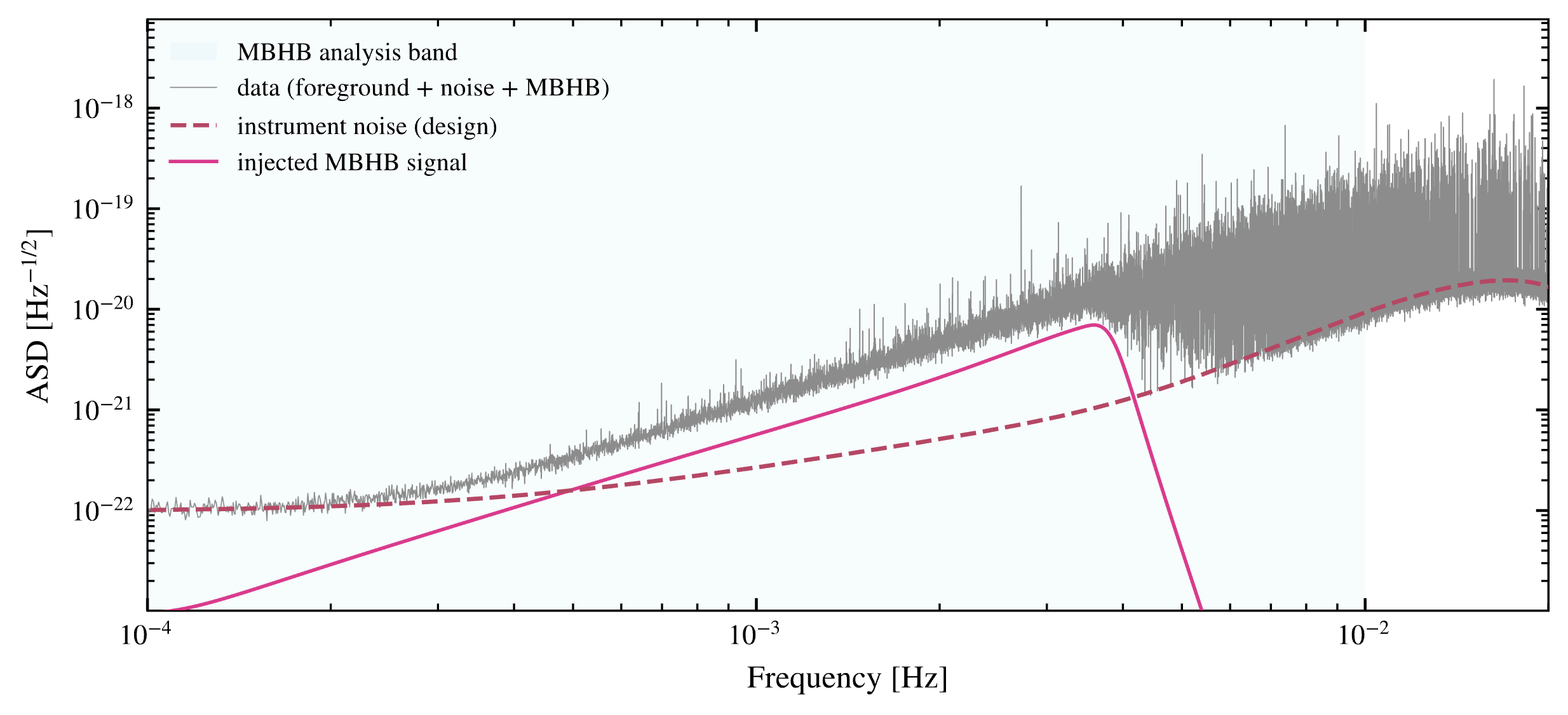
Why is this difficult?
- Confusion dominates: \(\sim0.3\)–\(10\) mHz
- No signal-free frequency region
-
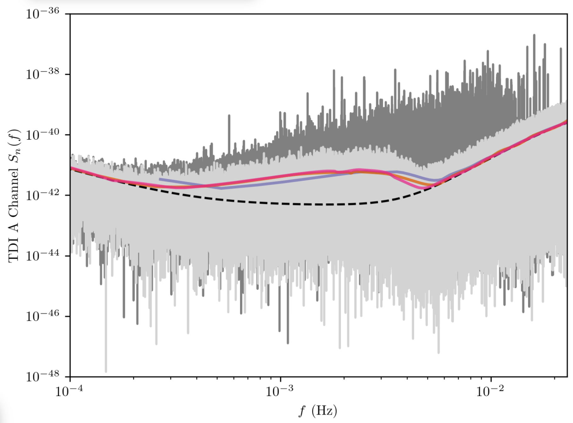
Foreground and instrumental noise cannot be separated directly
There is no clean off-source measurement of the instrumental PSD.
How can we estimate the instrumental PSD
when no frequency region contains only noise?
Credit: Dingkai Zhang

\(\widehat S_{\rm res}(f)\neq S_{\rm inst}(f)\)
- foreground power contaminates the residual periodogram
- the inferred PSD is systematically distorted
- frequency-dependent likelihood weights become incorrect
Galactic foreground biases instrumental PSD estimation.
Signal confusion creates two coupled inference failures
Foreground contamination biases the noise model and leaves structured residuals that degrade downstream source inference.
A contaminated residual means both a distorted PSD and a misspecified source likelihood.
Noise characterization fails
\(r(f;\theta)=d(f)-h(f;\theta)=g_{\rm GB}(f)+n(f)\)
\(r(f;\theta)\not\sim\mathcal N\!\left(0,S_{\rm inst}(f)\right)\)
- the residual contains structured foreground power
- the assumed Gaussian-noise likelihood is misspecified
- posteriors can broaden, shift, or become overconfident
Target-source model is misspecified
Littenberg & Cornish (2023)
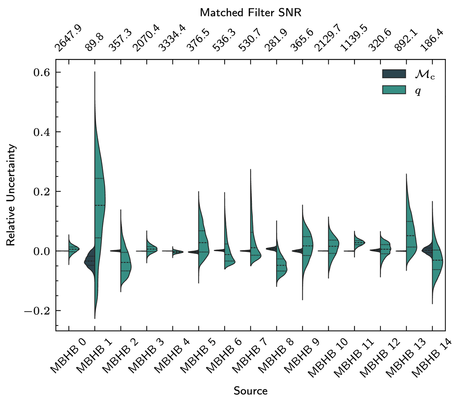
Foreground residuals degrade source inference.
Deng, Babak, and Marsat (2025)
For noise calibration and target inference, the aggregate foreground may be more important than the identity of every source.
The global fit solves the problem—but at a price
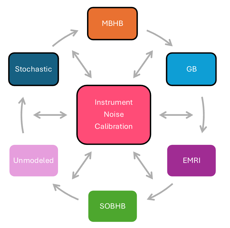
A global fit resolves the coupling in principle, but does so by explicitly modeling individual sources.
Scientific Question
Do we need the identity of every Galactic binary
to infer the instrumental noise
or validate one target source?
Katz, Karnesis, Korsakova, Gair, and Stergioulas (2025)
What the global fit provides
- individual source catalogs
- physical noise posterior
- joint Bayesian consistency
- interpretable residuals
What it costs
- trans-dimensional sampling
- repeated waveform generation
- blocked iterative convergence
- computational cost scales with source number
One learned foreground model, three uses.
- Learn
population-conditioned training
\(\rightarrow\) frequency-bin–shared foreground network - Characterize
foreground-subtracted residual
\(\rightarrow\) unbiased \(A_{\rm acc}, A_{\rm oms}\) + bounded distortion - Deploy in-loop
cached subtraction inside MBHB MCMC
\(\rightarrow\) oracle-level posteriors
Our key design choice: learn the aggregate foreground
The network predicts the total Galactic foreground, which is then reused for noise characterization and source inference.
左侧图
四个块:
- GB catalog
- Instrument noise
- MBHB / EMRI / other targets
- Residual validation
箭头循环:
GB subtraction
$\rightarrow$ noise update
$\rightarrow$ target-source inference
$\rightarrow$ residual
$\rightarrow$ GB update
Katz, Karnesis, Korsakova, Gair, and Stergioulas (2025)
(adapted)
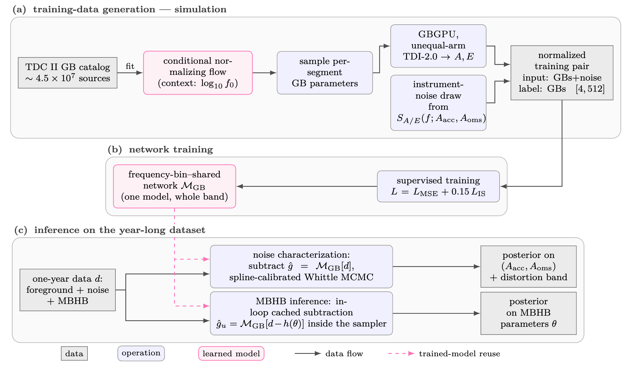
Aggregate
Foreground
learned by
Pipeline overview
No catalog in, no catalog out.
Aggregate foreground is the prediction target.
A one-year Taiji signal-confusion dataset
The testbed is a one-year Taiji TDC II realization
We test the idea on an orbit-accurate, unequal-arm Taiji signal-confusion dataset.
\(T_{\rm obs}=3.154\times10^7\) s
\(\Delta t=15\) s
\(\Delta f=1/T_{\rm obs}\simeq3.17\times10^{-8}\) Hz
Observation
\(A_{\rm acc}=3\times10^{-15}\)
\(A_{\rm oms}=8\times10^{-12}\)
Instrument noise
TDC II Galactic-binary catalog
\(\sim4.5\times10^7\) GBs
Galactic Foreground
no resolvable/unresolved split
GBGPU waveform generation
numerical Taiji orbit
Detector response
TDI-2.0 unequal-arm \(X,Y,Z\)
\(A=(Z-X)/\sqrt{2}\)
\(E=(X-2Y+Z)/\sqrt{6}\)
The injected noise and the analytic inference model belong to the same unequal-arm PSD family.
Open datasets and selected analysis tools: https://github.com/TriangleDataCenter
Population-conditioned simulation
The network learns a population—not a catalog
Every training sample is a new foreground realization, preventing catalog memorization.
TDC II catalog
\(\rightarrow\) sample source parameters and counts
\(\rightarrow\) GBGPU + Taiji response
\(\rightarrow\) TDI-2.0 A/E segment
Conditional normalizing flow:
- Target: \(p(\theta_{\rm GB}\mid \log_{10}f)\)
Key choices:
- full catalog, no SNR split
No realization is ever repeated.
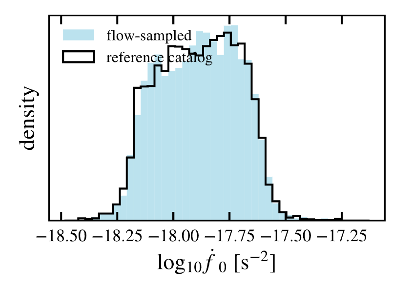
Population validation near 1 mHz
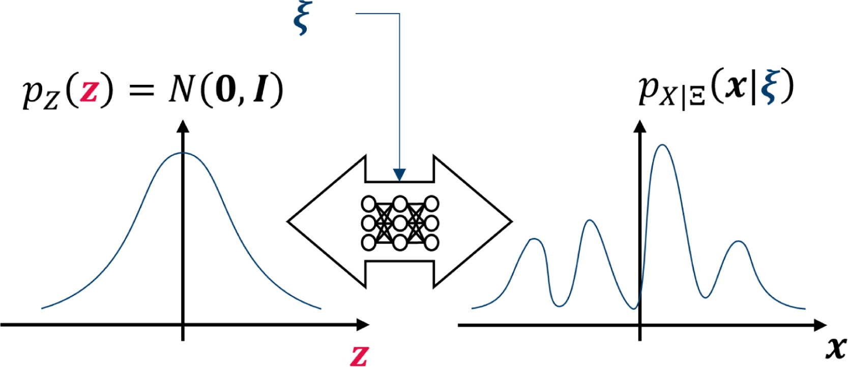
Conditional normalizing flow
One frequency-bin–shared network
One shared network covers the full analysis band
Local spectral morphology is sufficiently universal for one shared network to operate across the entire band.
Input representation
\(x\in\mathbb{R}^{4\times512}\)
Local 512-bin window in A/E channels
Why one shared network?
- local morphology is translation-invariant
- dense and sparse regions share the same representation
- frequency enters only through conditioning
Sliding inference
- overlapping windows
- crop borders
- stitch predictions
Key choices:
- random source counts: \(N_{\rm ref}(f)\pm2\sqrt{N_{\rm ref}(f)}\)
- bleed padding near segment edges
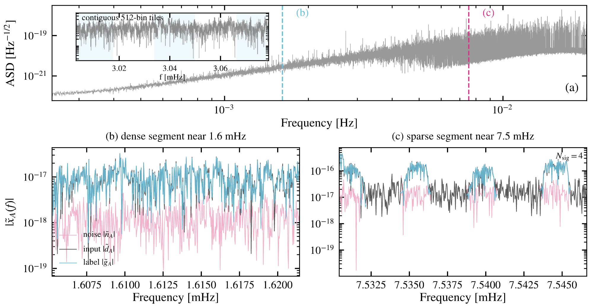
Shared morphology enables a shared network.
The architecture is simple; the training objective makes the residual usable
The loss is designed for the downstream likelihood, not just foreground reconstruction.
Calibrate the residual, not just the prediction.
Downstream-aware objective
\(\mathcal{L} = \mathcal{L}_{\rm MSE} + \lambda\mathcal L_{\rm IS},\qquad\lambda=0.15\)
\(\mathcal{L}_{\rm IS}=\frac{1}{M}\sum_{c,j}\left[\frac{R_{c,j}}{T_{c,j}}-\ln\frac{R_{c,j}}{T_{c,j}}-1\right]\)
where
- \(R_{c,j}=\left\langle |d_c-\hat g_c|^2\right\rangle_j\) is block-averaged residual power
- \(T_{c,j}=\left\langle |n_c|^2\right\rangle_j\) is block-averaged injected noise power
- \(j\): eight coarse 64-bin sub-bands
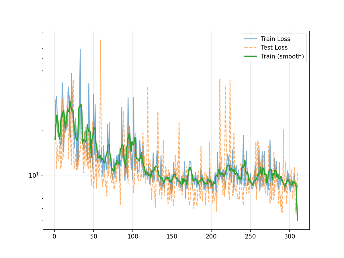
Loss landscape
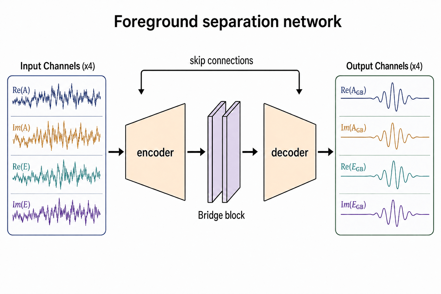
A constant-length 1D convolutional encoder–decoder
Model and training at a glance
The architecture is deliberately simple; the robustness comes from data generation and calibration
Input: \([B,4,512]\)
Output: predicted GB foreground
Architecture:
- Conv1D, \(k=31\)
- BatchNorm + ReLU
- encoder–decoder with skip concatenations
- \(\sim5.2\times10^8\) parameters
Training:
- Adam, learning rate \(10^{-3}\)
- batch size 128
- bfloat16 mixed precision
- \(\gtrsim2.4\times10^4\) optimizer steps
网络结构图
No attention, no catalog lookup, no per-band retraining.
One shared network generalizes across the full Galactic foreground
No retraining. No per-band tuning. One model everywhere.
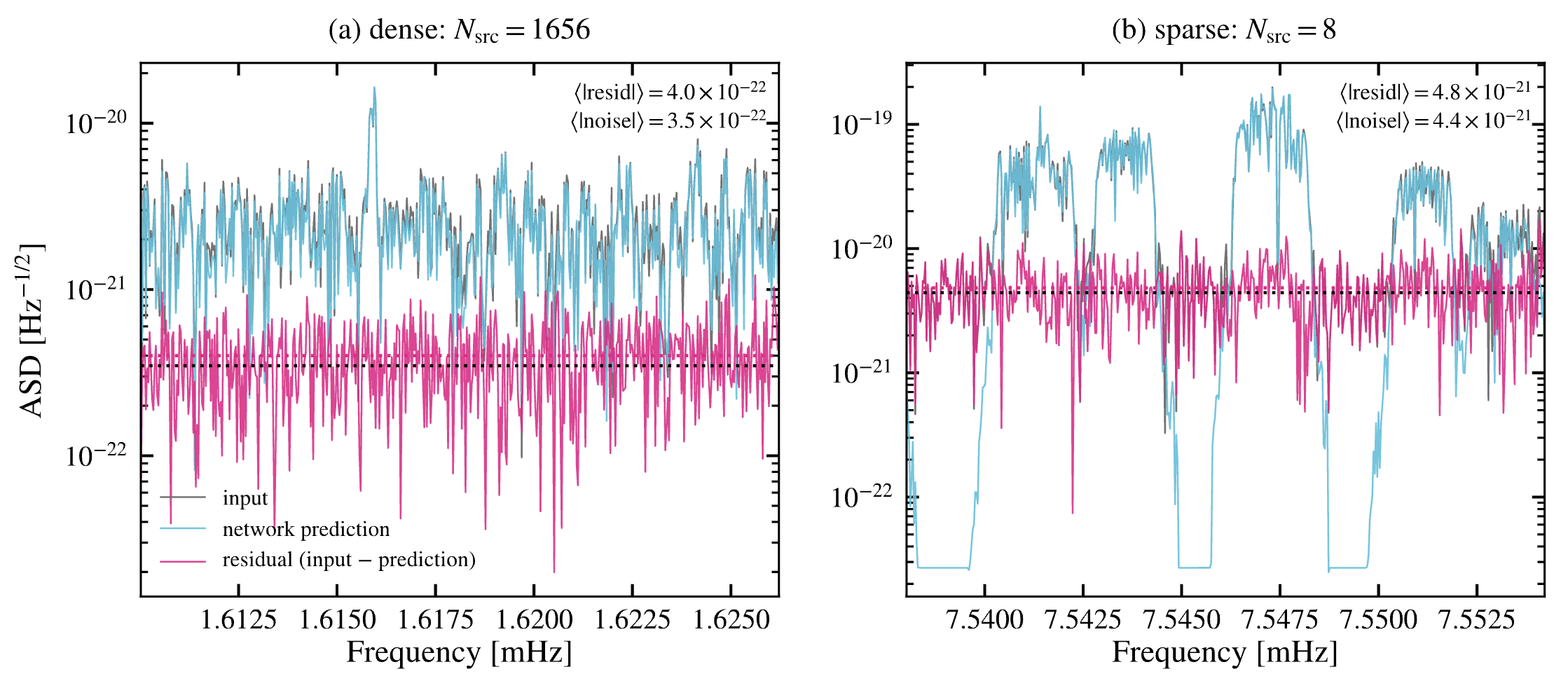
The goal is not to identify every binary, but to recover a noise-dominated residual.
Subtraction residual
Reconstructed GB foreground
Input GB foreground
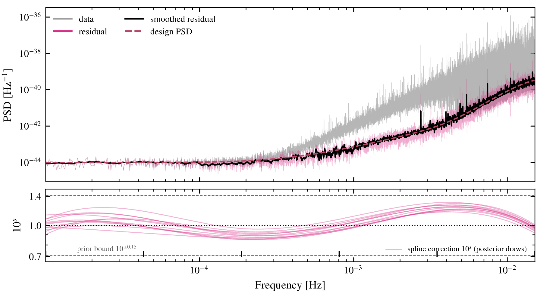
From 512-bin predictions to a continuous full-band residual
Sliding 512-bin windows are edge-cropped and stitched so that every frequency bin receives one reliable prediction.
Local predictions become one continuous residual across the full analysis band.
Full-band inference
- 512-bin sliding windows
- 10% edge crop: 51 bins per side
- stride: 410 bins
- reflection padding at the band boundaries
\(\hat g_c(f)=\operatorname{stitch}\left[M_{\rm GB}(d_c^{(w)})\right] \)
\(r_c(f)=d_c(f)-\hat g_c(f)\)
Instrumental PSD
Input GB foreground
Smoothed Residual
Only a small broadband mismatch remains.
One learned foreground model, three uses.
- Learn
population-conditioned training
\(\rightarrow\) frequency-bin–shared foreground network - Characterize
foreground-subtracted residual
\(\rightarrow\) unbiased \(A_{\rm acc}, A_{\rm oms}\) + bounded distortion - Deploy in-loop
cached subtraction inside MBHB MCMC
\(\rightarrow\) oracle-level posteriors
The learned foreground enters Bayesian inference
The same foreground model is reused for both noise characterization and source inference.
左侧图
四个块:
- GB catalog
- Instrument noise
- MBHB / EMRI / other targets
- Residual validation
箭头循环:
GB subtraction
$\rightarrow$ noise update
$\rightarrow$ target-source inference
$\rightarrow$ residual
$\rightarrow$ GB update
Katz, Karnesis, Korsakova, Gair, and Stergioulas (2025)
(adapted)
Learned
Foreground
Model
reused in
Pipeline overview
The learned foreground is reused—not retrained—inside downstream inference.
The learned foreground enters the likelihood
Every MCMC proposal is cleaned before evaluating the Whittle likelihood.
The sampler never fits the raw data — it fits the foreground-cleaned residual.
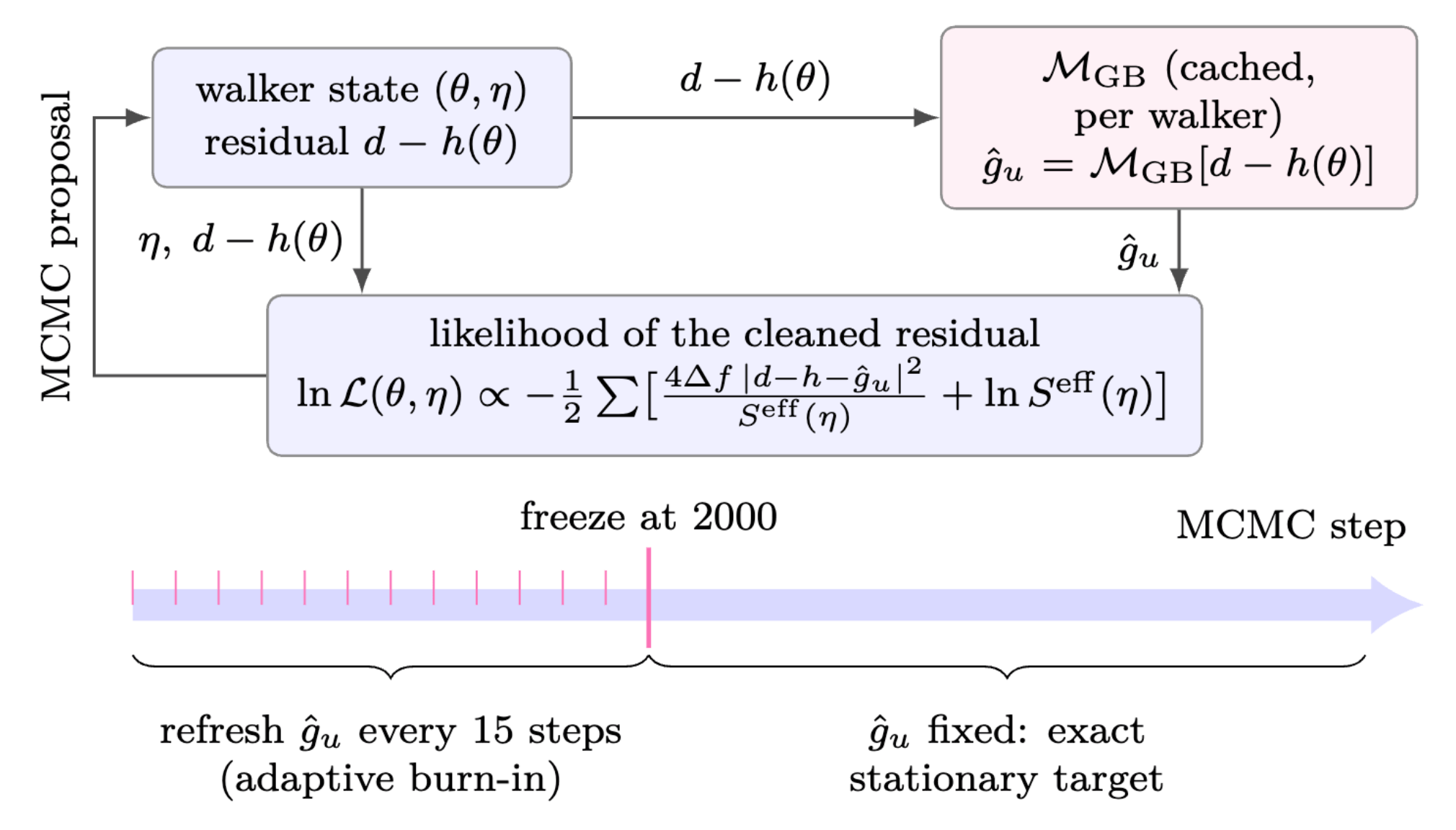
Model in the loop: The foreground prediction is refreshed every 15 iterations during burn-in and then frozen.
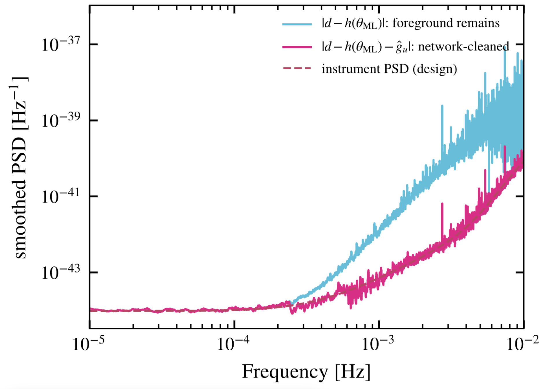
Every MCMC proposal is evaluated on the cleaned residual.
Foreground-cleaned residual
Turn the residual into a calibrated noise posterior.
From residual to noise posterior
The spline is the honesty knob: it absorbs residual subtraction bias.
\(\ln \mathcal{L} = -\frac{1}{2} \sum_f \left[ \ln S_{\rm eff}(f) + \frac{\widehat S_{\rm res}(f)}{S_{\rm eff}(f)} \right]\)
\(S_{\rm eff}(f) = S_A(f;A_{\rm acc},A_{\rm oms}) \,10^{s(\log_{10}f)}\)
Spline layer:
- 6 cubic knots
- hard bound: \(|y_m|\le0.15\)
- shrinkage + smoothness priors
- sampled jointly with noise amplitudes
We do not assume subtraction is perfect; we infer its smooth discrepancy.
Recovered noise amplitudes are consistent with injected design values.
Evidence II: unbiased noise parameters
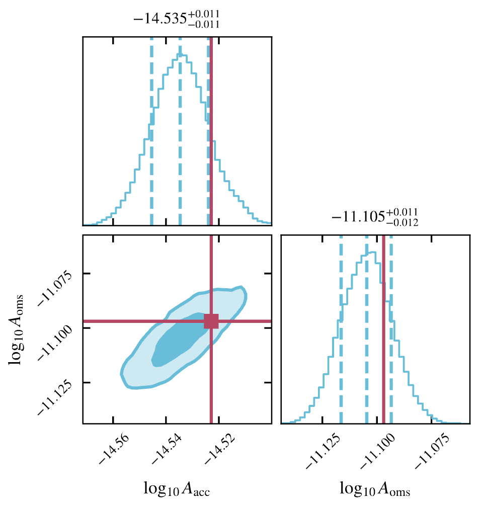
Foreground-subtracted residuals recover the injected Taiji noise amplitudes.
\(\log_{10}A_{\rm acc} = -14.535\pm0.011\)
\(\log_{10}A_{\rm oms} = -11.105\pm0.012\)
Injected:
\(\log_{10}(3\times10^{-15})=-14.523\)
\(\log_{10}(8\times10^{-12})=-11.097\)
Spline distortion:
bounded at roughly 15–30%
左:spectral residual + spline band;右:corner。标题下直接放结果数字。
The learned model’s systematic error is measured, not hidden.
Foreground-aware inference removes bias from both the noise and the source posterior
Correcting the foreground first restores both instrumental-noise calibration and MBHB parameter estimation.
??
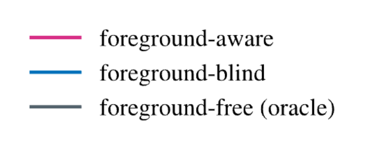
Noise characterization becomes unbiased
- recovered \(A_{\rm acc}\) and \(A_{\rm oms}\)
- posterior centered on the truth
- spline absorbs remaining smooth mismatch
- no systematic PSD inflation
MBHB posterior becomes unbiased
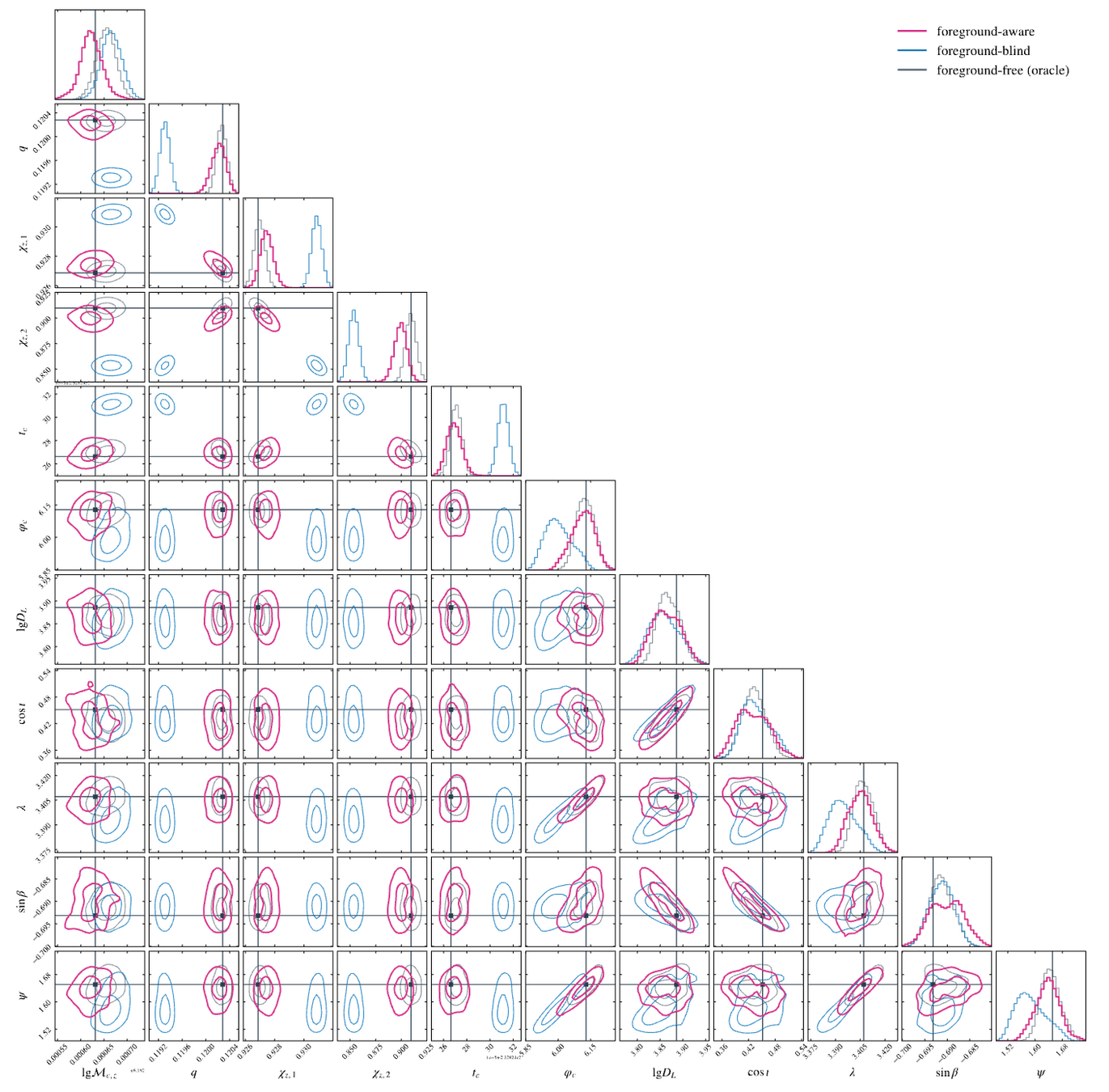
- intrinsic parameters: correct mode, slightly broader posterior
- extrinsic parameters: nearly oracle-equivalent
- residual foreground uncertainty is propagated, not hidden
Foreground-blind inference is confidently wrong.
Foreground-blind inference fails
Ignoring the foreground gives a confident but wrong posterior.
The likelihood assumes:
\(d = h_{\rm MBHB}(\theta) + n\)
but the data contain:
\(d = h_{\rm MBHB}(\theta) + g_{\rm GB} + n\)
Consequences:
- biased mass ratio
- biased spins
- shifted coalescence time
- biased sky/orientation angles
放 foreground-blind corner。只圈出最明显偏移参数,不要逐个讲全。
The problem is not larger uncertainty — it is many-\(\sigma\) bias.
Cached foreground subtraction inside MBHB MCMC
Model in the loop
Use the foreground model inside MCMC, but update it on a controlled schedule.
For each walker:
\(r^{(1)}(f|\theta)=d(f)-h(f|\theta)\)
\(\hat g_u(f)=M_{\rm GB}[d-h(\theta_u)]\)
\(r(f|\theta)=d(f)-h(f|\theta)-\hat g_u(f)\)
Schedule:
- refresh \(\hat g_u\) every 15 steps
- adaptive burn-in: first 2000 steps
- freeze \(\hat g_u\) for production: final 3000 steps
核心方法页。上方放 per-walker cache flow;中间放 refresh/freeze timeline;下方放 cleaned residual evidence 或小图。
Refresh for adaptation; freeze for a fixed stationary target.
Statistical role of the cached-update scheme
Why this is statistically honest
The adaptive part is burn-in; the production chain samples a fixed likelihood.
Caveats kept explicit:
- truth-local prior and initialization
- diagonal frequency covariance
- fixed even/odd walker identity
- foreground uncertainty not yet distributional
三列表格:phase / target / interpretation。右侧放 caveats 小框。
The network does not silently change the production target.
| Phase | Network cache | Interpretation |
|---|---|---|
| steps 0–2000 | refreshed every 15 steps | adaptive burn-in |
| steps 2000–5000 | fixed \(\hat g_u\) | exact stationary target |
| spline sampled jointly | absorbs smooth residual foreground | uncertainty propagation |
Foreground-aware inference restores oracle-level posteriors.
Evidence III: foreground-aware ≈ oracle
In-loop subtraction removes MBHB biases and recovers oracle-level posteriors.
Three analyses:
- Foreground-blind: no GB subtraction
- Foreground-aware: cached in-loop subtraction
- Foreground-free oracle: ideal GB removal
Main result:
many-\(\sigma\) biases disappear, foreground-aware posteriors overlap the oracle run.
全页放 three-run corner。颜色必须统一:blind 蓝、aware 品红、oracle 灰/黑。
The cost of not resolving \(4.5\times10^7\) sources is mainly a small posterior widening.
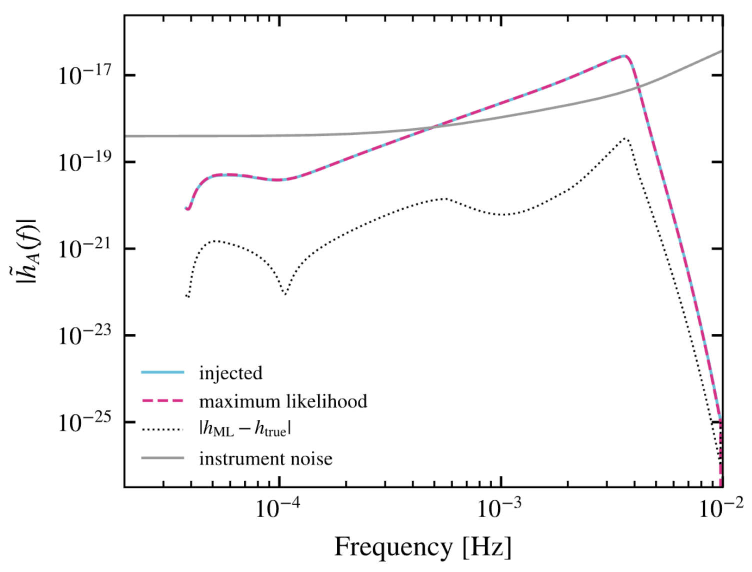
The maximum-likelihood waveform matches the injection.
Waveform-domain sanity check
The recovered parameters also reconstruct the waveform correctly.
\(|h_{\rm ML}-h_{\rm true}|\)
is
- below the signal
- below the instrument-noise level
- one to two orders of magnitude smaller across most of the band
放 injected vs ML waveform 图。右上角放结论短句。
The posterior recovery is not a parameter-space coincidence.
Calibrating learned systematic uncertainty
The learned foreground is not assumed perfect—its remaining error is explicitly calibrated and propagated into the posterior.
Existing uncertainty
- detector noise
- finite observation
- finite measurement precision
New uncertainty from learning
-
imperfect foreground prediction
-
residual foreground mismatch
↓
explicitly calibrated
Posterior interpretation
- bias largely removed
- remaining foreground uncertainty propagates into credible intervals
- intrinsic parameters become slightly broader
- no hidden over-confidence
Our goal is not to eliminate uncertainty, but to separate, calibrate, and propagate it honestly.
The maximum-likelihood waveform matches the injection.
The learned foreground closely reproduces the aggregate Galactic signal, while leaving only instrument-like residuals.
What did the model actually learn?
Where does the remaining uncertainty come from?
It learns a morphology-to-foreground operator rather than identifying individual binaries.
Global fit
- resolves bright sources
- outputs source catalog + posterior
- high computational cost
- scales with source number
Learned foreground operator
- maps data morphology to total foreground
- outputs \(\hat g(f)\) and residual
- one forward pass
- no individual source catalog
Center statement:
- Different question, complementary answer.
For noise characterization and target validation, the total foreground is often the object we need.
???
What “robust” means here — and what it does not yet mean
What “robust” means here
The model is robust to realization and density variation, but population mismatch remains open.
Robust by construction
- generative CNF resampling
- stochastic source counts
- dense-region focus sampling
- one network shared across the band
- Itakura–Saito residual calibration
- spline discrepancy layer
Open robustness axes
- different Galaxy populations
- gaps and glitches
- non-stationary instrument noise
- annual modulation and time dependence
- many-injection P–P validation
两列:Robust by construction / Not solved yet。
The spline is a first safety layer, not a substitute for population-level validation.
Dropping the learned operator into a global-fit workflow
Into a global-fit workflow
The learned model is best viewed as a fast block inside sequential/global-fit inference.
\(d \rightarrow M_{\rm GB} \rightarrow r \rightarrow (A_{\rm acc},A_{\rm oms},s) \rightarrow S_{\rm eff} \rightarrow \{\text{MBHB, bright GBs, EMRIs}\} \rightarrow d-h(\theta)\)
Roles:
- Initializer for classical GB blocks
- Surrogate for unresolved confusion during source sampling
- Validator for residuals after catalog subtraction
新绘闭环框图:data → foreground operator → residual → noise block → source blocks → subtraction → foreground operator。
Noise estimation, foreground subtraction, and source validation become coupled blocks of one sequential inference problem.
Toward weaker, longer-lived targets: the EMRI-like regime
Bonus: toward EMRI-like targets
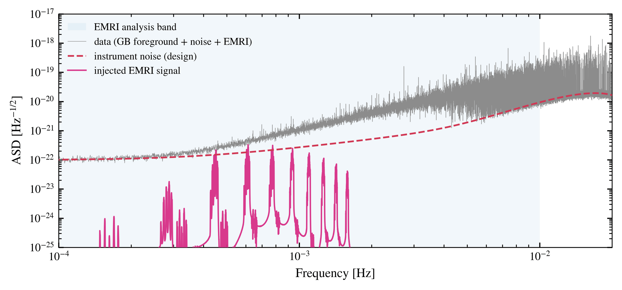
EMRIs are the natural next target because foreground bias accumulates over many cycles.
EMRI-like target
- months to years
- \(10^4\)–\(10^5\) cycles
- low instantaneous SNR
- foreground bias accumulates coherently
左右对比 MBHB vs EMRI-like。不要放复杂 EMRI 波形;用 conceptual timeline 更清楚。
MBHB is the first hard test; EMRI is the real stress test.
最好有EMRI的Result corner图
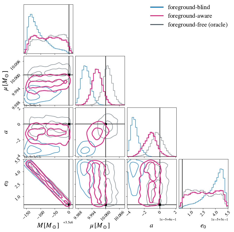
Needed extensions:
- distributional \(\hat g\)
- pseudo-marginal / variance-inflated likelihood
- time–frequency conditioning
- phase-coherent validation
Calibratable ML: a third way to put networks into inference
Calibratable machine learning
The key idea is not just using ML, but making ML error inferable.
End-to-end ML
network output \(\rightarrow\) detection / class / point estimate
Risk:
systematic error enters conclusions directly
ML-assisted sampler
Network \(\rightarrow\) proposal / surrogate / modified prior
Risk:
bias shapes exploration and is hard to audit
Calibratable ML
network output \(\rightarrow\) physical component of the data model
residual error \(\rightarrow\) explicit discrepancy model \(\rightarrow\) jointly inferred
Result:
measured
propagated
falsifiable
三栏对照表:end-to-end / ML-assisted sampling / calibratable ML。第三栏高亮。
A learned point estimate + an inferable discrepancy model.
Conclusions and outlook
Machine learning provides a practical and statistically honest bridge toward scalable LISA/Taiji global-fit inference.
✓ Learn the aggregate Galactic foreground, not individual binaries
✓ Recover unbiased instrumental-noise calibration
✓ Restore MBHB posterior consistency without source catalogs
Foreground estimation becomes an inference primitive.
Main contributions
AI learns NOT individual GB identities
↓
BUT a morphology → foreground map
↓
usable residuals for downstream inference
Different question, complementary answer.
What AI actually learned
Not every Galactic binary must be identified before precision inference becomes possible.
Conclusions and outlook
Machine learning provides a practical and statistically honest bridge toward scalable LISA/Taiji global-fit inference.
- The systematic error of the learned component becomes a target of Bayesian calibration.
Calibratable machine learning
- Gee-Moo for TDCII (with Jianan Zhang, ICTP-AP)
- MDP for global-fit (Frequentist vs Bayesian ...)
- ...
Ongoing work
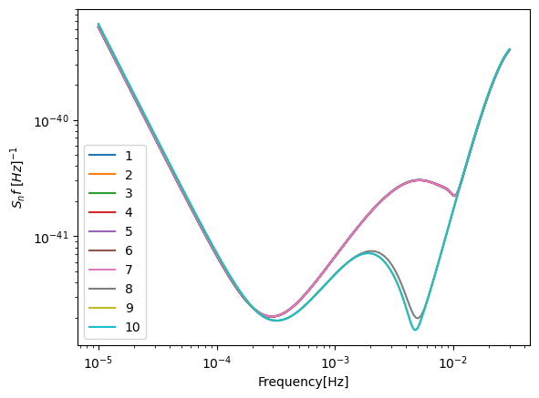
for _ in range(num_of_audiences):
    print('Thank you for your attention! 🙏')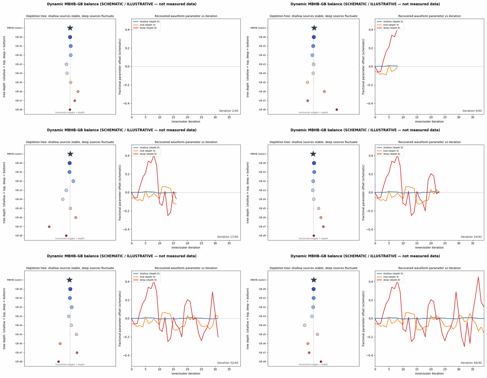
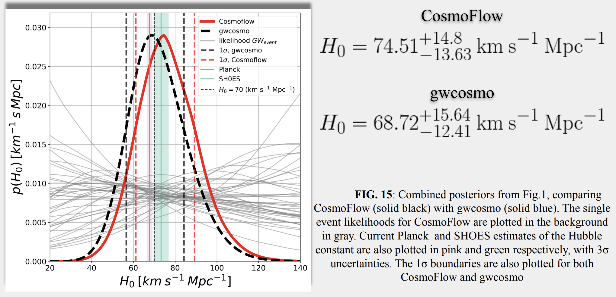
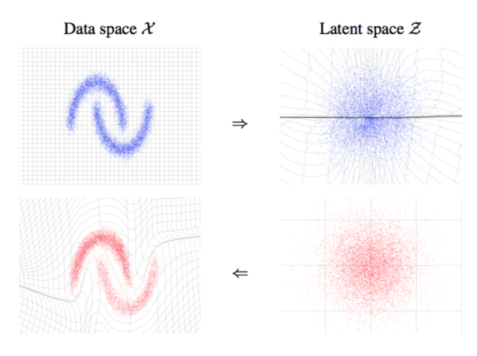
Stachurski+ (2024)
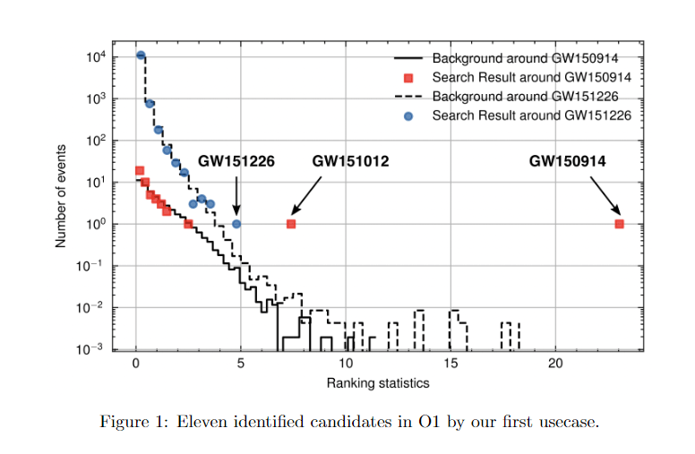
HW+ (2024)
Summary
End with three results and one conceptual takeaway.
- Foreground learning
One frequency-bin–shared network, trained on flow-generated foregrounds, subtracts \(10^7\)-source confusion to the noise floor. - Noise characterization
The residual recovers
\(\log_{10}A_{\rm acc}\) and \(\log_{10}A_{\rm oms}\)
with \(\pm0.011\) dex precision and bounded spline distortion. - Source inference
Cached in-loop subtraction removes many-\(\sigma\) MBHB biases and restores oracle-level posteriors.
三条 takeaway,每条配一个小缩略图:foreground subtraction / noise posterior / MBHB corner。底部 thank you。
The broader lesson:
learned operators can enter precision GW inference when their errors are calibrated, propagated, and falsifiable.