He Wang
hewang@ucas.ac.cn
International Centre for Theoretical Physics – Asia Pacific (ICTP-AP)
University of Chinese Academy of Sciences (UCAS)
25th Oct 2026 | ICFP 2026

Based on arXiv:2508.03661
Evo-MCTS: Gravitational-Wave Algorithm Search and Lessons for AI-Assisted Physics

hewang@ucas.ac.cn
AAD for GW detection Guided by LLM-informed Evo-MCTS
Our question
- Can we search for detection programs that experts can inspect and test?
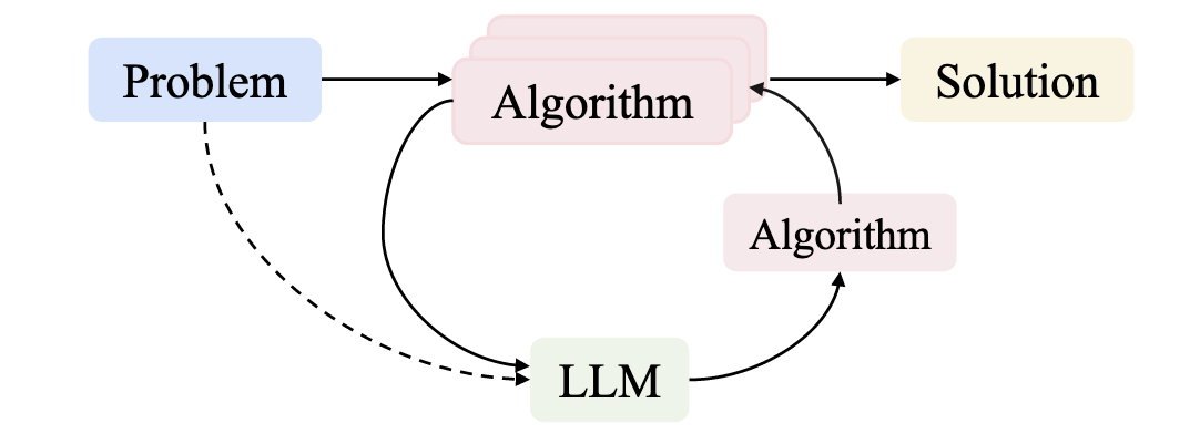
external_knowledge
(constraint)
Fitness
Challenges and Motivations
Matched filtering
- Sensitive to modeled signals, with computational costs that grow with template-bank coverage.
Neural networks
- Fast inference, with additional work needed to assess robustness and interpret learned decisions.
arXiv:2410.14716 [cs.LG]
Execute on benchmark data
LLM as designer
arXiv:2410.14716 [cs.LG]
import numpy as np
import scipy.signal as signal
def pipeline_v1(strain_h1: np.ndarray, strain_l1: np.ndarray, times: np.ndarray) -> tuple[np.ndarray, np.ndarray, np.ndarray]:
    def data_conditioning(strain_h1: np.ndarray, strain_l1: np.ndarray, times: np.ndarray) -> tuple[np.ndarray, np.ndarray, np.ndarray]:
        window_length = 4096
        dt = times[1] - times[0]
        fs = 1.0 / dt

        def whiten_strain(strain):
            strain_zeromean = strain - np.mean(strain)
            freqs, psd = signal.welch(strain_zeromean, fs=fs, nperseg=window_length,
                                       window='hann', noverlap=window_length//2)
            smoothed_psd = np.convolve(psd, np.ones(32) / 32, mode='same')
            smoothed_psd = np.maximum(smoothed_psd, np.finfo(float).tiny)
            white_fft = np.fft.rfft(strain_zeromean) / np.sqrt(np.interp(np.fft.rfftfreq(len(strain_zeromean), d=dt), freqs, smoothed_psd))
            return np.fft.irfft(white_fft)

        whitened_h1 = whiten_strain(strain_h1)
        whitened_l1 = whiten_strain(strain_l1)

        return whitened_h1, whitened_l1, times

    def compute_metric_series(h1_data: np.ndarray, l1_data: np.ndarray, time_series: np.ndarray) -> tuple[np.ndarray, np.ndarray]:
        fs = 1 / (time_series[1] - time_series[0])
        f_h1, t_h1, Sxx_h1 = signal.spectrogram(h1_data, fs=fs, nperseg=256, noverlap=128, mode='magnitude', detrend=False)
        f_l1, t_l1, Sxx_l1 = signal.spectrogram(l1_data, fs=fs, nperseg=256, noverlap=128, mode='magnitude', detrend=False)
        tf_metric = np.mean((Sxx_h1**2 + Sxx_l1**2) / 2, axis=0)
        gps_mid_time = time_series[0] + (time_series[-1] - time_series[0]) / 2
        metric_times = gps_mid_time + (t_h1 - t_h1[-1] / 2)

        return tf_metric, metric_times

    def calculate_statistics(tf_metric, t_h1):
        background_level = np.median(tf_metric)
        peaks, _ = signal.find_peaks(tf_metric, height=background_level * 1.0, distance=2, prominence=background_level * 0.3)
        peak_times = t_h1[peaks]
        peak_heights = tf_metric[peaks]
        peak_deltat = np.full(len(peak_times), 10.0)  # Fixed uncertainty value
        return peak_times, peak_heights, peak_deltat

    whitened_h1, whitened_l1, data_times = data_conditioning(strain_h1, strain_l1, times)
    tf_metric, metric_times = compute_metric_series(whitened_h1, whitened_l1, data_times)
    peak_times, peak_heights, peak_deltat = calculate_statistics(tf_metric, metric_times)

    return peak_times, peak_heights, peak_deltat
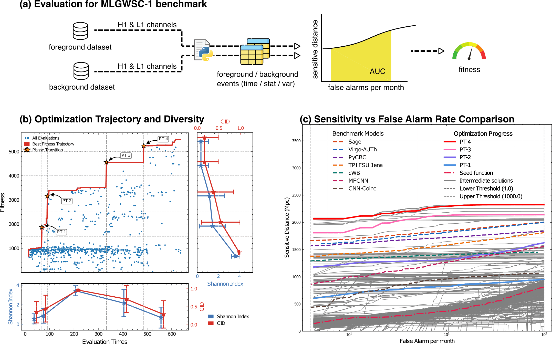
Optimization Target: Maximizing Area Under Curve (AUC) over the target false-alarm-rate range (e.g. 1–1000 false alarms/month), balancing detection sensitivity and false alarm rates across algorithm generations
The LLM does not predict answers — it reshapes how we search for algorithms.
Evo-MCTS searches over executable detection pipelines
HW & ZL, arXiv:2508.03661
external_knowledge
(constraint)

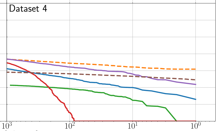



MLGWSC-1 benchmark
hewang@ucas.ac.cn
AAD for GW detection Guided by LLM-informed Evo-MCTS
LLM as designer
arXiv:2410.14716 [cs.LG]
The LLM does not predict answers — it reshapes how we search for algorithms.
Performance feedback guides the next code revision
HW & ZL, arXiv:2508.03661
external_knowledge
(constraint)
You are an expert in gravitational wave signal detection algorithms. Your task is to design heuristics that can effectively solve optimization problems.

{prompt_task}

I have analyzed two algorithms and provided a reflection on their differences.

[Worse code]
{worse_code}

[Better code]
{better_code}

[Reflection]
{reflection}

{external_knowledge}

Based on this reflection, please write an improved algorithm according to the reflection.
First, describe the design idea and main steps of your algorithm in one sentence. The description must be inside a brace outside the code implementation. Next, implement it in Python as a function named '{func_name}'.
This function should accept {input_count} input(s): {joined_inputs}. The function should return {output_count} output(s): {joined_outputs}.
{inout_inf} {other_inf}

Do not give additional explanations.
One Prompt Template for MLGWSC1 Algorithm Synthesis
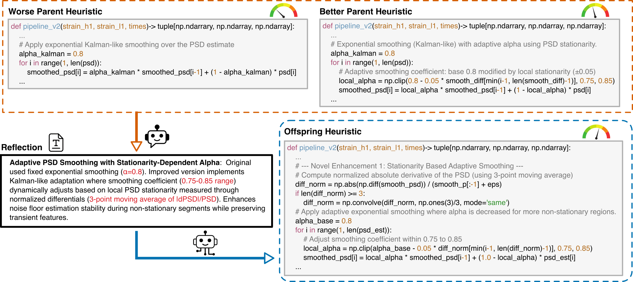
LLM-Driven Algorithmic Evolution Through Reflective Code Synthesis.
Algorithmic Synergy: MCTS, Evolution & LLM Agents
- Within each evolutionary iteration, MCTS decomposes complex signal detection problems into manageable decision sequences, enabling depth-wise and path-wise exploration of algorithmic possibilities.
- We propose four evolutionary operations for MCTS expansion: Parent Crossover (PC) combines information from nodes at the parent level, Sibling Crossover (SC) exchanges features between nodes sharing the same parent, Point Mutation (PM) introduces random perturbations to individual nodes, and Path-wise Crossover (PWC) synthesizes information along complete trajectories from root to leaf.
hewang@ucas.ac.cn
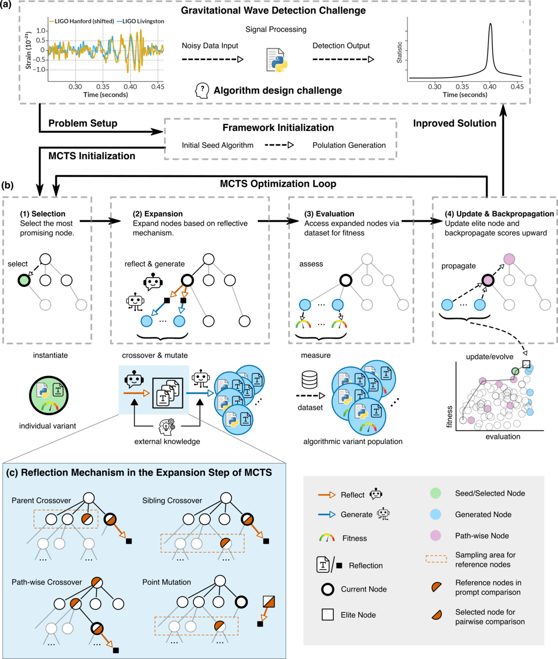
AAD for GW detection Guided by LLM-informed Evo-MCTS
Algorithmic Synergy: MCTS, Evolution & LLM Agents
hewang@ucas.ac.cn

- deepseek-R1 for reflection generation
- o3-mini-medium for code generation
- LLM-Driven Algorithmic Evolution Through Reflective Code Synthesis.
AAD for GW detection Guided by LLM-informed Evo-MCTS
MLGWSC1 Benchmark: Optimization Performance Results
hewang@ucas.ac.cn
HW & ZL, arXiv:2508.03661
AAD for GW detection Guided by LLM-informed Evo-MCTS
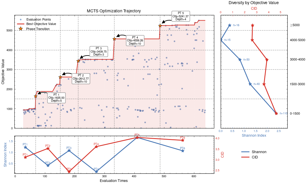
Automated exploration of algorithm parameter space
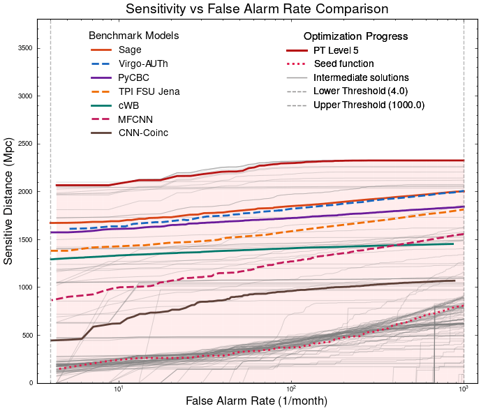
Benchmarking against state-of-the-art methods
MLGWSC1 Benchmark: Optimization Performance Results
hewang@ucas.ac.cn
HW & ZL, arXiv:2508.03661
AAD for GW detection Guided by LLM-informed Evo-MCTS
PyCBC (linear-core)
cWB (nonlinear-core)
Simple filters (non-linear)
CNN-like (highly non-linear)
Automated exploration of algorithm parameter space
Benchmarking against state-of-the-art methods
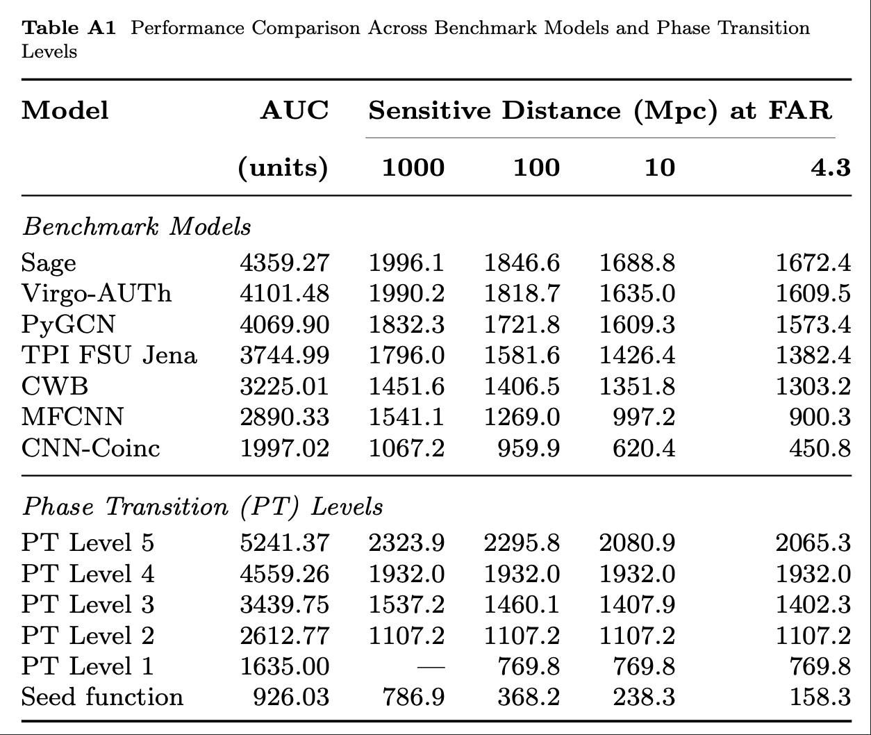
+20.2% benchmark AUC relative to Sage
~23% higher sensitive distance at FAR = 4.3/month
MLGWSC1 Benchmark: Optimization Performance Results
hewang@ucas.ac.cn
HW & ZL, arXiv:2508.03661
AAD for GW detection Guided by LLM-informed Evo-MCTS
PyCBC (linear-core)
cWB (nonlinear-core)
Simple filters (non-linear)
CNN-like (highly non-linear)
Automated exploration of algorithm parameter space
Benchmarking against state-of-the-art methods
20.2%
23.4%
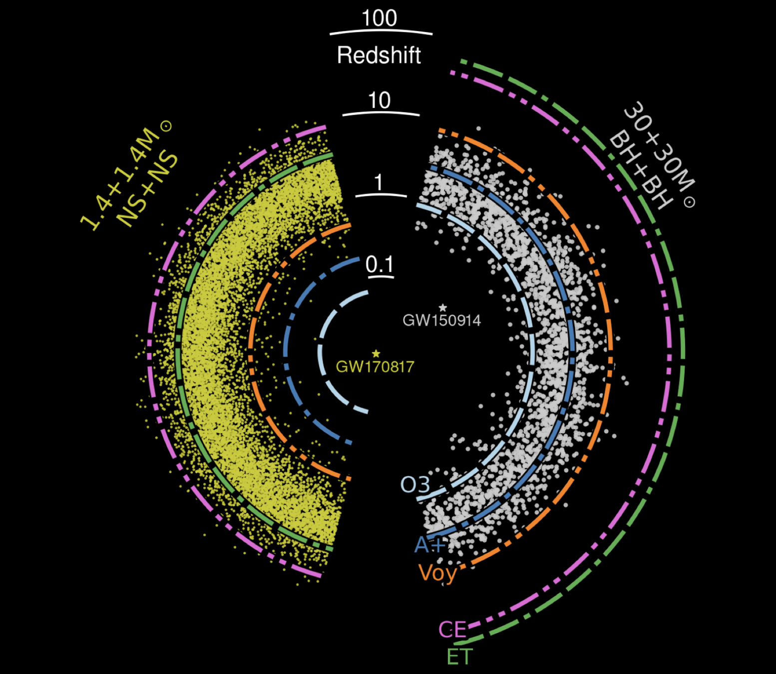
Understanding the search results
hewang@ucas.ac.cn
AAD for GW detection Guided by LLM-informed Evo-MCTS
Examining the generated programs and the evidence behind their performance
hewang@ucas.ac.cn
HW & ZL, arXiv:2508.03661
import numpy as np
import scipy.signal as signal
from scipy.signal.windows import tukey
from scipy.signal import savgol_filter

def pipeline_v2(strain_h1: np.ndarray, strain_l1: np.ndarray, times: np.ndarray) -> tuple[np.ndarray, np.ndarray, np.ndarray]:
    """
    The pipeline function processes gravitational wave data from the H1 and L1 detectors to identify potential gravitational wave signals.
    It takes strain_h1 and strain_l1 numpy arrays containing detector data, and times array with corresponding time points.
    The function returns a tuple of three numpy arrays: peak_times containing GPS times of identified events,
    peak_heights with significance values of each peak, and peak_deltat showing time window uncertainty for each peak.
    """
    eps = np.finfo(float).tiny
    dt = times[1] - times[0]
    fs = 1.0 / dt
    # Base spectrogram parameters
    base_nperseg = 256
    base_noverlap = base_nperseg // 2
    medfilt_kernel = 101       # odd kernel size for robust detrending
    uncertainty_window = 5     # half-window for local timing uncertainty

    # -------------------- Stage 1: Robust Baseline Detrending --------------------
    # Remove long-term trends using a median filter for each channel.
    detrended_h1 = strain_h1 - signal.medfilt(strain_h1, kernel_size=medfilt_kernel)
    detrended_l1 = strain_l1 - signal.medfilt(strain_l1, kernel_size=medfilt_kernel)

    # -------------------- Stage 2: Adaptive Whitening with Enhanced PSD Smoothing --------------------
    def adaptive_whitening(strain: np.ndarray) -> np.ndarray:
        # Center the signal.
        centered = strain - np.mean(strain)
        n_samples = len(centered)
        # Adaptive window length: between 5 and 30 seconds
        win_length_sec = np.clip(n_samples / fs / 20, 5, 30)
        nperseg_adapt = int(win_length_sec * fs)
        nperseg_adapt = max(10, min(nperseg_adapt, n_samples))

        # Create a Tukey window with 75% overlap.
        tukey_alpha = 0.25
        win = tukey(nperseg_adapt, alpha=tukey_alpha)
        noverlap_adapt = int(nperseg_adapt * 0.75)
        if noverlap_adapt >= nperseg_adapt:
            noverlap_adapt = nperseg_adapt - 1

        # Estimate the power spectral density (PSD) using Welch's method.
        freqs, psd = signal.welch(centered, fs=fs, nperseg=nperseg_adapt,
                                  noverlap=noverlap_adapt, window=win, detrend='constant')
        psd = np.maximum(psd, eps)

        # Compute relative differences for PSD stationarity measure.
        diff_arr = np.abs(np.diff(psd)) / (psd[:-1] + eps)
        # Smooth the derivative with a moving average.
        if len(diff_arr) >= 3:
            smooth_diff = np.convolve(diff_arr, np.ones(3)/3, mode='same')
        else:
            smooth_diff = diff_arr

        # Exponential smoothing (Kalman-like) with adaptive alpha using PSD stationarity.
        smoothed_psd = np.copy(psd)
        for i in range(1, len(psd)):
            # Adaptive smoothing coefficient: base 0.8 modified by local stationarity (±0.05)
            local_alpha = np.clip(0.8 - 0.05 * smooth_diff[min(i-1, len(smooth_diff)-1)], 0.75, 0.85)
            smoothed_psd[i] = local_alpha * smoothed_psd[i-1] + (1 - local_alpha) * psd[i]

        # Compute Tikhonov regularization gain based on deviation from median PSD.
        noise_baseline = np.median(smoothed_psd)
        raw_gain = (smoothed_psd / (noise_baseline + eps)) - 1.0

        # Compute a causal-like gradient using the Savitzky-Golay filter.
        win_len = 11 if len(smoothed_psd) >= 11 else ((len(smoothed_psd)//2)*2+1)
        polyorder = 2 if win_len > 2 else 1
        delta_freq = np.mean(np.diff(freqs))
        grad_psd = savgol_filter(smoothed_psd, win_len, polyorder, deriv=1, delta=delta_freq, mode='interp')

        # Nonlinear scaling via sigmoid to enhance gradient differences.
        sigmoid = lambda x: 1.0 / (1.0 + np.exp(-x))
        scaling_factor = 1.0 + 2.0 * sigmoid(np.abs(grad_psd) / (np.median(smoothed_psd) + eps))

        # Compute adaptive gain factors with nonlinear scaling.
        gain = 1.0 - np.exp(-0.5 * scaling_factor * raw_gain)
        gain = np.clip(gain, -8.0, 8.0)

        # FFT-based whitening: interpolate gain and PSD onto FFT frequency bins.
        signal_fft = np.fft.rfft(centered)
        freq_bins = np.fft.rfftfreq(n_samples, d=dt)
        interp_gain = np.interp(freq_bins, freqs, gain, left=gain[0], right=gain[-1])
        interp_psd = np.interp(freq_bins, freqs, smoothed_psd, left=smoothed_psd[0], right=smoothed_psd[-1])
        denom = np.sqrt(interp_psd) * (np.abs(interp_gain) + eps)
        denom = np.maximum(denom, eps)
        white_fft = signal_fft / denom
        whitened = np.fft.irfft(white_fft, n=n_samples)
        return whitened

    # Whiten H1 and L1 channels using the adapted method.
    white_h1 = adaptive_whitening(detrended_h1)
    white_l1 = adaptive_whitening(detrended_l1)

    # -------------------- Stage 3: Coherent Time-Frequency Metric with Frequency-Conditioned Regularization --------------------
    def compute_coherent_metric(w1: np.ndarray, w2: np.ndarray) -> tuple[np.ndarray, np.ndarray]:
        # Compute complex spectrograms preserving phase information.
        f1, t_spec, Sxx1 = signal.spectrogram(w1, fs=fs, nperseg=base_nperseg,
                                              noverlap=base_noverlap, mode='complex', detrend=False)
        f2, t_spec2, Sxx2 = signal.spectrogram(w2, fs=fs, nperseg=base_nperseg,
                                               noverlap=base_noverlap, mode='complex', detrend=False)
        # Ensure common time axis length.
        common_len = min(len(t_spec), len(t_spec2))
        t_spec = t_spec[:common_len]
        Sxx1 = Sxx1[:, :common_len]
        Sxx2 = Sxx2[:, :common_len]

        # Compute phase differences and coherence between detectors.
        phase_diff = np.angle(Sxx1) - np.angle(Sxx2)
        phase_coherence = np.abs(np.cos(phase_diff))

        # Estimate median PSD per frequency bin from the spectrograms.
        psd1 = np.median(np.abs(Sxx1)**2, axis=1)
        psd2 = np.median(np.abs(Sxx2)**2, axis=1)

        # Frequency-conditioned regularization gain (reflection-guided).
        lambda_f = 0.5 * ((np.median(psd1) / (psd1 + eps)) + (np.median(psd2) / (psd2 + eps)))
        lambda_f = np.clip(lambda_f, 1e-4, 1e-2)
        # Regularization denominator integrating detector PSDs and lambda.
        reg_denom = (psd1[:, None] + psd2[:, None] + lambda_f[:, None] + eps)

        # Weighted phase coherence that balances phase alignment with noise levels.
        weighted_comp = phase_coherence / reg_denom

        # Compute axial (frequency) second derivatives as curvature estimates.
        d2_coh = np.gradient(np.gradient(phase_coherence, axis=0), axis=0)
        avg_curvature = np.mean(np.abs(d2_coh), axis=0)

        # Nonlinear activation boost using tanh for regions of high curvature.
        nonlinear_boost = np.tanh(5 * avg_curvature)
        linear_boost = 1.0 + 0.1 * avg_curvature

        # Cross-detector synergy: weight derived from global median consistency.
        novel_weight = np.mean((np.median(psd1) + np.median(psd2)) / (psd1[:, None] + psd2[:, None] + eps), axis=0)

        # Integrated time-frequency metric combining all enhancements.
        tf_metric = np.sum(weighted_comp * linear_boost * (1.0 + nonlinear_boost), axis=0) * novel_weight

        # Adjust the spectrogram time axis to account for window delay.
        metric_times = t_spec + times[0] + (base_nperseg / 2) / fs
        return tf_metric, metric_times

    tf_metric, metric_times = compute_coherent_metric(white_h1, white_l1)

    # -------------------- Stage 4: Multi-Resolution Thresholding with Octave-Spaced Dyadic Wavelet Validation --------------------
    def multi_resolution_thresholding(metric: np.ndarray, times_arr: np.ndarray) -> tuple[np.ndarray, np.ndarray, np.ndarray]:
        # Robust background estimation with median and MAD.
        bg_level = np.median(metric)
        mad_val = np.median(np.abs(metric - bg_level))
        robust_std = 1.4826 * mad_val
        threshold = bg_level + 1.5 * robust_std

        # Identify candidate peaks using prominence and minimum distance criteria.
        peaks, _ = signal.find_peaks(metric, height=threshold, distance=2, prominence=0.8 * robust_std)
        if peaks.size == 0:
            return np.array([]), np.array([]), np.array([])

        # Local uncertainty estimation using a Gaussian-weighted convolution.
        win_range = np.arange(-uncertainty_window, uncertainty_window + 1)
        sigma = uncertainty_window / 2.5
        gauss_kernel = np.exp(-0.5 * (win_range / sigma) ** 2)
        gauss_kernel /= np.sum(gauss_kernel)
        weighted_mean = np.convolve(metric, gauss_kernel, mode='same')
        weighted_sq = np.convolve(metric ** 2, gauss_kernel, mode='same')
        variances = np.maximum(weighted_sq - weighted_mean ** 2, 0.0)
        uncertainties = np.sqrt(variances)
        uncertainties = np.maximum(uncertainties, 0.01)

        valid_times = []
        valid_heights = []
        valid_uncerts = []
        n_metric = len(metric)

        # Compute a simple second derivative for local curvature checking.
        if n_metric > 2:
            second_deriv = np.diff(metric, n=2)
            second_deriv = np.pad(second_deriv, (1, 1), mode='edge')
        else:
            second_deriv = np.zeros_like(metric)

        # Use octave-spaced scales (dyadic wavelet validation) to validate peak significance.
        widths = np.arange(1, 9)  # approximate scales 1 to 8
        for peak in peaks:
            # Skip peaks lacking sufficient negative curvature.
            if second_deriv[peak] > -0.1 * robust_std:
                continue
            local_start = max(0, peak - uncertainty_window)
            local_end = min(n_metric, peak + uncertainty_window + 1)
            local_segment = metric[local_start:local_end]
            if len(local_segment) < 3:
                continue
            try:
                cwt_coeff = signal.cwt(local_segment, signal.ricker, widths)
            except Exception:
                continue
            max_coeff = np.max(np.abs(cwt_coeff))
            # Threshold for validating the candidate using local MAD.
            cwt_thresh = mad_val * np.sqrt(2 * np.log(len(local_segment) + eps))
            if max_coeff >= cwt_thresh:
                valid_times.append(times_arr[peak])
                valid_heights.append(metric[peak])
                valid_uncerts.append(uncertainties[peak])

        if len(valid_times) == 0:
            return np.array([]), np.array([]), np.array([])
        return np.array(valid_times), np.array(valid_heights), np.array(valid_uncerts)

    peak_times, peak_heights, peak_deltat = multi_resolution_thresholding(tf_metric, metric_times)
    return peak_times, peak_heights, peak_deltat
Example candidate program
LLM-Guided Search in Program Space
HW & ZL, arXiv:2508.03661
AAD for GW detection Guided by LLM-informed Evo-MCTS
Intelligent guidance does not eliminate trial-and-error search.
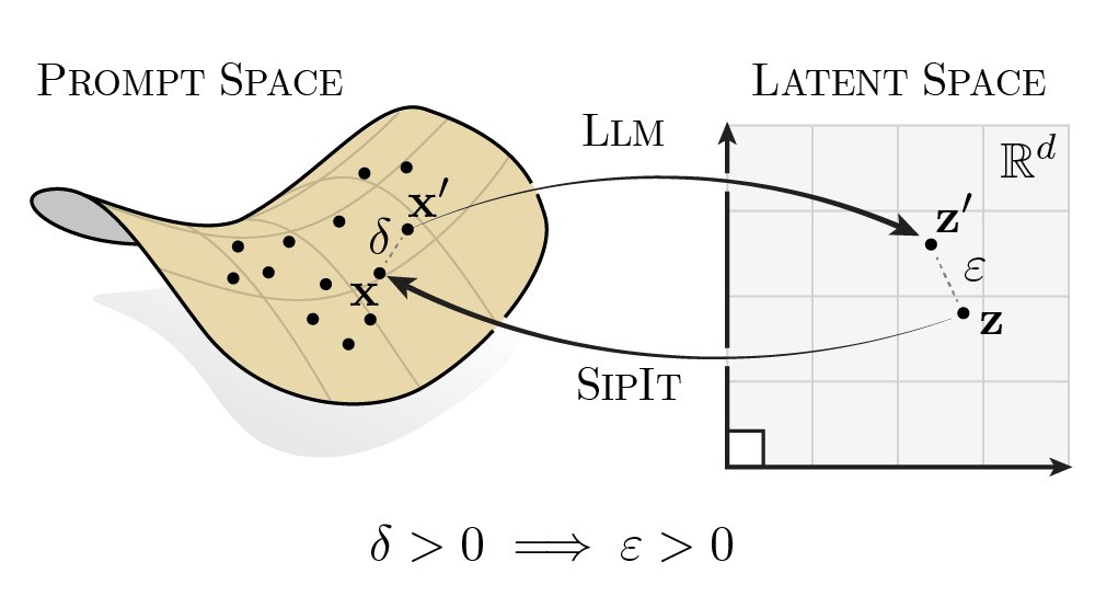
Algorithmic Space
Prompt/Knowledge Space
NLP
execute + evaluate
solution
Lesson 1: Guided brute-force search in program space
- LLMs propose programs rather than directly solving the scientific problem.
- Evolutionary strategies and MCTS guide the search through executable candidates.
- Much of this process can be viewed as recombination and “interpolation” of existing knowledge.
YouTube (Source)
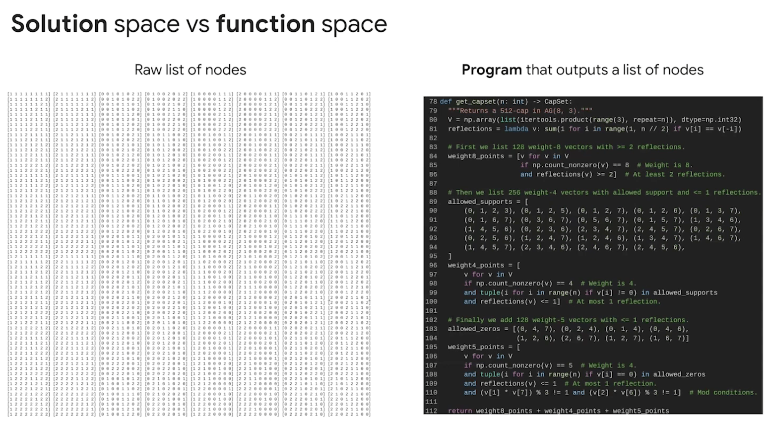
From Solutions to Programs: FunSearch
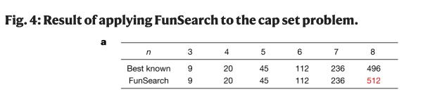

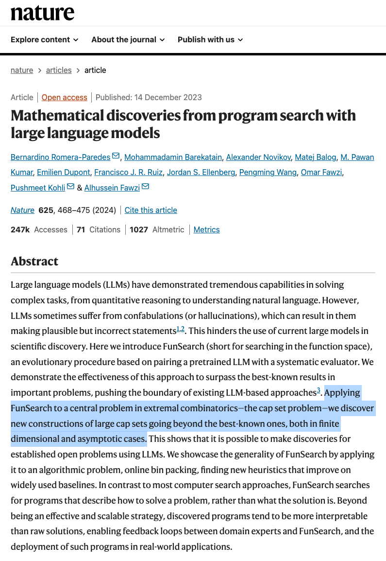
LLM guided search in program space
Interpretability Analysis
Out-of-distribution (OOD) detection
- Generalization capability and robustness of the optimized algorithms
hewang@ucas.ac.cn
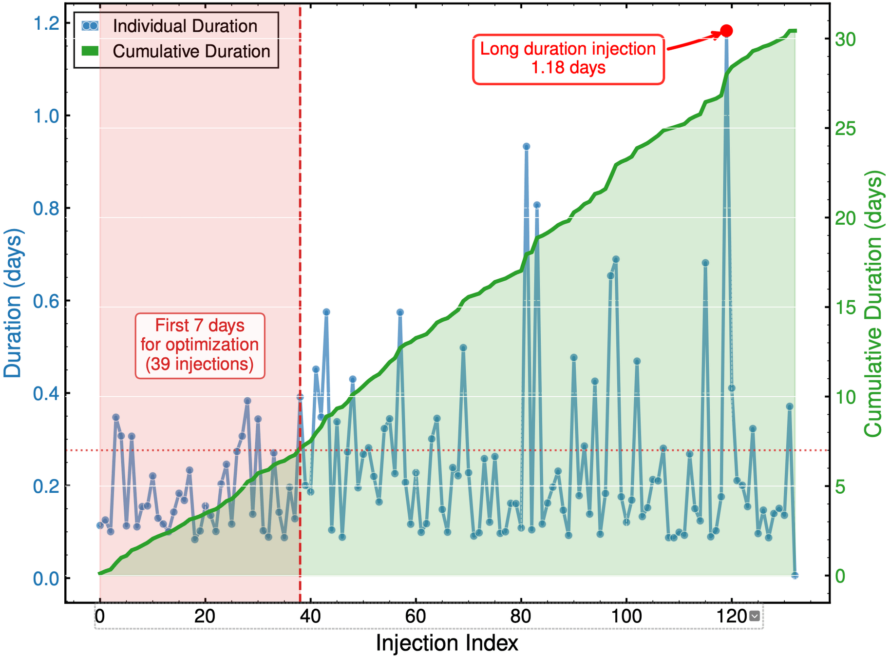
HW & ZL, arXiv:2508.03661
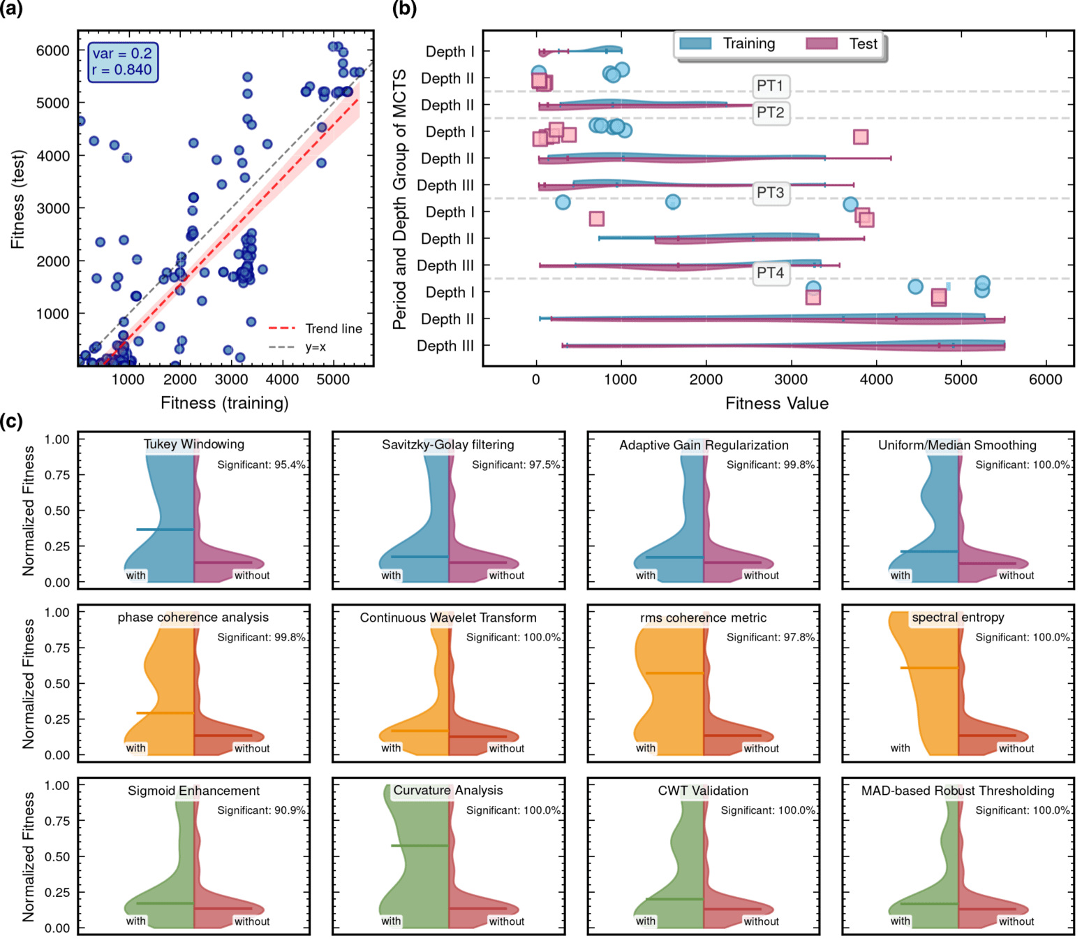
MCTS Depth-Stratified Performance Analysis.
- Analyzed the relationship between MCTS tree depth and algorithm fitness across different optimization phases. The 10-layer MCTS structure was stratified into three depth groups: Depth I (depths 1-4), Depth II (depths 5-7), and Depth III (depths 8-10), representing shallow, intermediate, and deep exploration levels, respectively.
Algorithmic Component Impact Analysis.
- A comprehensive technique impact analysis using controlled comparative methodology
AAD for GW detection Guided by LLM-informed Evo-MCTS
hewang@ucas.ac.cn
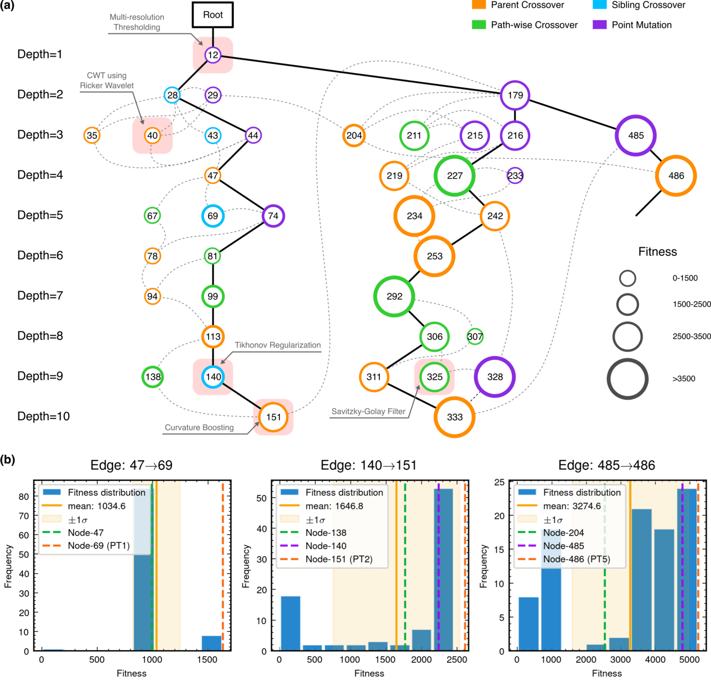
Evolutionary search guided by MCTS
- Each node represents an executable candidate program.
- Colors indicate different evolutionary operations.
- Node size reflects benchmark fitness.
-
The search history reveals how algorithms evolve through successive revisions.
AAD for GW detection Guided by LLM-informed Evo-MCTS
HW & ZL, arXiv:2508.03661
Tracing the Evolution of a Detection Program
HW & ZL, arXiv:2508.03661
The search history reveals how algorithms evolve through successive revisions.
hewang@ucas.ac.cn
Developed in 2024, Evo-MCTS combined evolutionary algorithms, Monte Carlo Tree Search, and LLM-driven code generation.
Lesson 2: In retrospect, it already embodied the core architecture of today’s AI research agents.
AI Agent = LLMs + Harness
Harness = Search + Execution + Evaluation + Feedback
Toward self-improving research agents: Can the search process itself become an optimization target?
AAD for GW detection Guided by LLM-informed Evo-MCTS
HW & ZL, arXiv:2508.03661
Evo-MCTS: An Early Form of AI Research Agent
HW & ZL, arXiv:2508.03661
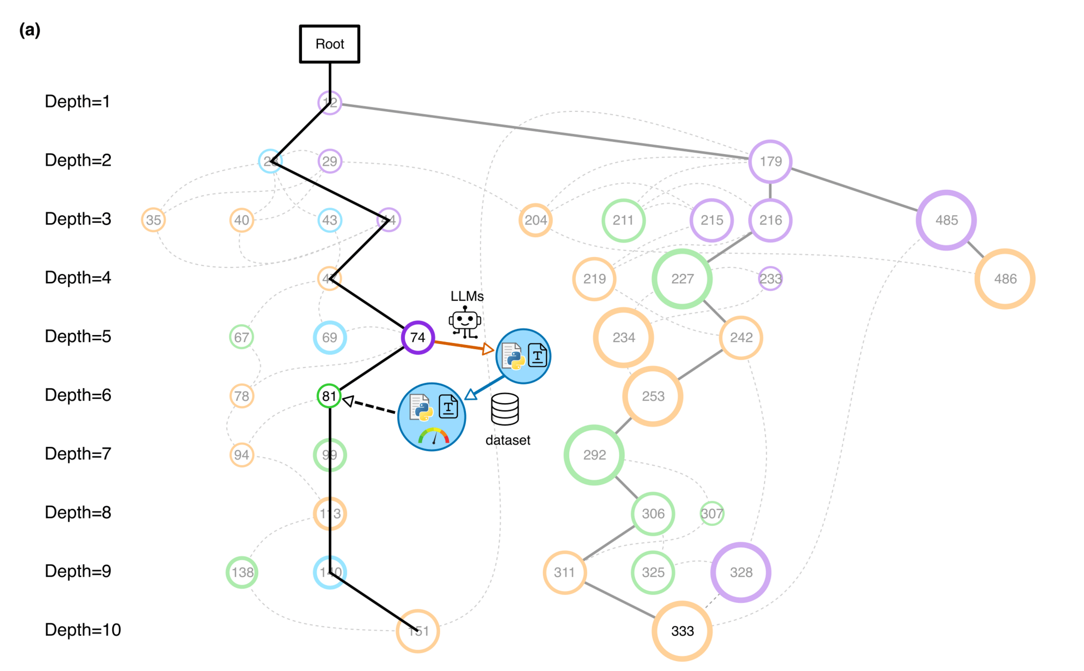
Interpretability Analysis
hewang@ucas.ac.cn
HW & ZL, arXiv:2508.03661
MCTS Algorithmic Evolution Pathway
- Complete MCTS tree structure showing all nodes associated with the optimal algorithm.
AAD for GW detection Guided by LLM-informed Evo-MCTS
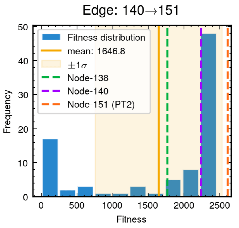
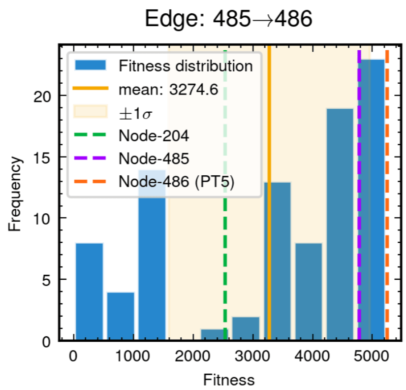
Edge robustness analysis for three critical evolutionary transitions.
- Confirming the consistent discovery
Interpretability Analysis
hewang@ucas.ac.cn
HW & ZL, arXiv:2508.03661
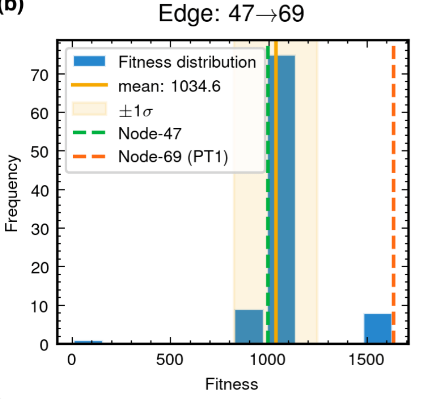
Edge robustness analysis for three critical evolutionary transitions.
- The distributions demonstrate the stochastic nature of LLM-driven code generation while confirming the consistent discovery of high-performance algorithmic variants.
AAD for GW detection Guided by LLM-informed Evo-MCTS
hewang@ucas.ac.cn
HW & ZL, arXiv:2508.03661
From Predictive Models to Algorithm Discovery
HW & ZL, arXiv:2508.03661
AAD for GW detection Guided by LLM-informed Evo-MCTS
Lesson 3: AI can optimize not only model parameters, but also the structure of scientific algorithms.
Program-Based AI Approach
The best of both worlds
Input
Physics-Informed
Algorithm
(High interpretability)
Output
Example: Evo-MCTS,
AlphaEvolve
AI Model
Physics
Knowledge
Black-Box AI Approach
Input
AI Model
(Low interpretability)
Output
Examples: CNN, AlphaFold
Data/
Experience
🎯 OUR WORK
|
Optimize model parameters |
Optimize program structure and parameters |
|
Produce a trained model |
Produce executable analysis code |
|
Examine model behavior |
Inspect code and test individual components |
Learning a predictor
Searching for a program
Explicit programs enable inspection, modification, and targeted validation.
Scientific discovery involves many processes that can be formulated as search and optimization problems.
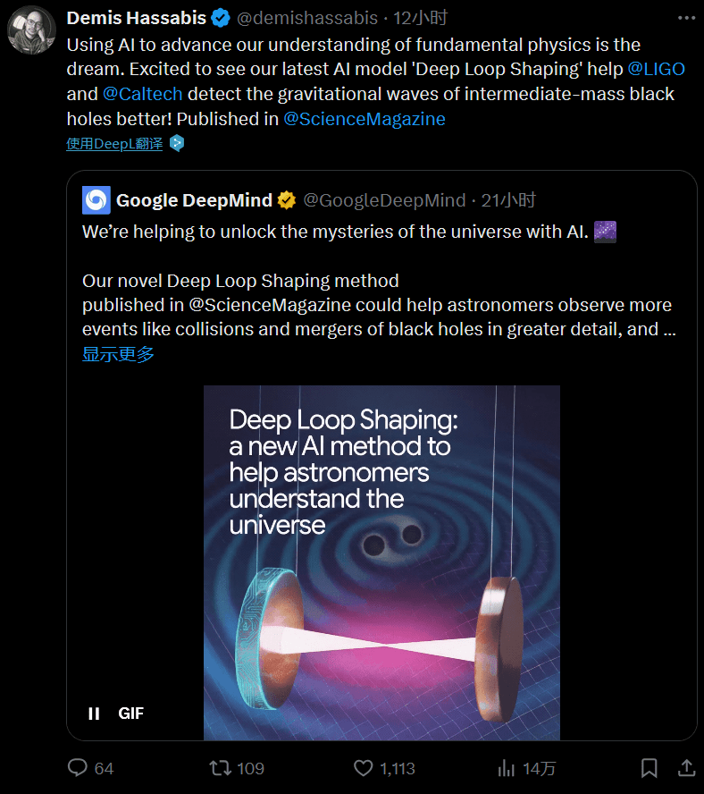
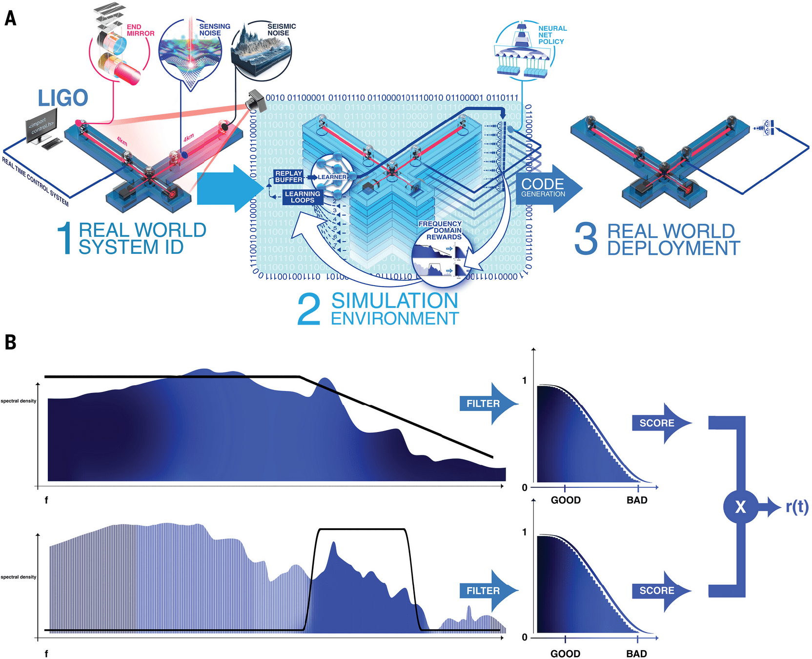
Scientific discovery itself may still offer vast, largely unexplored opportunities for optimization.
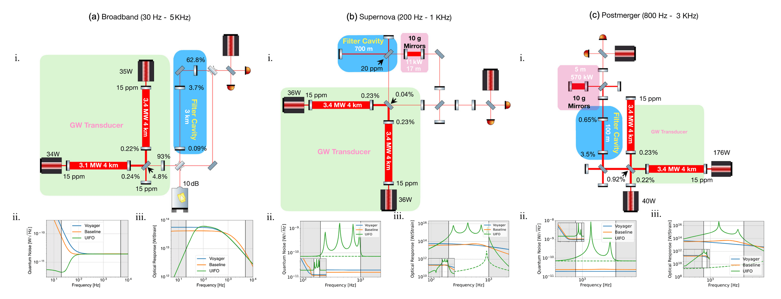
Krenn, Drori & Adhikari, Phys. Rev. X 15, 021012 (2025).
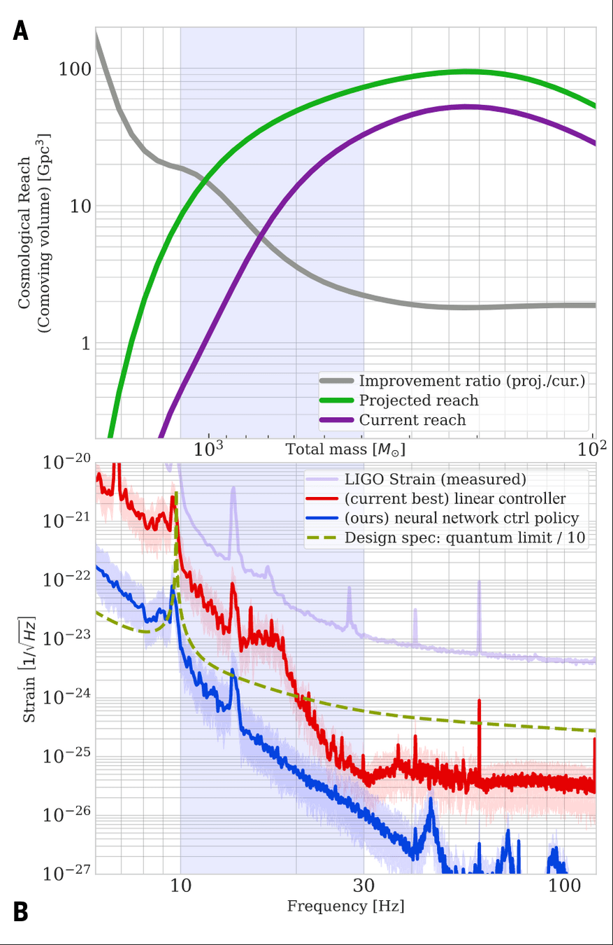
Buchli et al., Science 389, 1012–1015 (2025).
Searching for Scientific Discoveries
- Case 1 — AI-driven experiment design
- Experiment design as optimization
- The search object is no longer a parameter vector — it can be the experiment itself.
- Case 2 — Deep Loop Shaping for LIGO
- simulation-trained controller → real LIGO deployment
- The discovered object is a control policy, not a prediction.
hewang@ucas.ac.cn
Takeaways: From Algorithm Search to AI-Assisted Science
Takeaways
-
Guided Search, Not Magic
LLM-driven discovery remains largely a guided search over programs, building on existing knowledge.
-
From Evo-MCTS to Research Agents
Evolutionary search, MCTS, LLMs, and evaluation harnesses already form the basis of an autonomous research loop.
-
Beyond Algorithm Discovery
Scientific research may contain far more optimizable structures and processes than we currently exploit.
AAD for GW detection Guided by LLM-informed Evo-MCTS
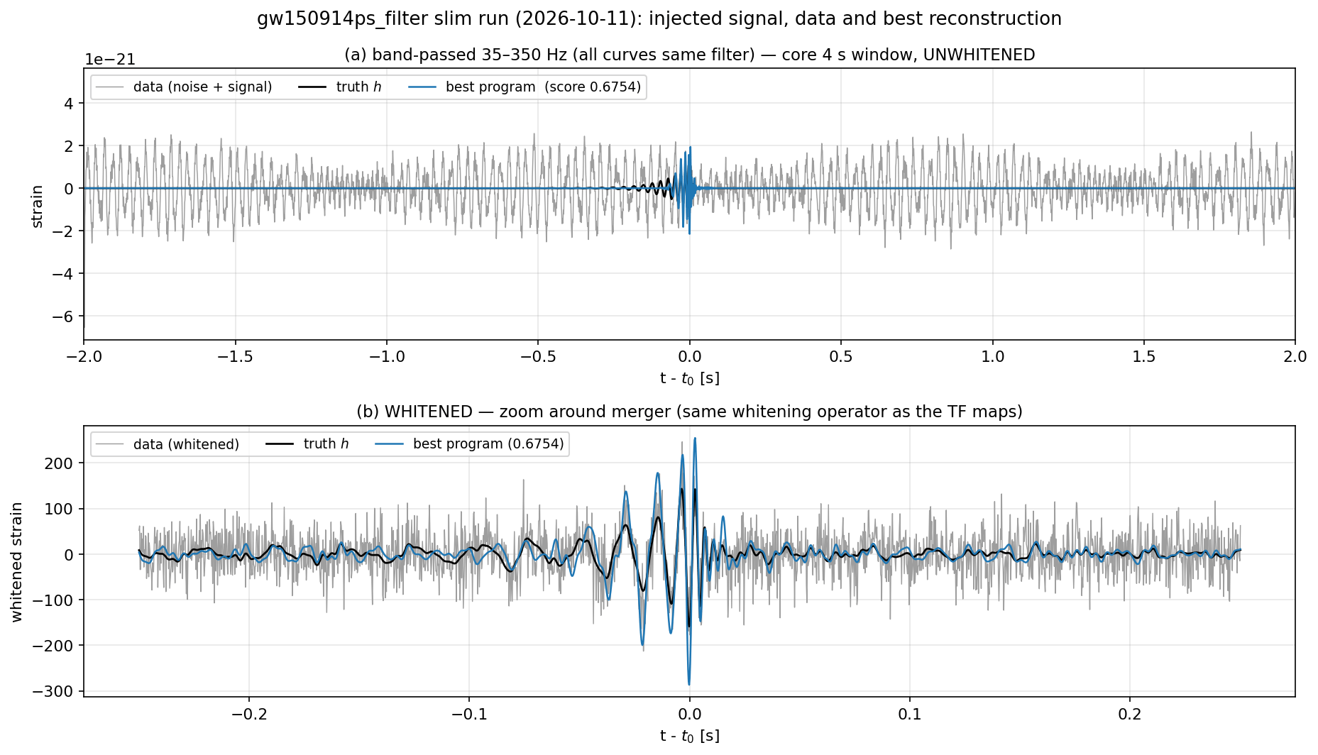
Current Research
Formal Verification in Theoretical Physics
Lean 4 formalization of black-hole solutions and perturbation identities.
Automated Gravitational-Wave Algorithm Discovery
Searching for improved event-specific denoising and signal-processing strategies.
Our aim is to connect automated search with independently checkable scientific claims.
Completed: Lean verification of matrix integrating-factor identities and local equivalence for Kerr–Newman perturbation systems. Ref: Hintz (2026)


PRELIMINARY
PRELIMINARY
AAD for GW detection Guided by LLM-informed Evo-MCTS
Takeaways: From Algorithm Search to AI-Assisted Science
Takeaways
-
Guided Search, Not Magic
LLM-driven discovery remains largely a guided search over programs, building on existing knowledge.
-
From Evo-MCTS to Research Agents
Evolutionary search, MCTS, LLMs, and evaluation harnesses already form the basis of an autonomous research loop.
-
Beyond Algorithm Discovery
Scientific research may contain far more optimizable structures and processes than we currently exploit.
Current Research
Formal Verification in Theoretical Physics
Lean 4 formalization of black-hole solutions and perturbation identities.
Automated Gravitational-Wave Algorithm Discovery
Searching for improved event-specific denoising and signal-processing strategies.
Our aim is to connect automated search with independently checkable scientific claims.
Completed: Lean verification of matrix integrating-factor identities and local equivalence for Kerr–Newman perturbation systems. Ref: Hintz (2026)
PRELIMINARY
hewang@ucas.ac.cn

for _ in range(num_of_audiences):
    print('Thank you for your attention! 🙏')