Research on Intelligent Noise Reduction and Parameter Estimation in Gravitational Wave Detection
王赫 (He Wang)
合作导师:何吉波 教授


Postdoctoral Defense
Email: hewang@ucas.ac.cn
June 18, 2024 (Location: Beijing, China)
Ground-based GW search and denoising, along with parameter estimation in space-based GW project.
主要是你要考虑吴老师他们的背景,然后简明扼要,突出亮点。讲的时间不要超过30分钟,能20+讲完更好。感觉吴老师抽出一个小时都比较困难……
- 地面引力波探测
- background
- detection & denoising (WaveFormer)
- 空间引力波探测
- background
- nflow + tingo 工作
- global-fit review
- on-going work for global-fit
- 总结
- AI+earth-based (提及最前沿进展和自己的位置+2年接触的工作+数据平台)
- AI+space-based (提及最前沿进展和国内的位置+2年接触的工作,还有太极天琴的位置,训练营培训+正在的学生课题,科创计划,数据开源平台)
- non-GW
- NeuTra-lizing Bad Geometry in Hamiltonian Monte Carlo Using Neural Transport (1903.03704 )
- Accelerated Bayesian inference using deep learning (https://doi.org/10.1093/mnras/staa1469)
- Nested Sampling Methods (2101.09675)
- pocoMC: A Python package for accelerated Bayesian inference in astronomy and cosmology (2207.05660)
- Parallelized Acquisition for Active Learning using Monte Carlo Sampling (2305.19267)
- NAUTILUS: boosting Bayesian importance nested sampling with deep learning (2306.16923)
- Improving Gradient-guided Nested Sampling for Posterior Inference (2312.03911)
- floZ: Evidence estimation from posterior samples with normalizing flows (2404.12294)
- Deep Learning and genetic algorithms for cosmological Bayesian inference speed-up (2405.03293)
- GW
- Nested Sampling with Normalising Flows for Gravitational-Wave Inference (2102.11056)
- Bilby-MCMC: an MCMC sampler for gravitational-wave (2106.08730)
- Nested sampling for physical scientists (2205.15570)
- Fast gravitational wave parameter estimation without compromises (2302.05333)
- Importance nested sampling with normalising flows (2302.08526)
- Neural density estimation for Galactic Binaries in LISA data analysis (2402.13701)
- Robust parameter estimation within minutes on gravitational wave signals from binary neutron star inspirals (2404.11397)
10+5 = 15min
space-based (2)
what is flow and flow-based (4)
how flow can be used in MCMC.
mini Global-fit + flow
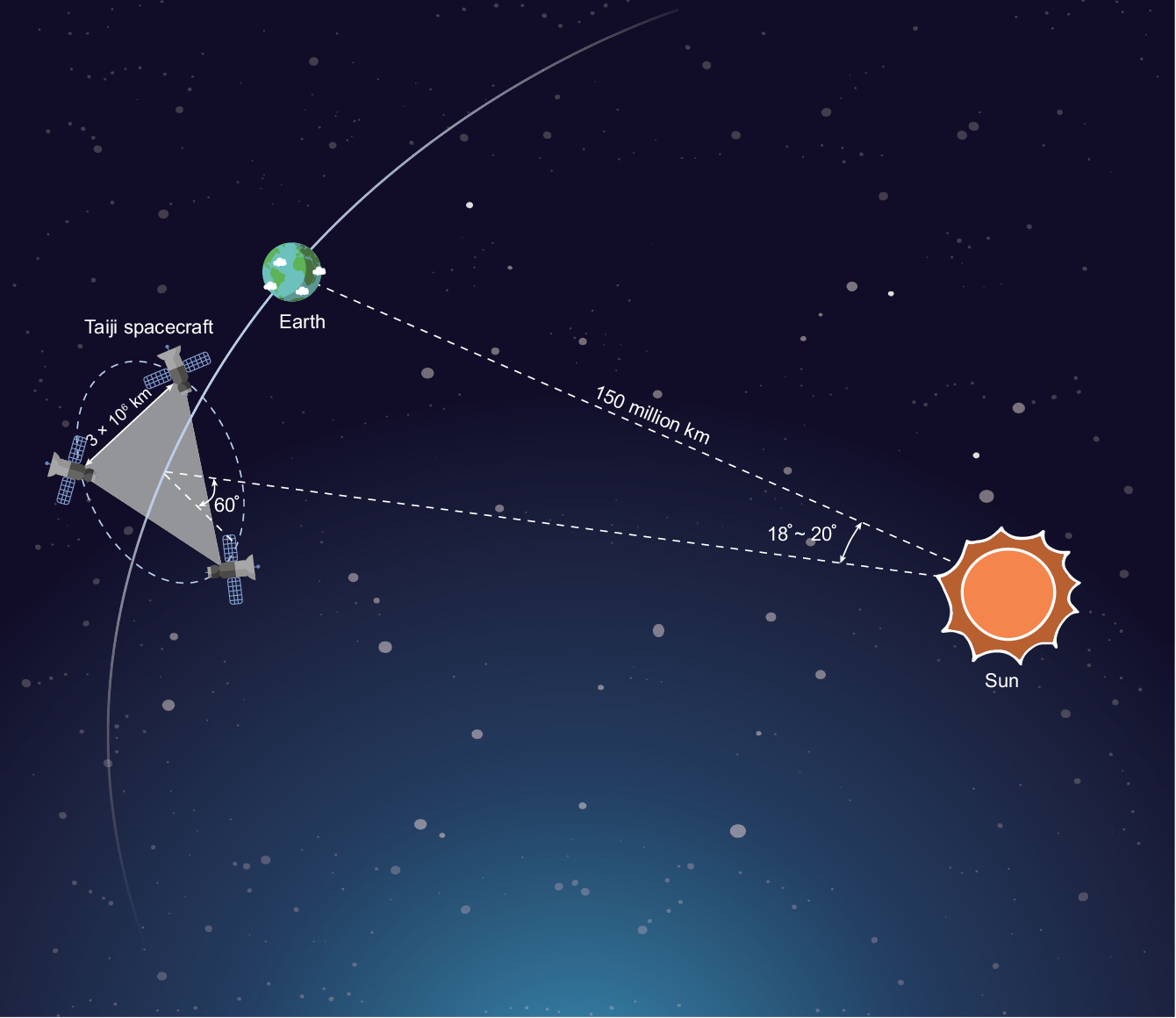
Taiji
Tianqin
https://twitter.com/chipro/status/1768388213008445837?s=46&t=JmDXWgIucgr_FlsBFTvuRQ
DINGO+SEOBNRv4EHM找了3个ebbh
Evidence for eccentricity in the population of binary black holes observed by LIGO-Virgo-KAGRA
https://dcc.ligo.org/LIGO-G2400750
BEFORE
AFTER
LIGO-G2300554
Content

- GW Astronomy
- AI for Science · GW Data Analysis
- GW search · Pipeline
- Parameter estimation · Scientific discovery
-
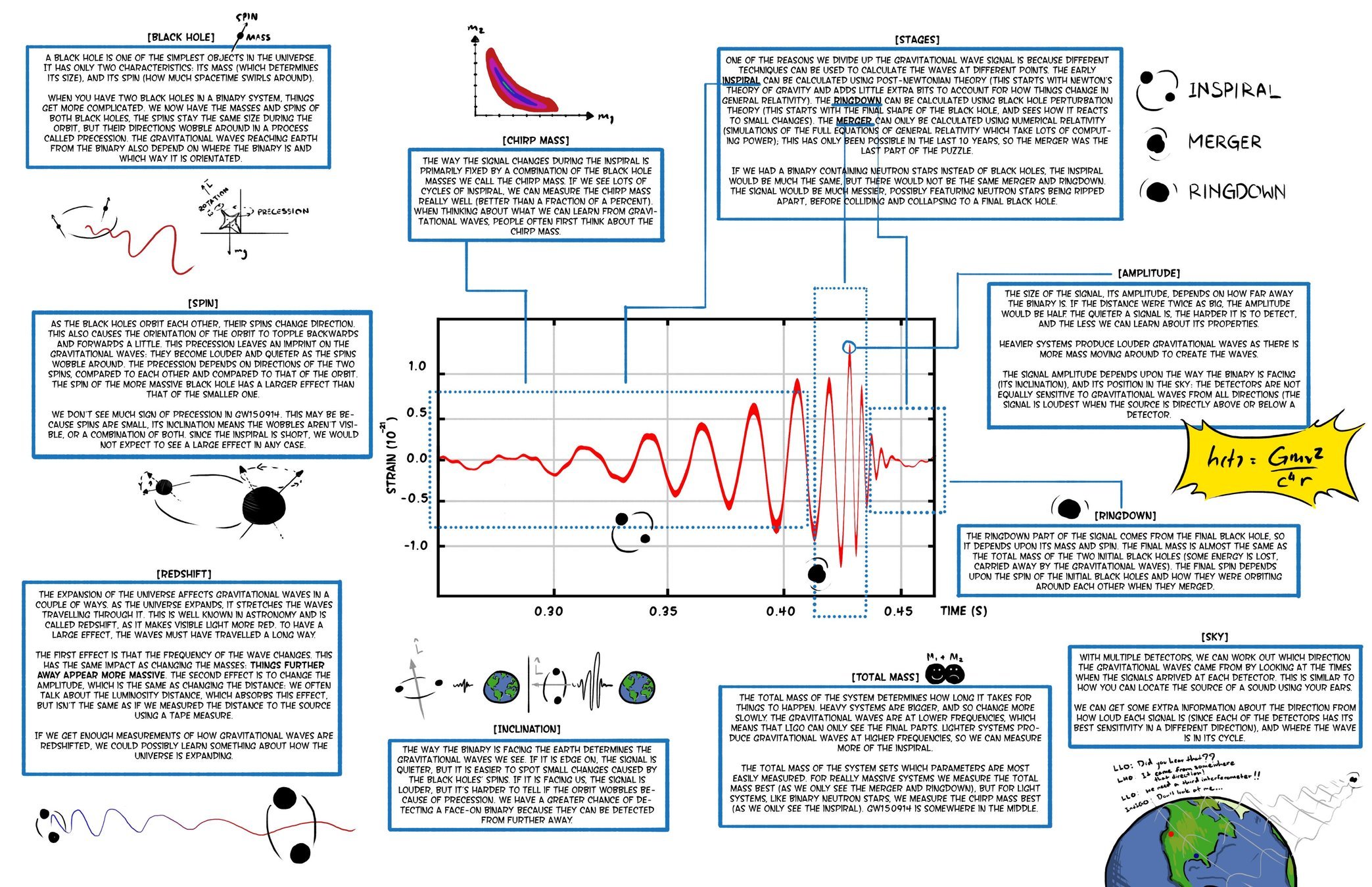
In 1916, A. Einstein proposed the GR and predicted the existence of GW.
-
Gravitational waves (GW) are a strong field effect in the GR.
-
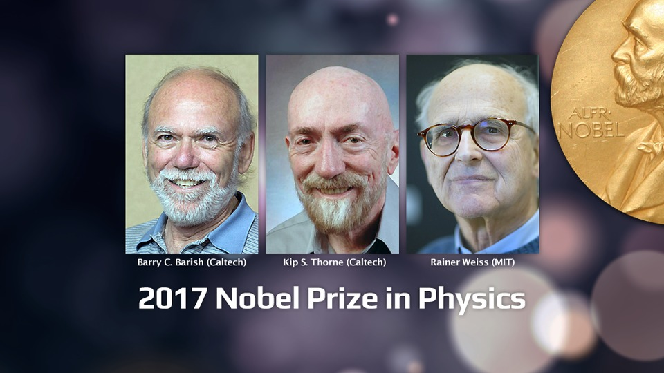
2015: the first experimental detection of GW from the merger of two black holes was achieved.
-
2017: the first multi-messenger detection of a BNS signal was achieved, marking the beginning of multi-messenger astronomy.
-
2017: the Nobel Prize in Physics was awarded for the detection of GW.
-
As of now: more than 90 gravitational wave events have been discovered.
-
O4, which began on May 24th 2023, is currently in progress.
-
Gravitational Wave Astronomy
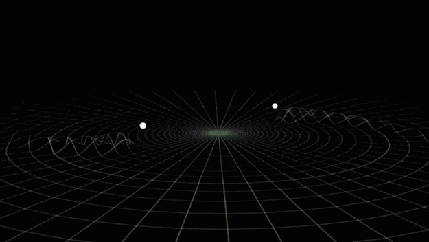

Gravitational waves generated by binary black holes system
GW detector
Gravitational Wave Astronomy
-
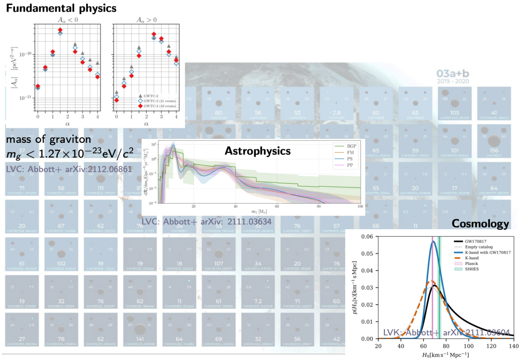
Fundamental Physics
- Existence of gravitational waves
- To put constraints on the properties of gravitons
-
Astrophysics
- Refine our understanding of stellar evolution
- and the behavior of matter under extreme conditions.
-
Cosmology
- The measurement of the Hubble constant
- Dark energy
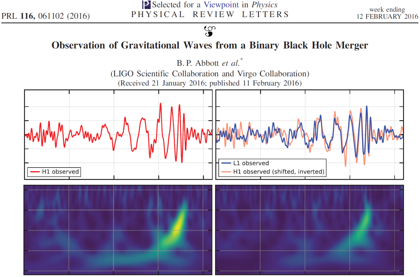
The first GW event of GW150914
Content
- WaveFormer: Transformer-Based Denoising Method for Gravitational-Wave Data
- Advancing Space-Based Gravitational Wave Astronomy: Rapid Detection and Parameter Estimation Using Normalizing Flows.
- Overview and Outlook
- Summary & Review
- Ongoing & Future Plan

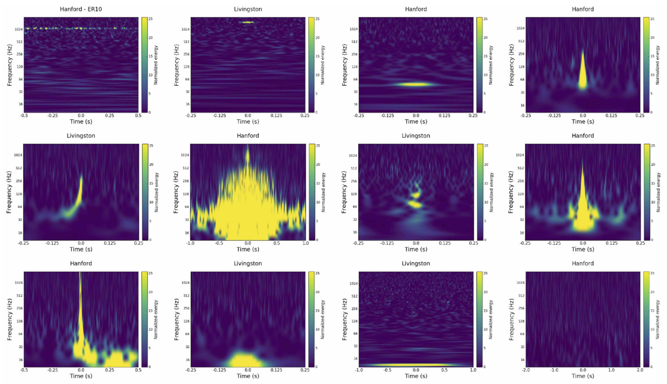
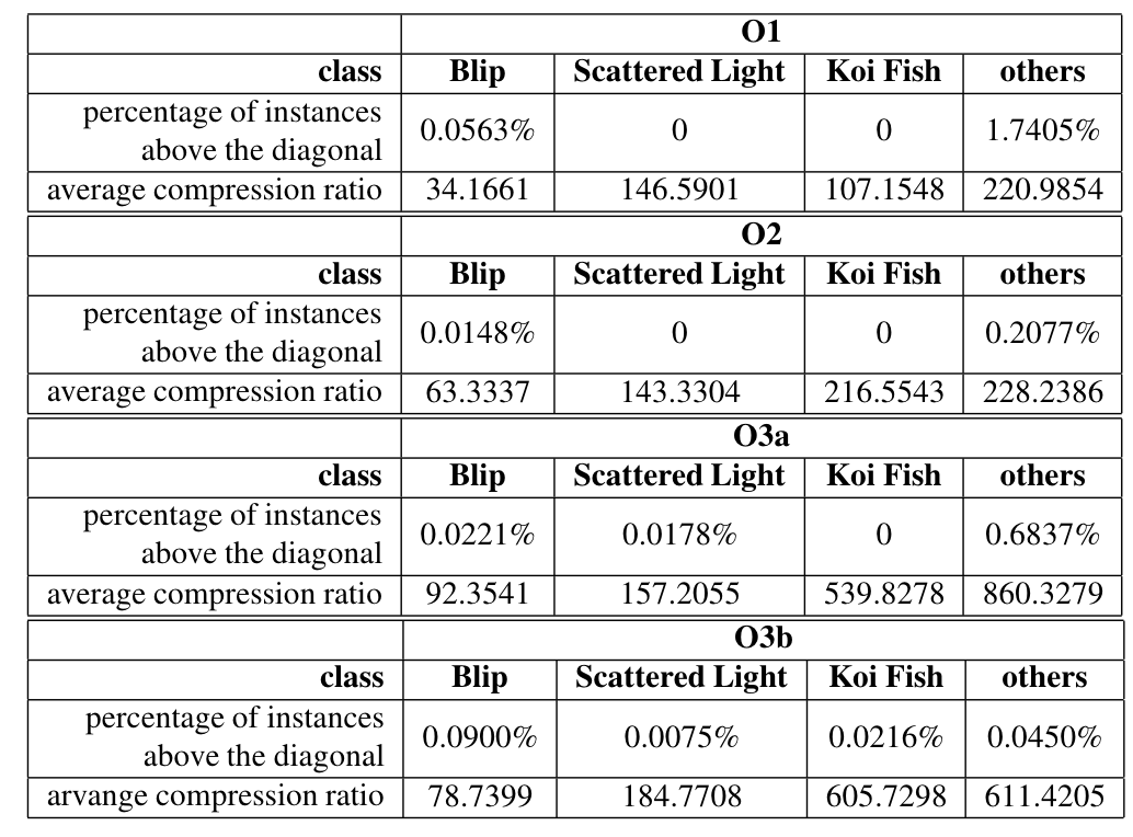
1400Ripples Air Compressor Blip
Extremely Loud Helix Koi Fish
Various types of Glitch
Background
-
The improvement of data quality is a very complex issue, with data from over 20,000 sensor channels determining the quality of the gravitational wave science data channel.
-
Reducing non-Gaussian short-duration pulse interference (Glitches) in gravitational wave data will help reduce the false alarm rate of gravitational wave signals.
-
Removing Glitches from gravitational wave detection data is a multi-classification problem.
- Traditional machine learning algorithms Powell J, et al. CQG, 2015
- Deep learning algorithms Zevin, M, et al. C
Ormiston R, et al. PRR, 2020
-
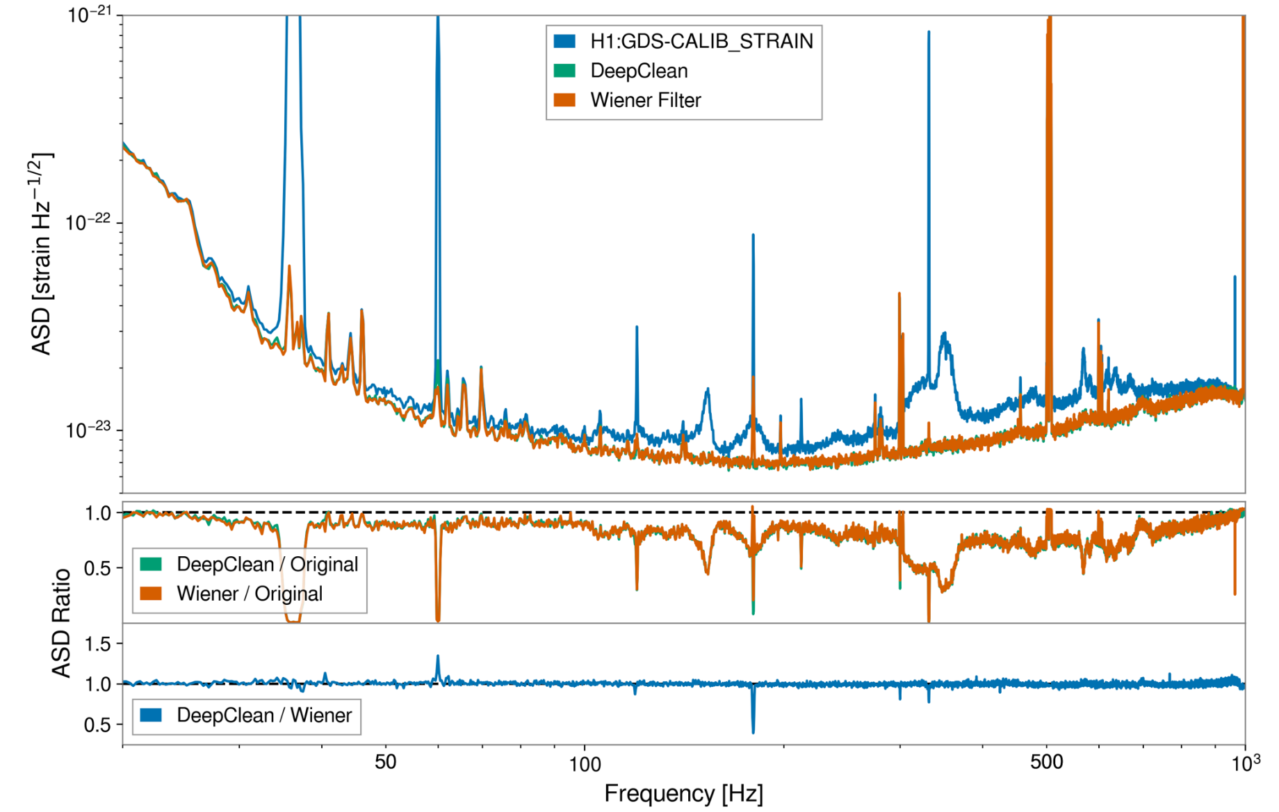
DeepClean: One-dimensional Convolutional Neural Network which takes a specified set of witness channels and subsequently outputs the predicted noise in strain.
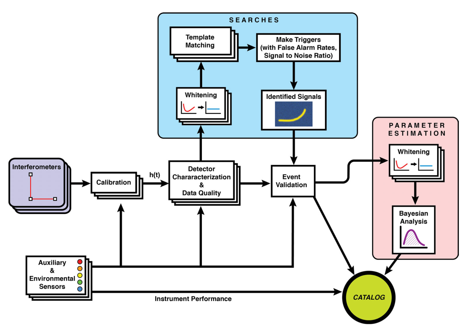
IGWN data processing
Non-stationary
Non-Gaussianity
Background
Related Works
Model Structure
Precessing & Train
Effect on Noise
Effect on BBH signals
Related Works
-
Extraction and denoising GW signals using deep learning:
- Both Wei et al. [PLB 2020] and Chatterjee et al. [PRD 2021] have shown that considering phase overlaps yields excellent results.
-
Detecting and denoising GW signals using deep learning:
- Both Bacon et al. [2205.13513] and Murali et al. [PRD 2023] could recover the phase of original GW signal with certain cycles but failed to recover the complete evaluation in amplitude scale.
Chatterjee C, Wen L, et al. PRD 2021
Wei W and Huerta E A. PLB 2020
Bacon P. et al. arXiv: 2205.13513
GW170823
Murali C & Lumley D. PRD 2023
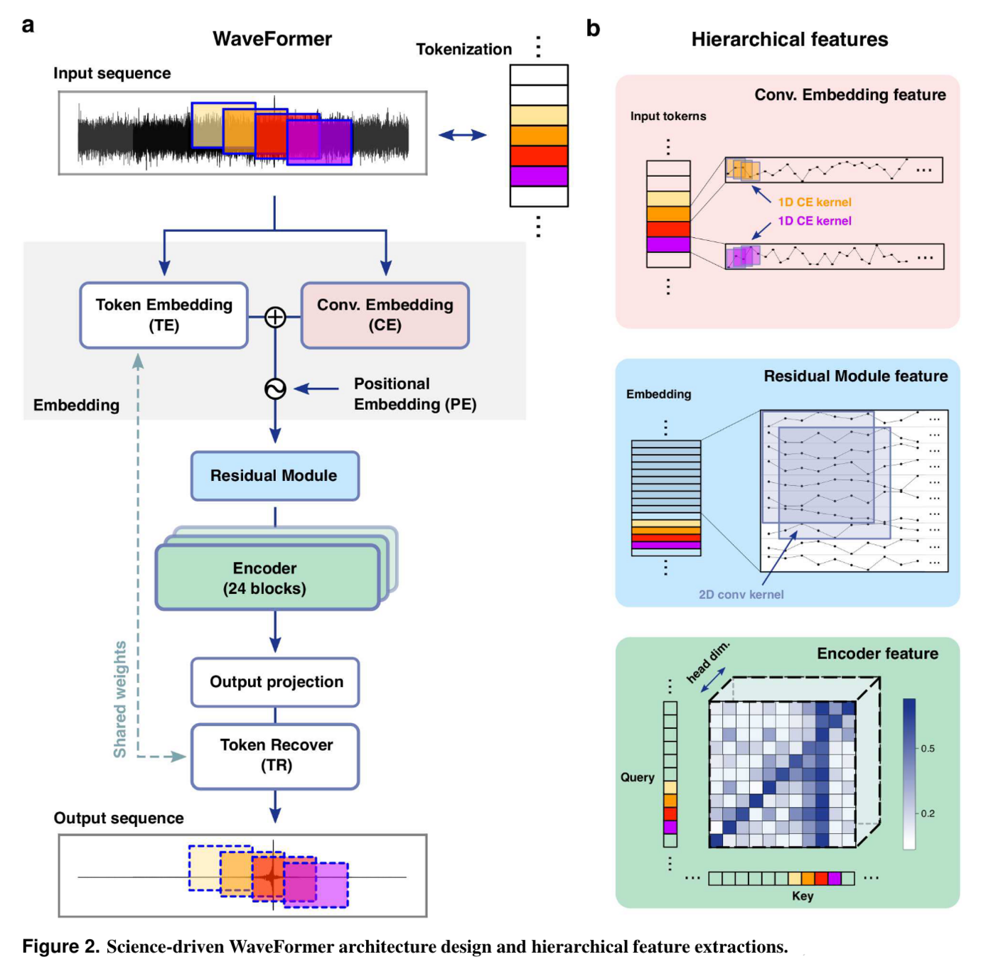
Network Architecture
- The WaveFormer, a billion-scale transformer-based model, excels in suppressing realistic noise and recovering injections or GW events, thereby significantly improving data quality.
- In its application, it treats each overlapping time-domain data subsequence as an individual token, akin to tokenization in natural language processing (NLP).


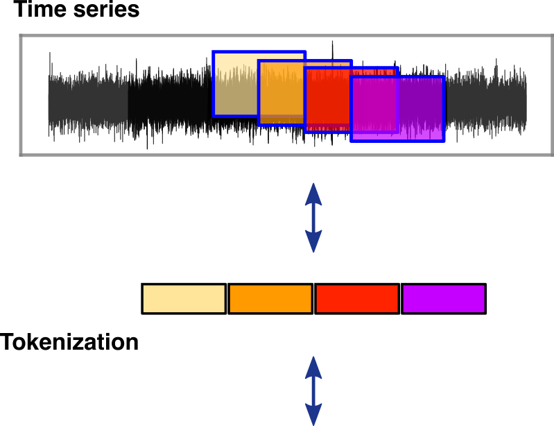
["This", "is", "a", "sample"]
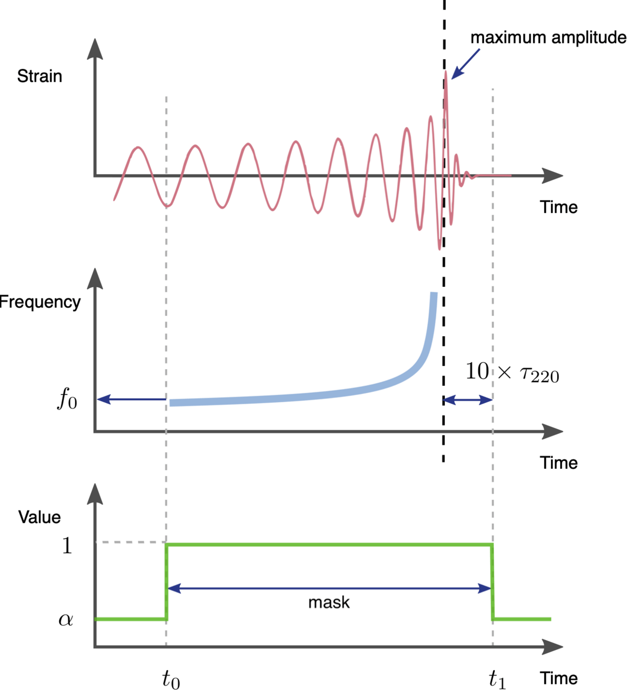
Data Preprocessing and Training Strategy
Strain
Whiten
Normalized
∼\(10^{−19}\)
∼\(10^{2}\)
∼\(10^{0}\)
32 s
32 s
merger
\(t_c\) (around GW150914)
(Cal network SNR)
Band-pass: [20, 2048] Hz
Patching (tokenized) with size 0.125 s and overlap 50%
[1, 128, 256]
(Standard normalization)
dynamic masking
[1, 16512]
[1, 128, 256]
(PSD\(_i\) from noise)
Band-pass: [20, 2048] Hz
WaveFormer
MSE-Loss\(_i\)
\(std\)
[1, 128, 256]
Noise\(_i\):
Signal\(_i\):
Input\(_i\):
Label\(_i\):
Output\(_i\):
8.0625 s
8.0625 s
Given �=ℎ+�d=h+n, we can normalize �d as follows:
-
Implementations:
- PSD sampling from real noise.
- input size: 8.0625 sec
- fs = 2048Hz
- Band-pass: 20~2048Hz
- Masked loss
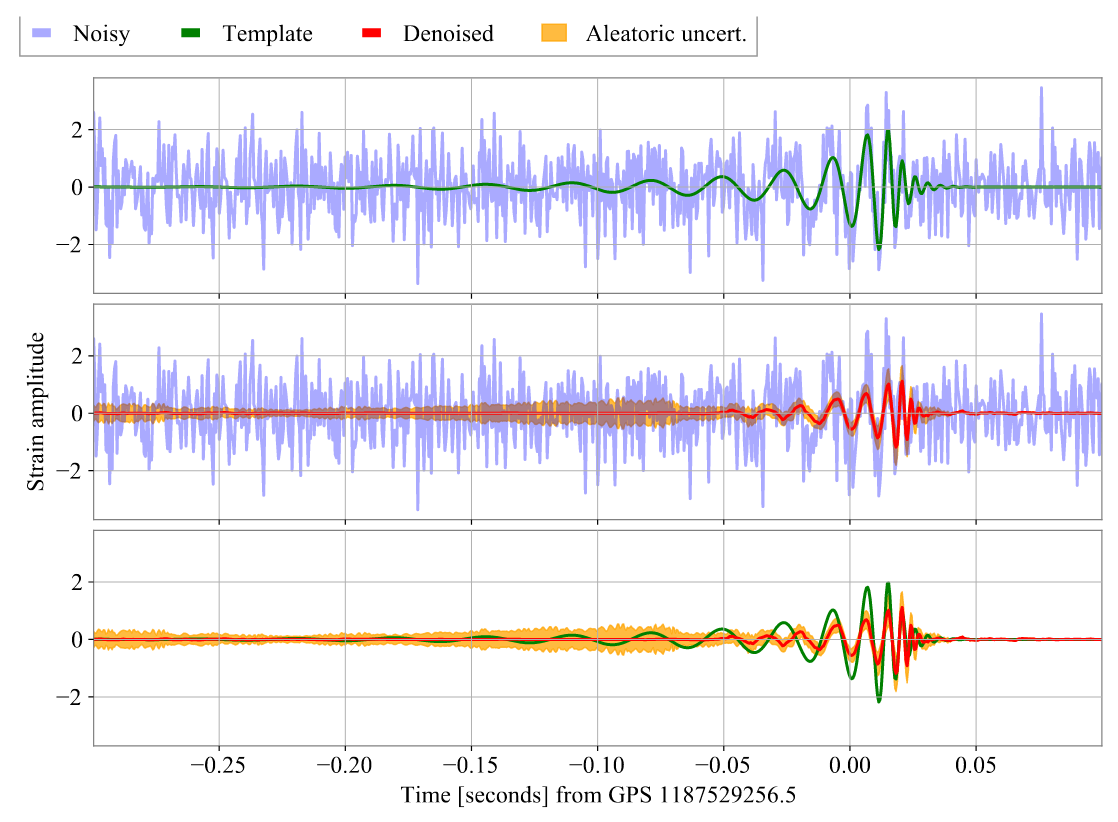
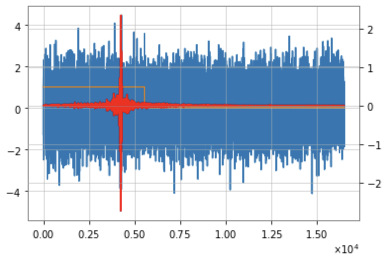
Effect on Realistic Noise
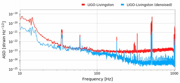
- Noise level percentile amplitude is significantly reduced, by approximately two orders.
- Further ASD analysis shows that WaveFormer effectively eliminates both narrowband and broadband spectral information, substantially lowering frequency contributions.
- Using the Gravity Spy database for glitches with SNR > 10 and confidence > 0.95, results show significant suppression of glitches in real advanced LIGO-Virgo noise.
(Bottom panels: results of glitches)
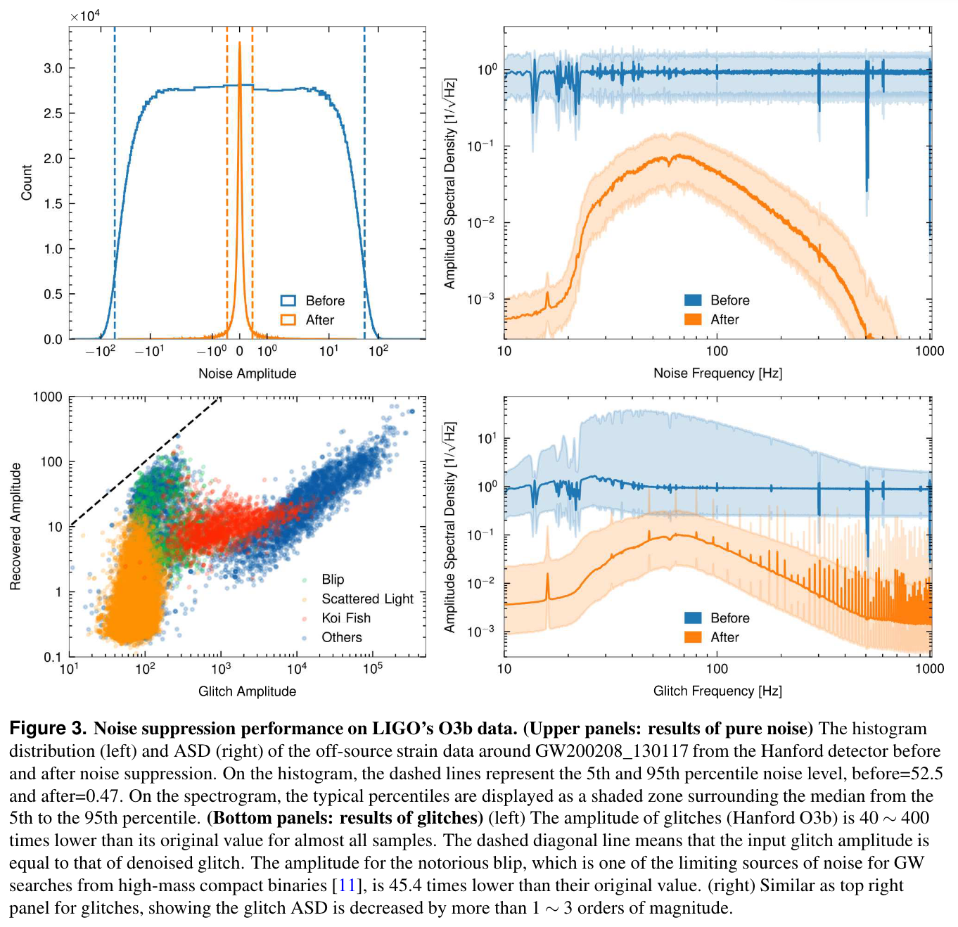
(Upper panels: results of pure noise)
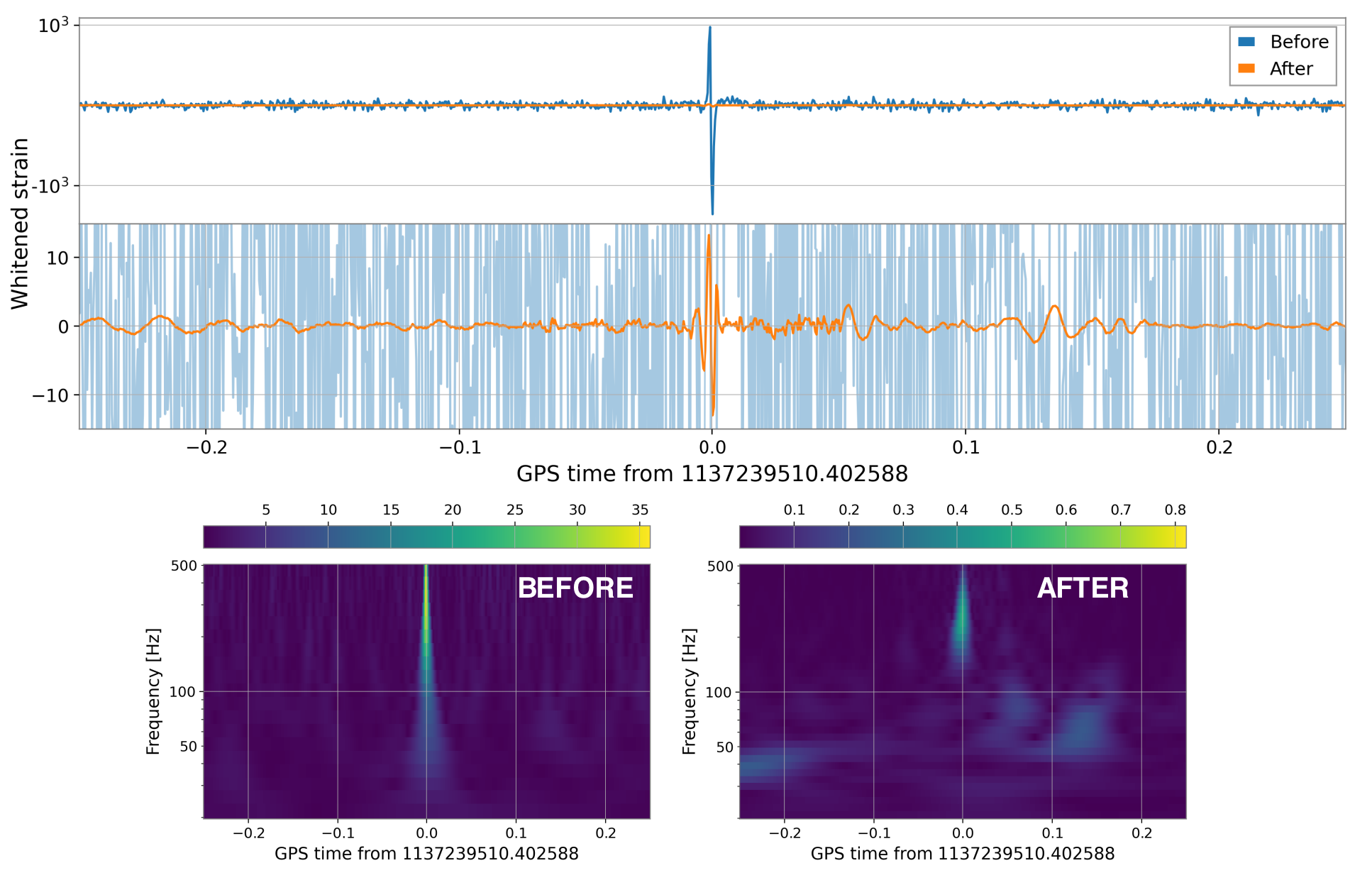
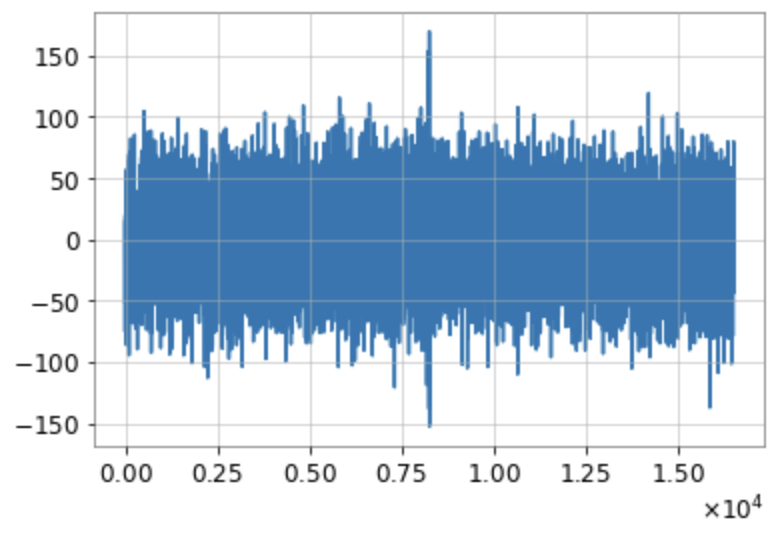
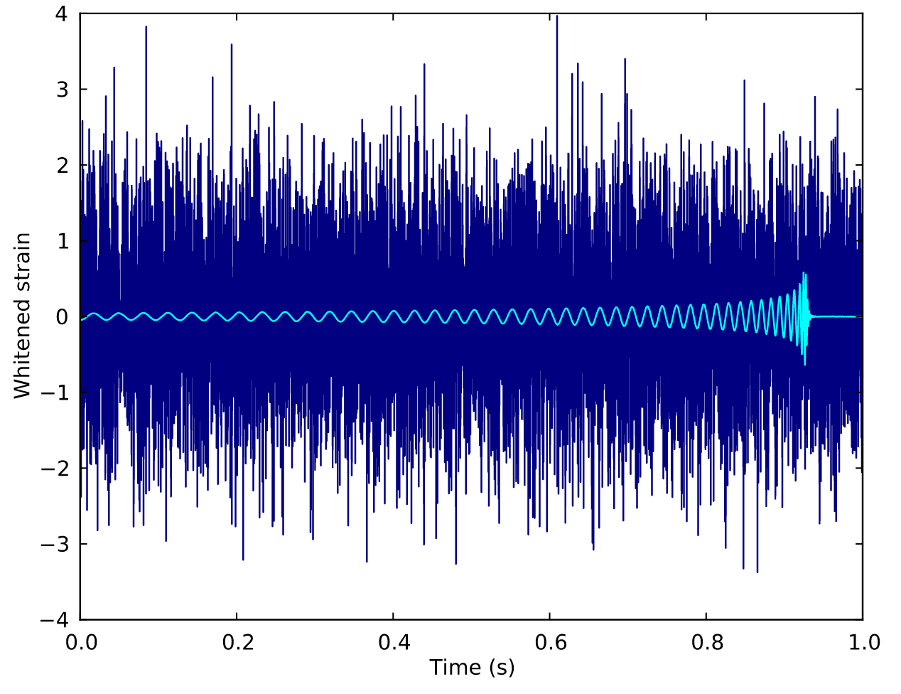
Time-series and spectrogram example of blip.

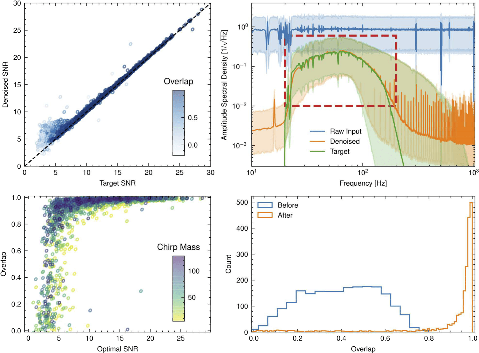
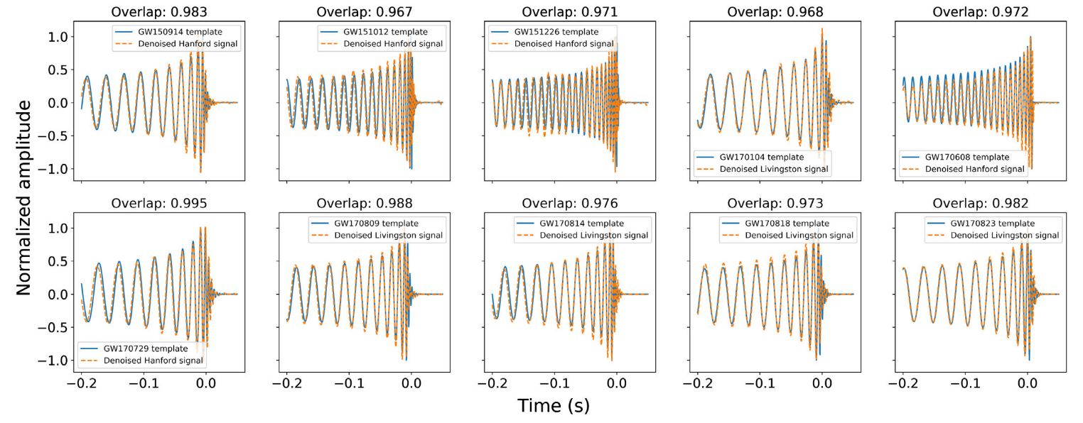
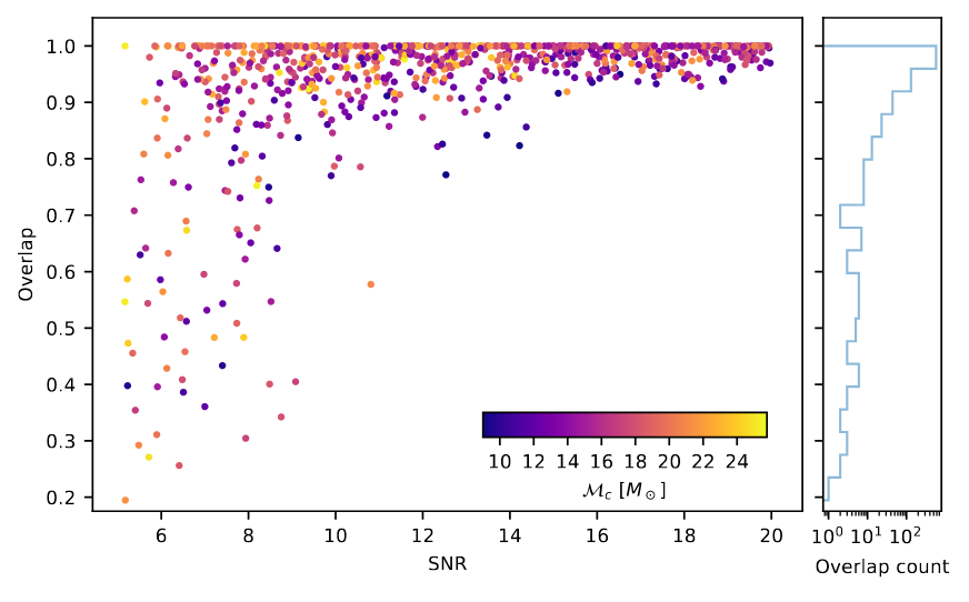
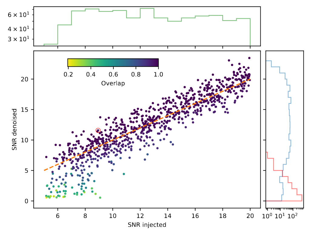
Recovery of Binary Black Holes
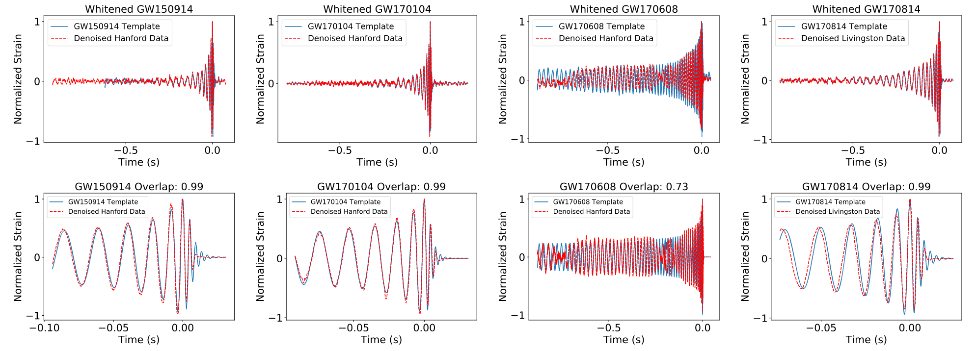
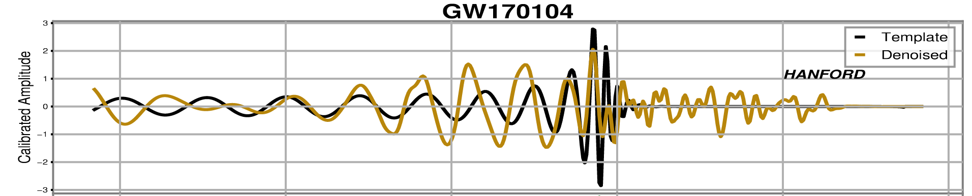
- Overlap and matched-filtering signal-to-noise are calculated to represent phase and amplitude recovery performance.
- Among the intermediate frequency range (20–200 Hz) that covers rich BBH signal information, the ASD distribution of denoised waveform is evidently consistent with that of target signal.
(Upper panels: Signal amplitude recovery performance
(Bottom panels: Signal phase recovery performance)
Bacon P. et al. arXiv: 2205.13513
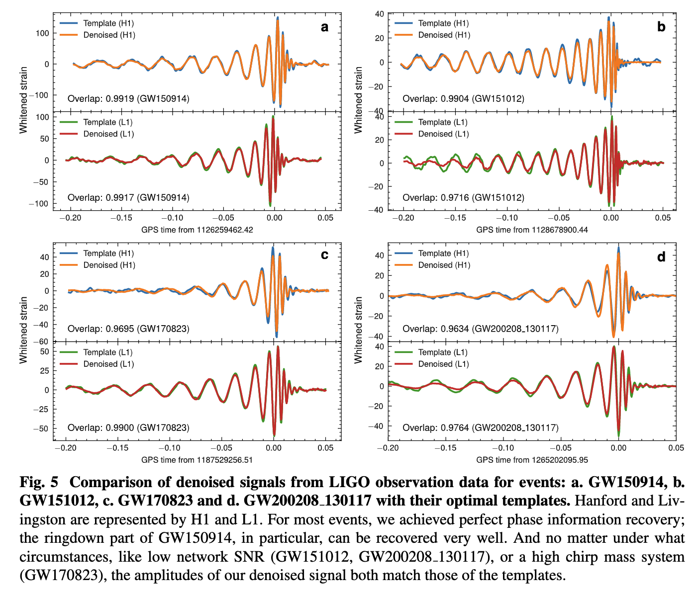
- These results show that our denoising algorithm outperformed others by capturing the characteristic chirping morphology of BBH evolution, and can denoise signals in realistic detection scenarios without affecting signal characteristics such as phase and amplitude.
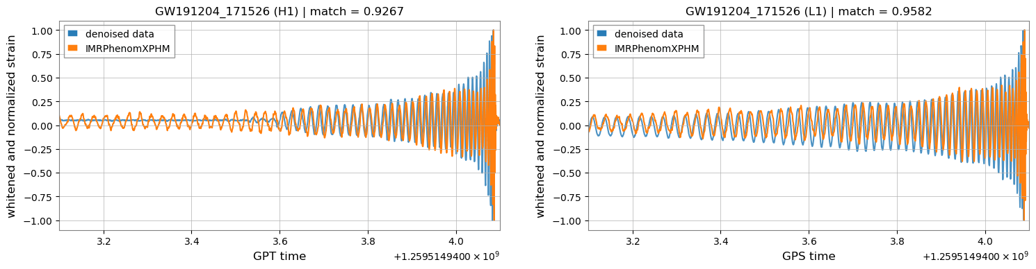
- For the event GW191204_171526, classified as either an NSBH or a low-mass BBH candidate in GWTC-3, the overlap with IMRPhenomXPHM achieved 0.93 and 0.95 on H1 and L1, respectively, which are marked improvements over those achieved by BayesWave and cWB (with overlaps between 0.82–0.86).
GW191204_171526
Recovery of Binary Black Holes
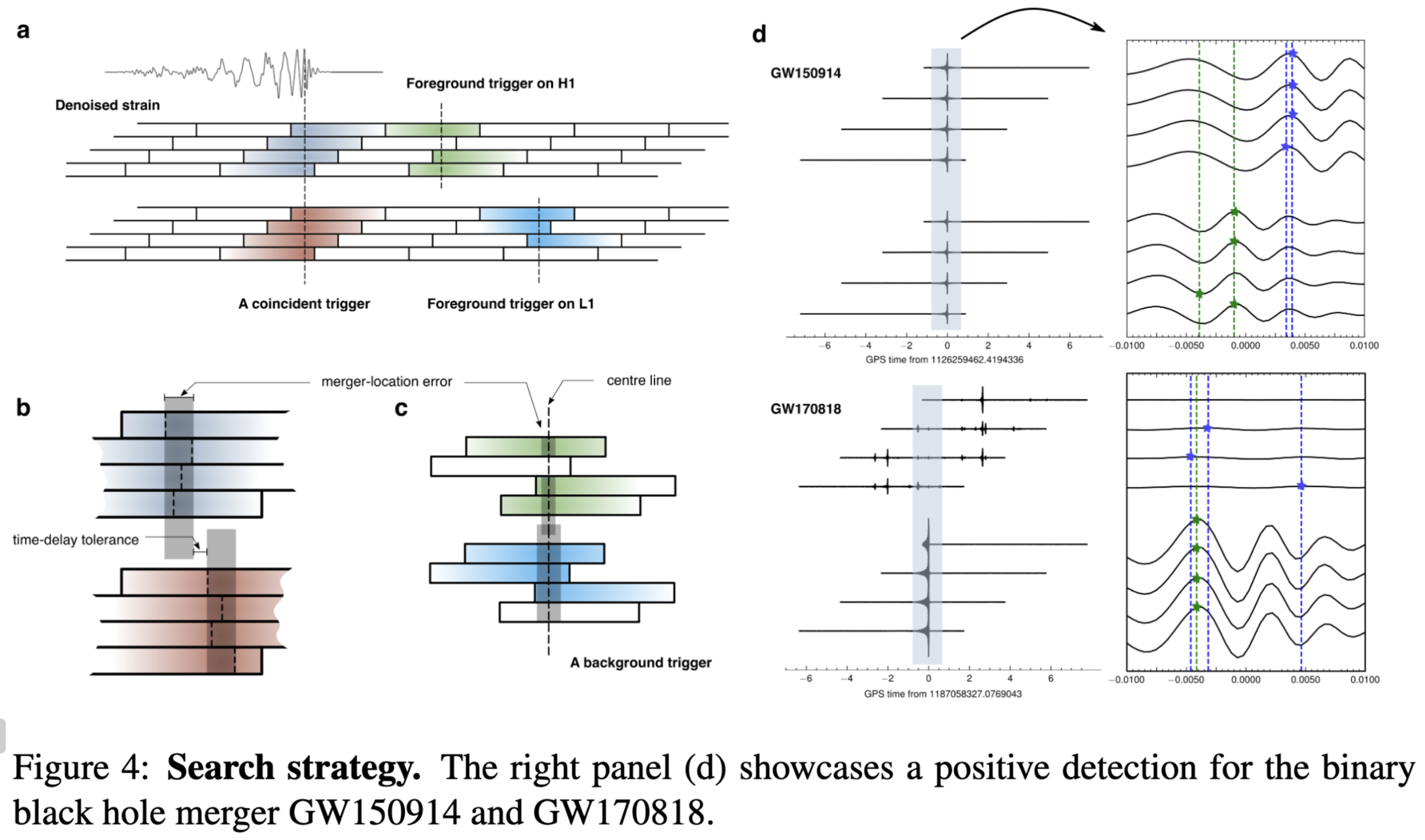
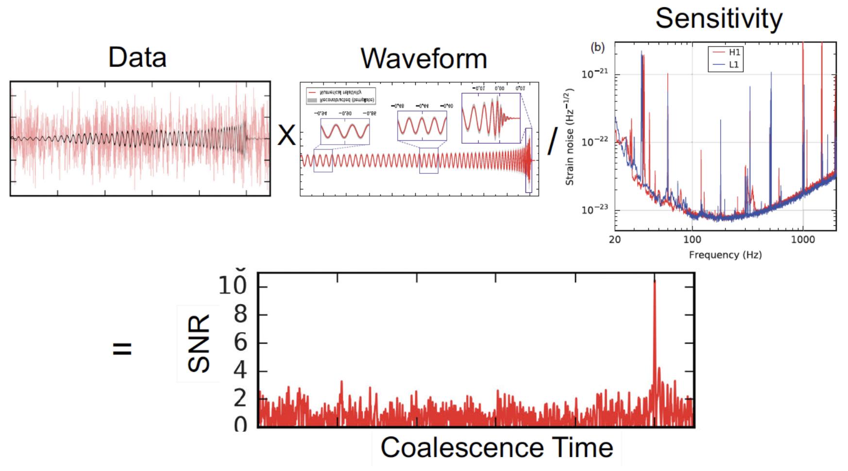
Search Strategy Overview
-
Firstly, we obtain the denoised output by utilizing Waveformer.
Then, triggers are defined and identified by three steps including:-
Find Peaks. Locate triggers on a single detector by finding its maximum all local-maximum (0.2s away from neighboring maximum/local-maximum).
-
By constraining triggers that exist on both two detectors, we get VALID triggers. (consist 3~4 segments)
-
Calculate the cross-correlation of the to-be-evaluated trigger across channels or within a single channel, between its noisy and corresponding denoised segments, as well as between denoised segments themselves.
-
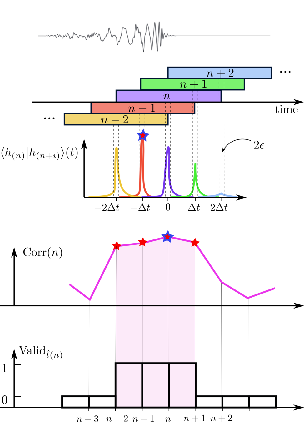
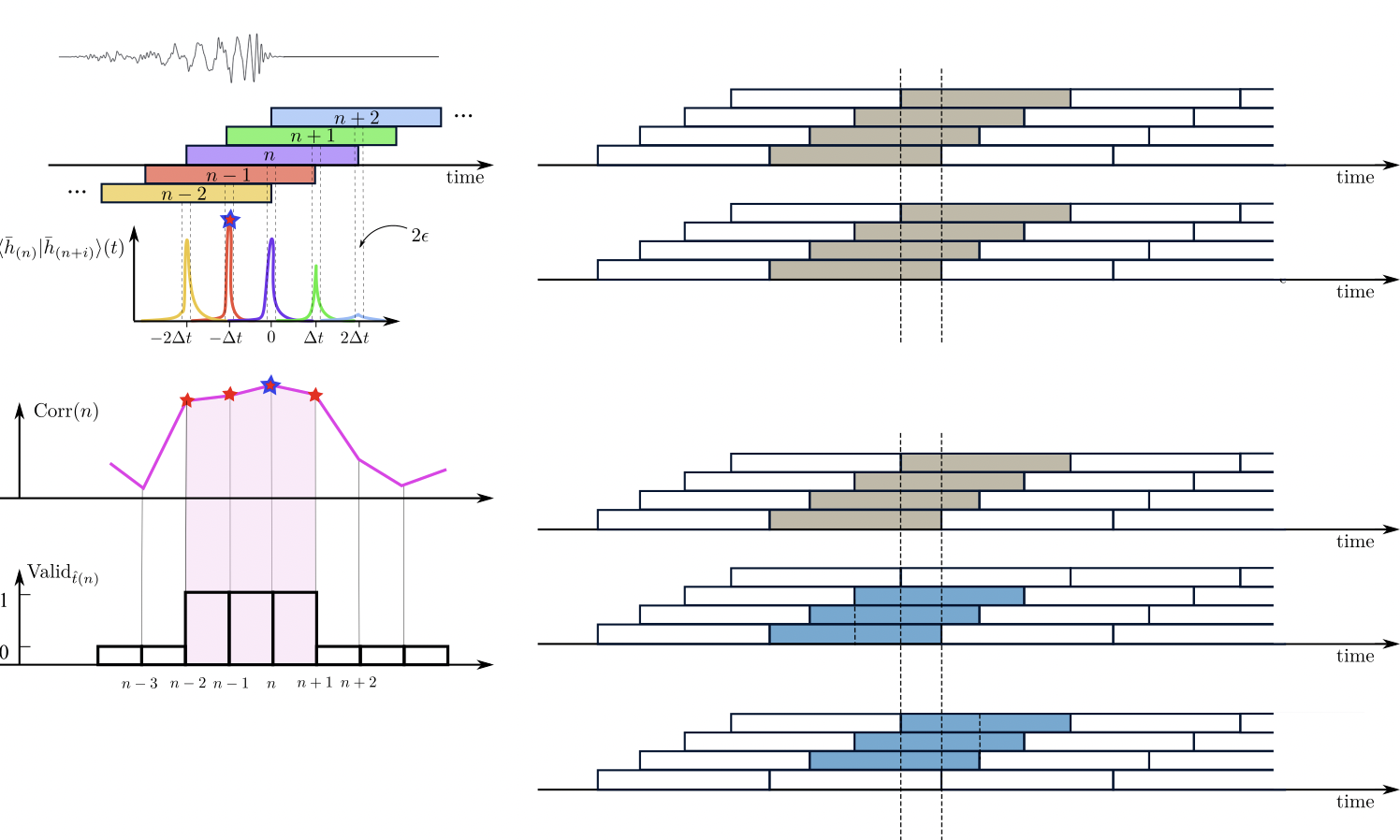
noisy input segments
denoised output segments
\(\bar{H}\)
\(\bar{L}\)
\({H}\)
\({L}\)
AI
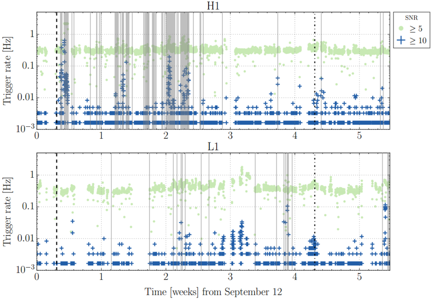
Significance Estimates
-
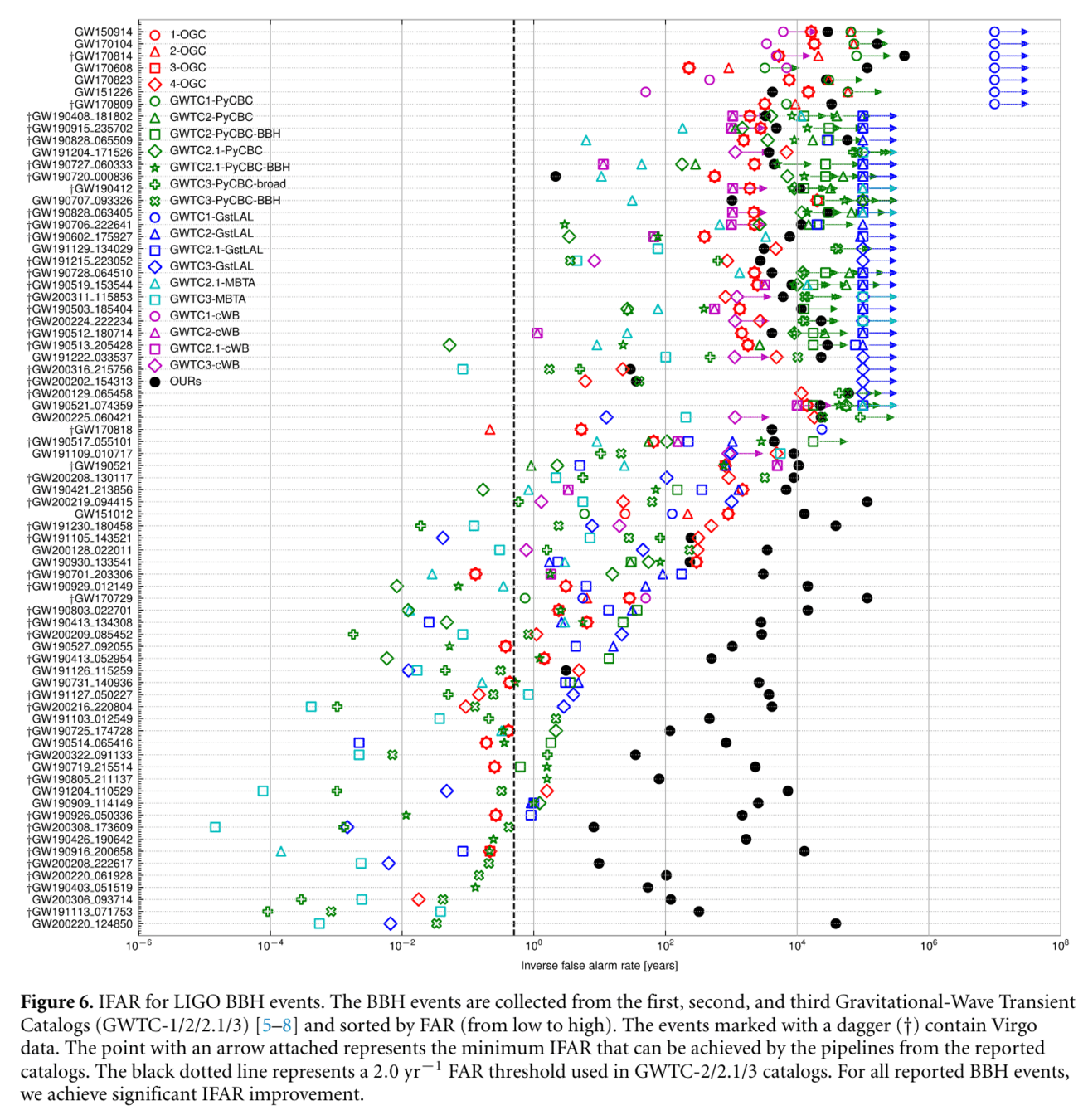
Assessed denoising workflow performance by comparing with GWTC-1, GWTC-2, GWTC2.1, and GWTC-3 catalogs and associated data releases.
-
Noted significant divergence in IFAR distribution between our results and those from GWTC and OGC catalogs.
-
Achieved significant IFAR improvement across all 75 reported BBH events, indicating effective suppression of loud terrestrial noise.
-
Example: For low SNR (\(10.8_{-0.4}^{+0.3}\)) event GW200208_130117, obtained an IFAR of 8916 years, surpassing maximum IFAR of <4000 years in other catalogs.
-
-
Variability in IFAR improvement linked to the original data's noise nature, including its non-Gaussian, non-stationary characteristics, and different signal recognition strategies by pipelines.
-
IFAR performance significantly depends on the reduction of non-Gaussian noise near each event.
-
Events with substantial IFAR improvement had misleading non-Gaussian noise effectively eliminated.
-
Events where IFAR underperforms retained non-Gaussian characteristics, possibly due to WaveFormer's inherent systematic errors.
-
Summary & Discussion
- Developed an AI-based workflow with WaveFormer, combining convolutional neural network and transformer for effective GW noise suppression and hierarchical feature extraction across a wide frequency range.
- Achieved significant noise suppression and signal recovery performance improvements, including state-of-the-art results on real observational data and BBH events, leading to dramatic data quality improvement and significant IFAR enhancement on 75 reported BBH events.

Text
-
Challenges in Model Interpretability
- The black-box nature of AI models complicates interpretability, challenging the comparison of AI-generated detection statistics with traditional matched filtering chi-square distributions.
- Convincing the scientific community of the pipeline's validity and the statistical significance of new discoveries remains difficult despite the model's ability to identify potential gravitational wave signals.
He Wang, et al. MLST. 5, 1 (2024): 015046.
LVK. arXiv:1602.03839
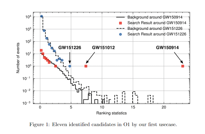
GW151226
GW151012
Content
- WaveFormer: Transformer-Based Denoising Method for Gravitational-Wave Data
- Advancing Space-Based Gravitational Wave Astronomy: Rapid Detection and Parameter Estimation Using Normalizing Flows.
- Overview and Outlook
- Summary & Review
- Ongoing & Future Plan
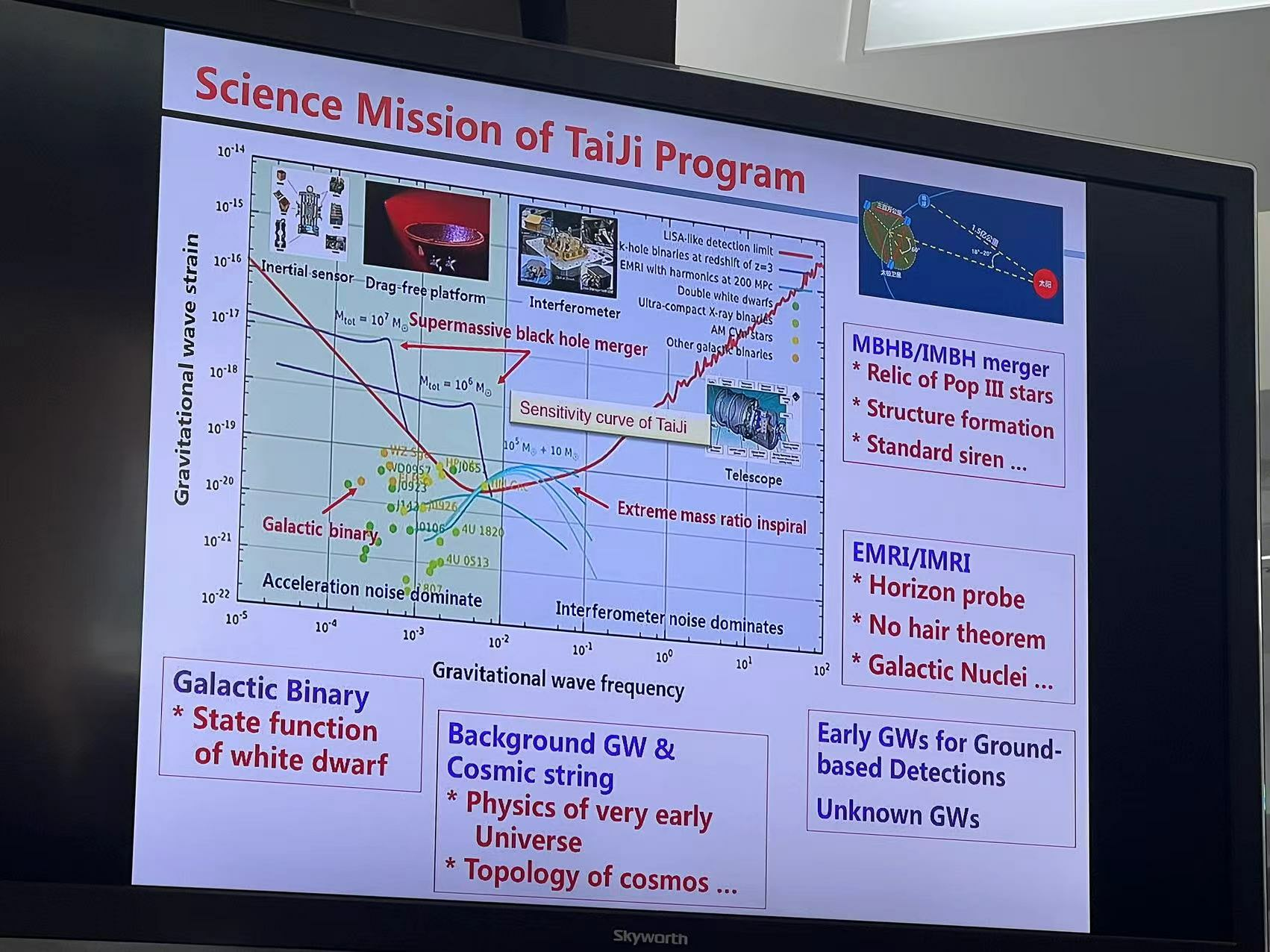
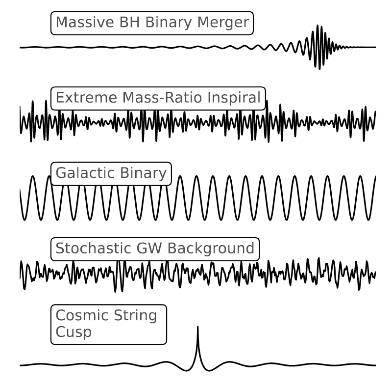
Gravitational waves and sources:
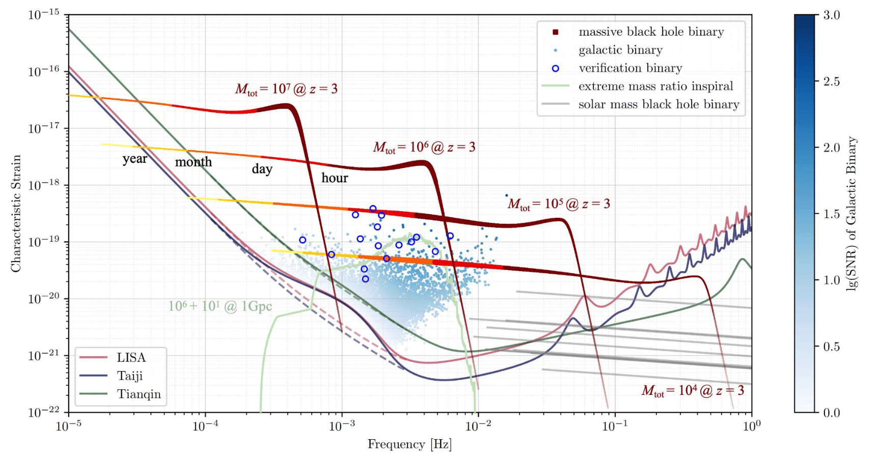
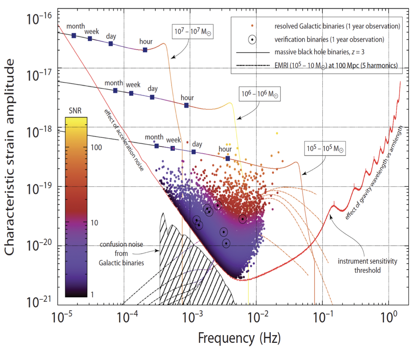
- Galactic Binary (GB) [\(\mathcal{O}(10^4) \text{ in } \mathcal{O}(10^7)\)]
- Massive Black Hole Binary (MBHB) [\(\mathcal{O}(2)\sim\mathcal{O}(10^2)\)]
- Extreme Mass-Ratio Inspiral (EMRI) [\(\mathcal{O}(10)\sim\mathcal{O}(10^3)\)]
- Stellar-mass Black Hole Binary (SBHB)
- Stochastic Gravitational Wave Background (SGWB)
- Unmodelled sources (eg: Burst...)
Wang H, Du M H, Xu P, Zhou Y F. Sci Sin-Phys Mech Astron, 2024, 54, doi: 10.1360/SSPMA-2024-0087
Credit: ESA, K. Holley-Bockelmann

(Sec.8.3.1 The Red Book)
The analysis of scientific data from space-based GW detection differs significantly from ground-based detection:
- A superposition of overlapping signals ( \(\neq\) isolated event)
- Observations of more waveform periods over different time scales ( \(\neq\) short-duration signals)
- Signal-dominated detection ( \(\neq\) noise-dominated)
- Reliance on more complex techniques for noise assessment
( \(\neq\) regular acquisition of signal-free data)
Space-borne GW Detection: Background
Space-borne GW Detection: Background
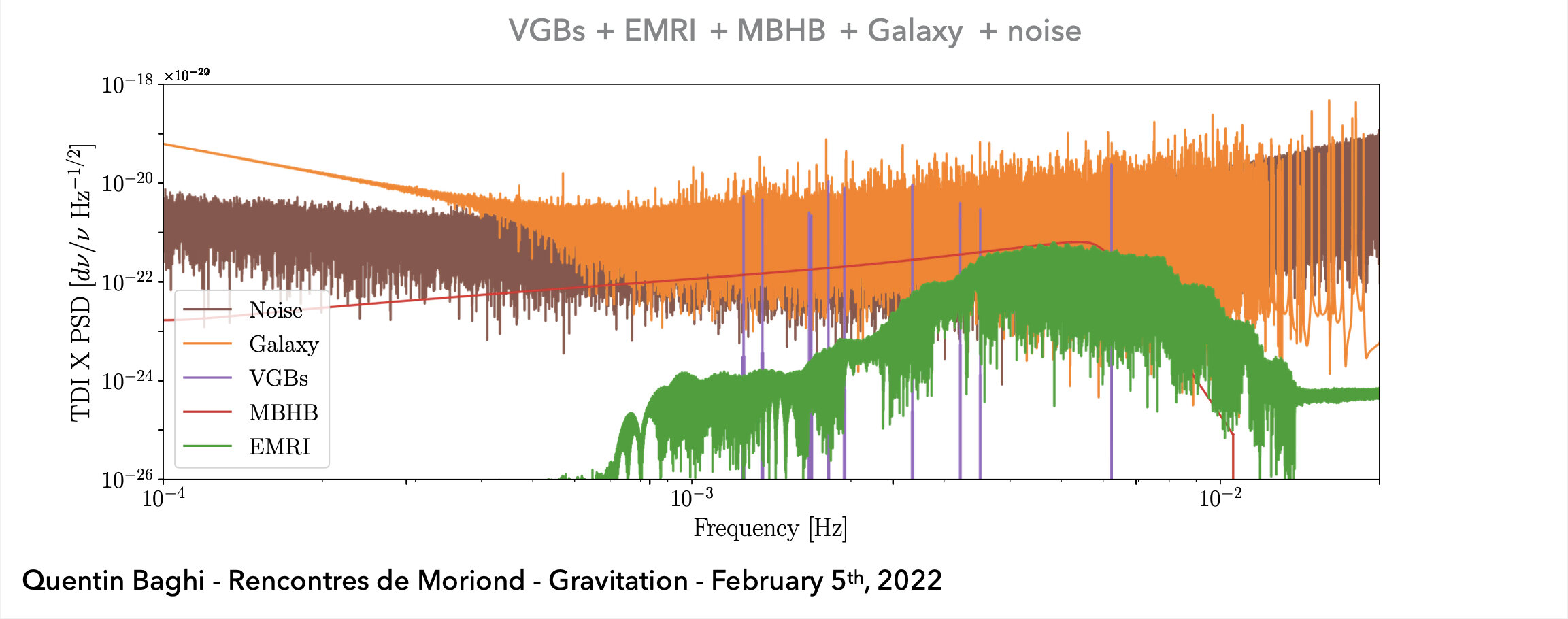
Analyses cannot treat sources independently and sequentially work through a list of candidate detections.
The analysis of scientific data from space-based GW detection differs significantly from ground-based detection:
- A superposition of overlapping signals ( \(\neq\) isolated event)
- Observations of more waveform periods over different time scales ( \(\neq\) short-duration signals)
- Signal-dominated detection ( \(\neq\) noise-dominated)
- Reliance on more complex techniques for noise assessment
( \(\neq\) regular acquisition of signal-free data)
- The data analyses depend on the simultaneous fitting of complete astrophysical, cosmological, and instrument models to the observed data.
- The need for this so-called “global fit” was identified as the primary challenge to the data analysis early in the space-borne mission formulation.
(Sec.8.6 The Red Book)
Rapid PE for Space-borne GW Detection
M. Du, B. Liang, HW, P. Xu, Z. Luo, Y. Wu. SCPMA 67, 230412 (2024).
-
Global vs. Individual Analysis: While global-fit techniques effectively manage the dense overlapping of signals in space-based GW data, individual pipelines are crucial for detecting unique events.
-
Role of Individual Pipelines: These pipelines act as a pre-processing step, focusing on particular types of sources and diving deeper into the data. They refine the analysis by working on the latest best-fit residuals from the global fit.
-
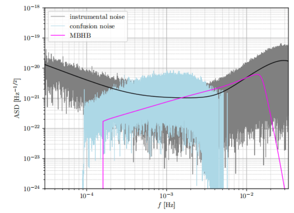
Case Study - MBHB Mergers: Mergers of MBHBs often exhibit high SNR between \(10^2\) to \(10^3\), appearing as distinct peaks in data time series.
-
Data curation
-
Model: frequency domain; PhenomD; TDI-A/E response
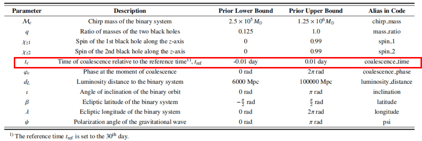
-
Input: 1 day length; 15Hz; shape=(2, 3, 2877)
-
Noise: Gaussian stationary from the noise PSD (for training/test) + GB confusion noise (for test)
-
Project: Taiji program
-
M. Du, B. Liang, HW, P. Xu, Z. Luo, Y. Wu. SCPMA 67, 230412 (2024).
Customization for the Taiji scenario: A scalable approach
-
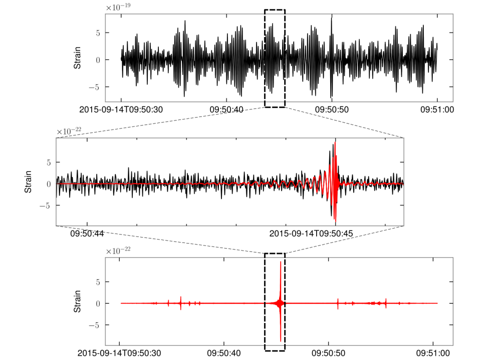
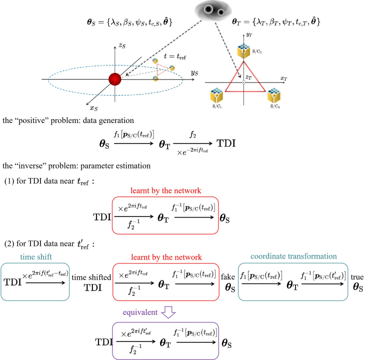
The top section of the illustration shows the solar system barycenter (SSB) and Taiji frames, with two black dashed arrows symbolizing not two separate GW signals, but rather indicating how the sky location and arrival time of the same GW signal take different values in these two frames.
-
The “positive” problem translates the SSB-frame parameters to their Taiji-frame counterparts via a time-dependent mapping \(f_1\), then to the TDI outputs through a time-independent mapping \(f_2\), and an exponential term.
TDI-A
-
These steps can be schematically summarized as:
where \(\mathcal{T}_\alpha^{A, E}(f)\) is often referred to as the transfer function.
M. Du, B. Liang, HW, P. Xu, Z. Luo, Y. Wu. SCPMA 67, 230412 (2024).
Customization for the Taiji scenario: A scalable approach
-
Consequently, even if the network has only learned the time-dependent relationship between \(\boldsymbol{\theta}_S\) and the TDI response at a specific tref (the 30th day in our case), with the aid of coordinate transformation, it has essentially learned the time-invariant mapping \(f_2\), and can be then generalized to make parameter estimation at any other reference time.
-
It is worth noting that our method relies on analytical orbits and
the time-independence of the coordinate transformation \(f_2\).
-
The top section of the illustration shows the solar system barycenter (SSB) and Taiji frames, with two black dashed arrows symbolizing not two separate GW signals, but rather indicating how the sky location and arrival time of the same GW signal take different values in these two frames.
-
The “positive” problem translates the SSB-frame parameters to their Taiji-frame counterparts via a time-dependent mapping \(f_1\), then to the TDI outputs through a time-independent mapping \(f_2\), and an exponential term.
M. Du, B. Liang, HW, P. Xu, Z. Luo, Y. Wu. SCPMA 67, 230412 (2024).
Unbiased estimation and confidence validation
-
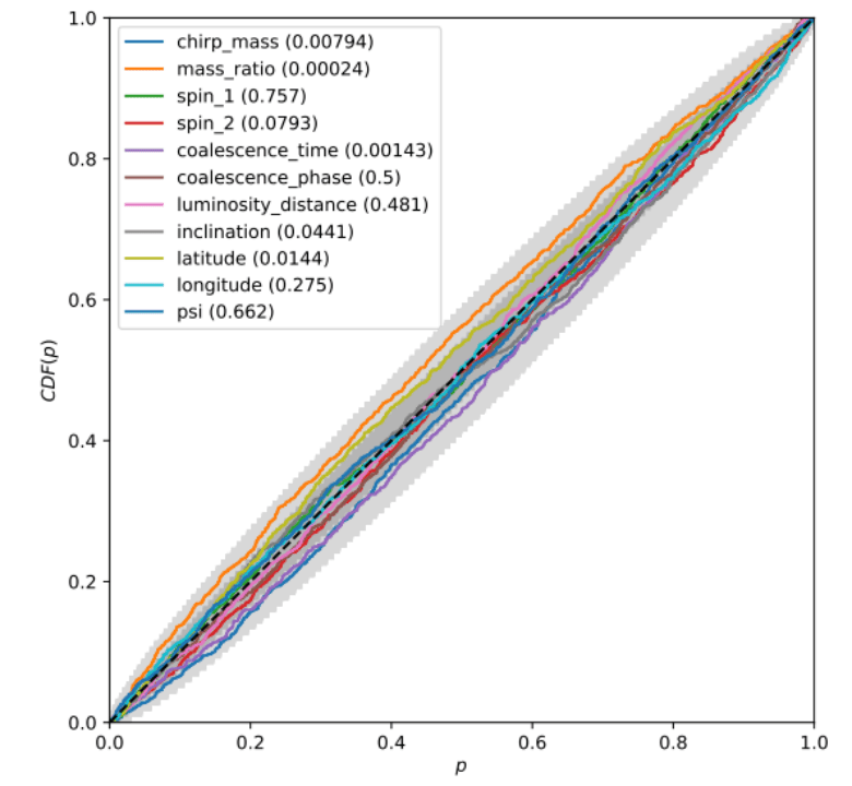
Methodology: Utilization of the Kolmogorov-Smirnov (KS) test to compare one-dimensional distributions generated by our algorithms, ensuring the accuracy of parameter estimation.
-
Empirical Validation: Conducted extensive testing on simulated signals, injecting 1000 waveforms from the prior with added confusion noise and varying reference times between 1 and 365 days.
-
Results: The tests assessed the frequency at which true parameters fell within certain confidence levels, confirming that our credible intervals are well-calibrated and reflect true confidence in the signal parameters.
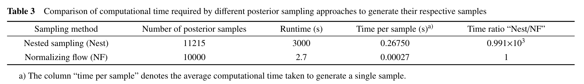
Computational performance
-
10000 posterior samples in 2.7 sec
- The remarkable speed of our method, which outpaces traditional techniques by several orders of magnitude, establishes it as an invaluable tool for preprocessing in global fitting.
M. Du, B. Liang, HW, P. Xu, Z. Luo, Y. Wu. SCPMA 67, 230412 (2024).
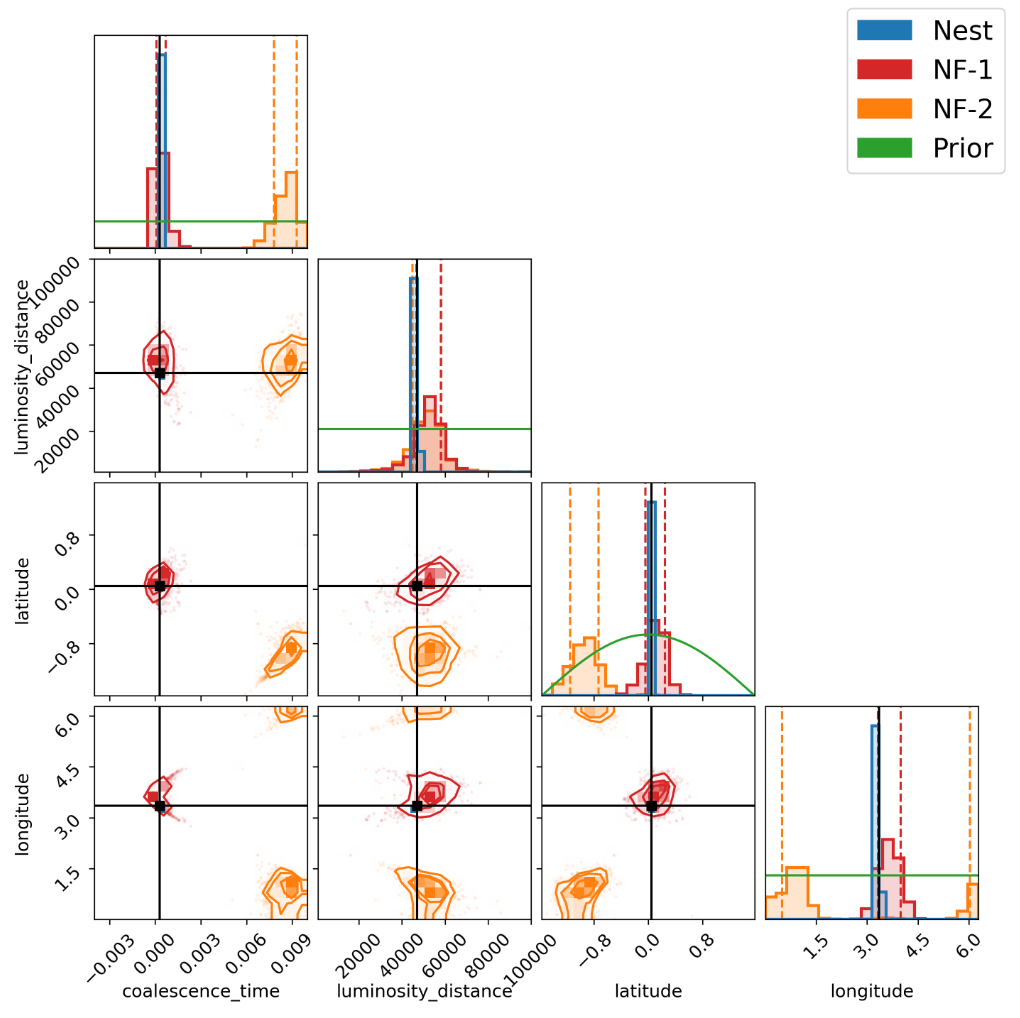
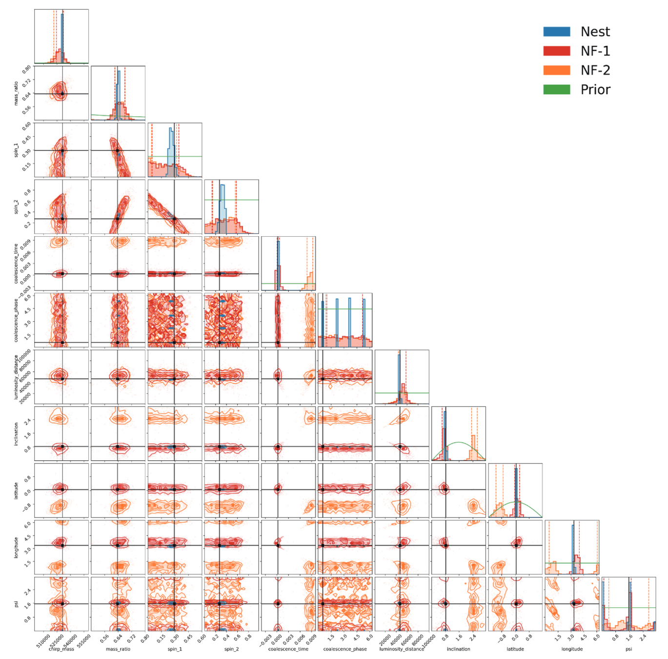
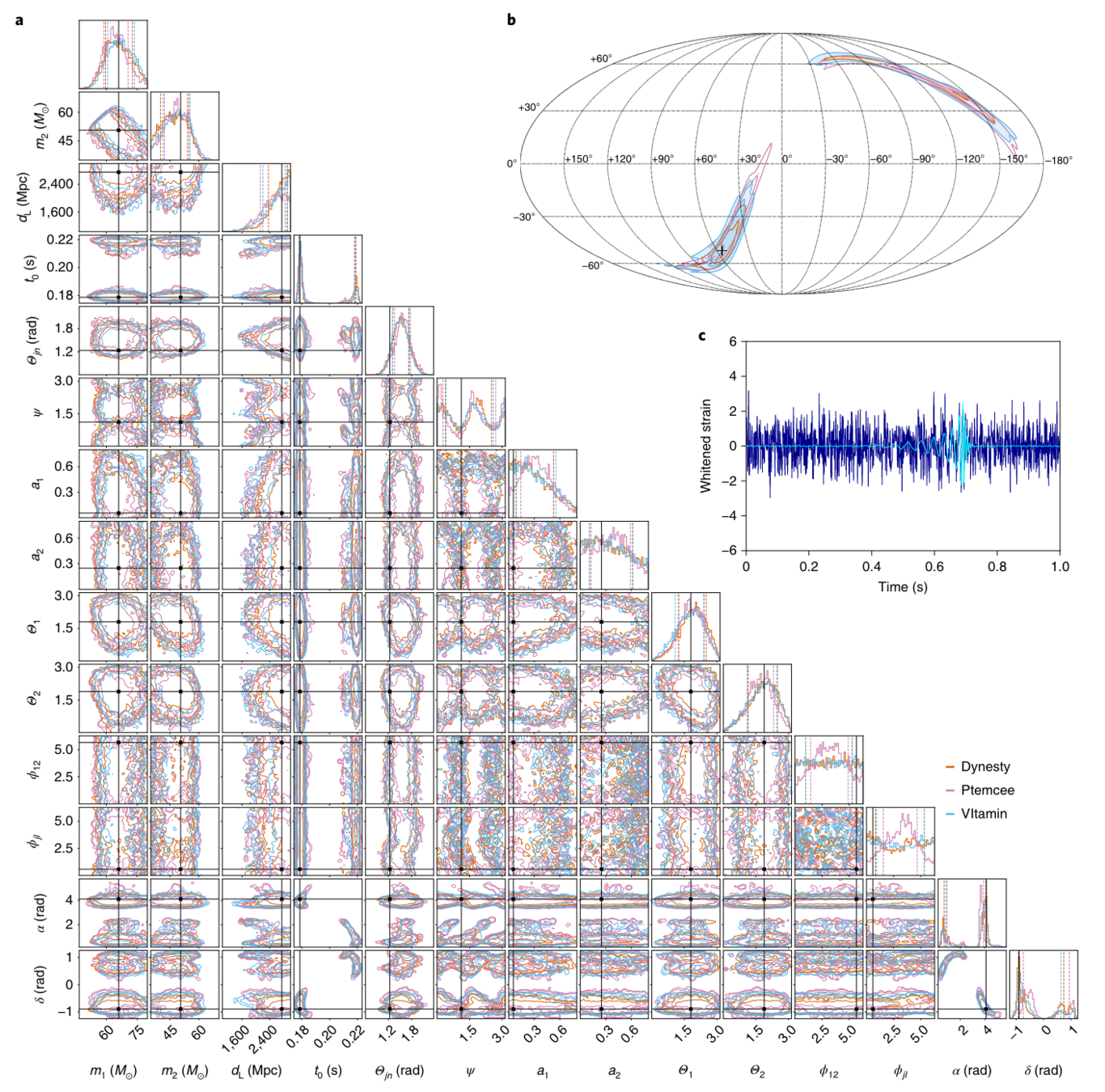
Multimodality in extrinsic parameters
-
Overview of Findings: Nested sampling results indicate minimal expected multimodality in ecliptic coordinates. However, distinct peaks identified in the time of coalescence (\(t_c\)), labeled as NF-1 (dominant) and NF-2 (subdominant), highlight unique multimodal behavior.
- Impact on PE: The presence of these peaks affects the posterior distributions of extrinsic parameters, potentially leading to inaccuracies in \(t_c\) and subsequent parameters due to phase term associations and inherent degeneracies.
- Model Performance: Despite the multimodality, the best-fit values from the NF model closely align with true values within the \(1\sigma\) range for most parameters, and at least \(2\sigma\) for others.
- Comparative Analysis: The ML pipeline tends to produce broader posteriors compared to the Bayesian nested sampling approach.
(NF = Normalizing Flow model)
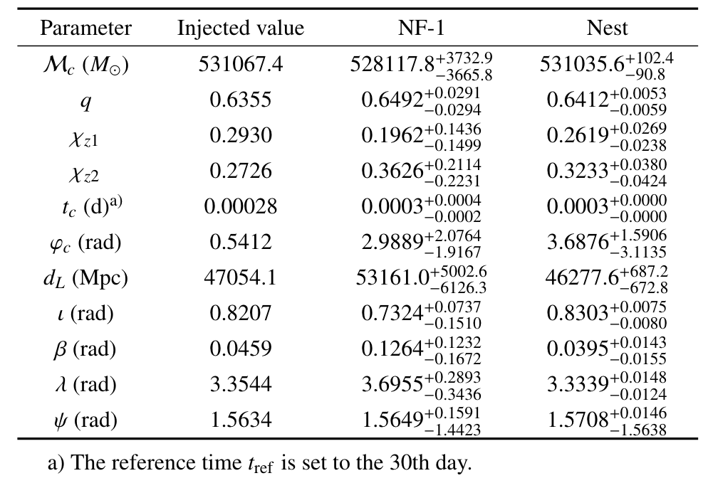
M. Du, B. Liang, HW, P. Xu, Z. Luo, Y. Wu. SCPMA 67, 230412 (2024).
Content

- WaveFormer: Transformer-Based Denoising Method for Gravitational-Wave Data
- Advancing Space-Based Gravitational Wave Astronomy: Rapid Detection and Parameter Estimation Using Normalizing Flows.
-
Overview and Outlook
- Summary & Review
- Ongoing & Future Plan
Summary & Review
- During my postdoc at ICTP-AP, I focused on GW astronomy and integrating AI for analyzing GW signal processing.
- My research emphasized advancing detection technologies from from ground-based to space-based GW detection, setting the stage for future technologies.
在站期间的论文发表情况
- 王赫, 杜明辉, 徐鹏, 周宇峰. 空间引力波探测科学数据处理的挑战与人工智能技术的应用. 中国科学: 物理学 力学 天文学 (2024年6月), 54: doi: 10.1360/SSPMA-2024-0087
- He Wang, Yue Zhou, Zhoujian Cao, Zongkuan Guo, and Zhixiang Ren. “WaveFormer: Transformer-Based Denoising Method for Gravitational-Wave Data.” Machine Learning: Science and Technology 5, no. 1 (March 2024): 015046.
- Wen-Hong Ruan*, He Wang*, Chang Liu, Zong-Kuan Guo. "Rapid search for massive black hole binary coalescences using deep learning." Physics Letters B (2023): 137904. arXiv:2111.14546 [astro-ph.IM] (共同第一作者)
- Minghui Du, Bo Liang, He Wang*, Peng Xu, Ziren Luo, and Yueliang Wu*. “Advancing Space-Based Gravitational Wave Astronomy: Rapid Detection and Parameter Estimation Using Normalizing Flows.” SCIENCE CHINA Physics, Mechanics & Astronomy 67, no. 3 (August 10, 2023): 230412-.
(共同通讯作者) - Marlin B. Schäfer, Ondřej Zelenka, Alexander H. Nitz, He Wang, Shichao Wu, Zong-Kuan Guo, Zhoujian Cao, Zhixiang Ren, Paraskevi Nousi, Nikolaos Stergioulas, Panagiotis Iosif, Alexandra E. Koloniari, Anastasios Tefas, Nikolaos Passalis, Francesco Salemi, Gabriele Vedovato, Sergey Klimenko, Tanmaya Mishra, Bernd Brügmann, Elena Cuoco, E. A. Huerta, Chris Messenger, Frank Ohme. “First Machine Learning Gravitational-Wave Search Mock Data Challenge.” Phys.Rev. D107 (2023) 2, 023021. (算法团队第一作者)
- Wenhong Ruan, He Wang, Chang Liu, and Zongkuan Guo. “Parameter Inference for Coalescing Massive Black Hole Binaries Using Deep Learning.” Universe 9, no. 9 (September 6, 2023): 407.
- Tianyu Zhao, Ruoxi Lyu, Zhixiang Ren, He Wang, Zhoujian Cao. "Space-based gravitational wave signal detection and extraction with deep neural network.” Communications Physics, 2023, 6(1): 212.
- Yuxiang Xu, Minghui Du, Peng Xu, Bo Liang, and He Wang. “Gravitational Wave Signal Extraction Against Non-Stationary Instrumental Noises with Deep Neural Network.” arXiv:2402.13091 [gr-qc]
- Qianyun Yun, Wen-Biao Han, Yi-Yang Guo, He Wang, and Minghui Du. “The Detection, Extraction and Parameter Estimation of Extreme-Mass- Ratio Inspirals with Deep Learning.” arXiv, November 30, 2023. arXiv:2311.18640 [gr-qc]
- Qianyun Yun, Wen-Biao Han, Yi-Yang Guo, He Wang, and Minghui Du. “Detecting Extreme-Mass-Ratio Inspirals for Space-Borne Detectors with Deep Learning.” arXiv, September 12, 2023. arXiv:2309.06694 [gr-qc]
- Cunliang Ma, Wei Wang, He Wang, and Zhoujian Cao. “Artificial Intelligence Model for Gravitational Wave Search Based on the Waveform Envelope.” Phys.Rev. D107(2023) 6, 063029.
- Bo-Rui Wang, Jin Li, and He Wang. “Probing the Gravitational Wave Background from Cosmic Strings with the Alternative LISA-TAIJI Network.” The European Physical Journal C 83, no. 11 (November 7, 2023): 1010.
在站期间的基金申请情况
-
《引力波探测中关于智能降噪和信号搜寻的研究》(已结题)
-
2023-01 ~ 2023-12
-
国自然基金委 | 理论物理专款研究项目 | 18万元 | 负责人
-
在该专款研究项目中负责了从引力波数据的生成,到数据集的制备,到算法模型的搭建,最后到引力波科学数据分析,涉及完整的数据处理流水线的设计和开发。
-
-
《基于引力波探测开源数据的共享数据门户》
-
2023-06 ~ 2025-05
-
国家天文科学数据中心 | 青年数据科学家项目 | 10万元 | 负责人
-
在该专款研究项目中负责构建一个引力波探测开源数据平台,通过采集、整合和管理引力波观测数据和科学分析结果,为科研人员和相关单位提供便捷的数据访问和应用服务,未来有望成为我国空间引力波探测计划的科学基础设施的一部分。
-
在站期间的其他学术活动及任职情况
- 2023.11-2024.1《引力波数据探索:编程与分析实战训练营》太极实验室线上培训
- 2024 年国科大引力波科创计划的本科生指导教师
- 2022-2023年度国家天文科学数据中心青年数据科学家
- 在OpenReview.net上对NeurIPS、ICML、ACL等多个AI顶会和AI4Science Workshop审稿,并受邀担任PLB, MLST等知名期刊的审稿人;《天文技术与仪器(英文)》(Astronomical Techniques and Instruments,ATI)青年编委。
Ongoing & Future Plan
Earth-based GW detection
- A Python Toolbox for Gravitational Wave Astronomy: GWToolkit
- This toolbox is powered by Ray/JAX and supports both CPU and GPU. It is designed specifically for machine learning applications.
- Can AI identify new GW events from LIGO data?
- Could this be a GW signal beyond General Relativity (GR)?
- How can we address the issue of strong or unacceptable biases that occur when outputs from AI models are used jointly or in combination to measure properties of a population, sub-population, or ensemble?
(also addressed by 2405.18095)
Text
Space-based GW detection
- “Global fit” challenge
- How can we achieve and accelerate the Bayesian inference through algorithmic innovations?
- Flow-based proposal?
- Transdimensional Nested Sampling?
- How can we leverage powerful LLM-based methods to accomplish this?
- How can we achieve and accelerate the Bayesian inference through algorithmic innovations?
Text

中科院计算机信息中心“东方”超级计算系统 (全国产CPU/GPU)
for _ in range(num_of_audiences):
    print('Thank you for your attention! 🙏')
Ongoing and Future Plan
Earth-based GW detection
- A Python Toolbox for Gravitational Wave Astronomy: GWToolkit
- This toolbox is powered by Ray/JAX and supports both CPU and GPU. It is designed specifically for machine learning applications.
- Can AI identify new GW events from LIGO data?
- Could this be a GW signal beyond General Relativity (GR)?
- How can we address the issue of strong or unacceptable biases that occur when outputs from AI models are used jointly or in combination to measure properties of a population, sub-population, or ensemble?
(also addressed by 2405.18095)
Text
Space-based GW detection
- “Global fit” challenge
- How can we achieve and accelerate the Bayesian inference through algorithmic innovations?
- Flow-based proposal?
- Transdimensional Nested Sampling?
- How can we leverage powerful LLM-based methods to accomplish this?
- How can we achieve and accelerate the Bayesian inference through algorithmic innovations?
Text
Ongoing and Future Plan
| Pipeline | Targets | Programing Language (sampling method) | Comments |
|---|---|---|---|
|
GLASS (Littenberg&Cornish 2023) |
Noise, UCB, VGB, MBHB |
C / Python (TPMCMC / RJMCMC) | noise_mcmc+gb_mcmc+vb_mcmc+global_fit |
| Eryn | UCB | Python (TPMCMC / RJMCMC) | Mini code for UCB case |
| PyCBC-INFERENCE | MBHB | Python (?) | Unavailable |
| Bilby in Space / tBilby | MBHB / ? | ? / Python? (RJMCMC) | Unavailable |
| Strub et al. | UCB | ? (GP) | Unavailable / GPU-based |
| Zhang et al. (LZU) | UCB | ? (PSO) | MLP |
| Balrog | MBHB | ? |
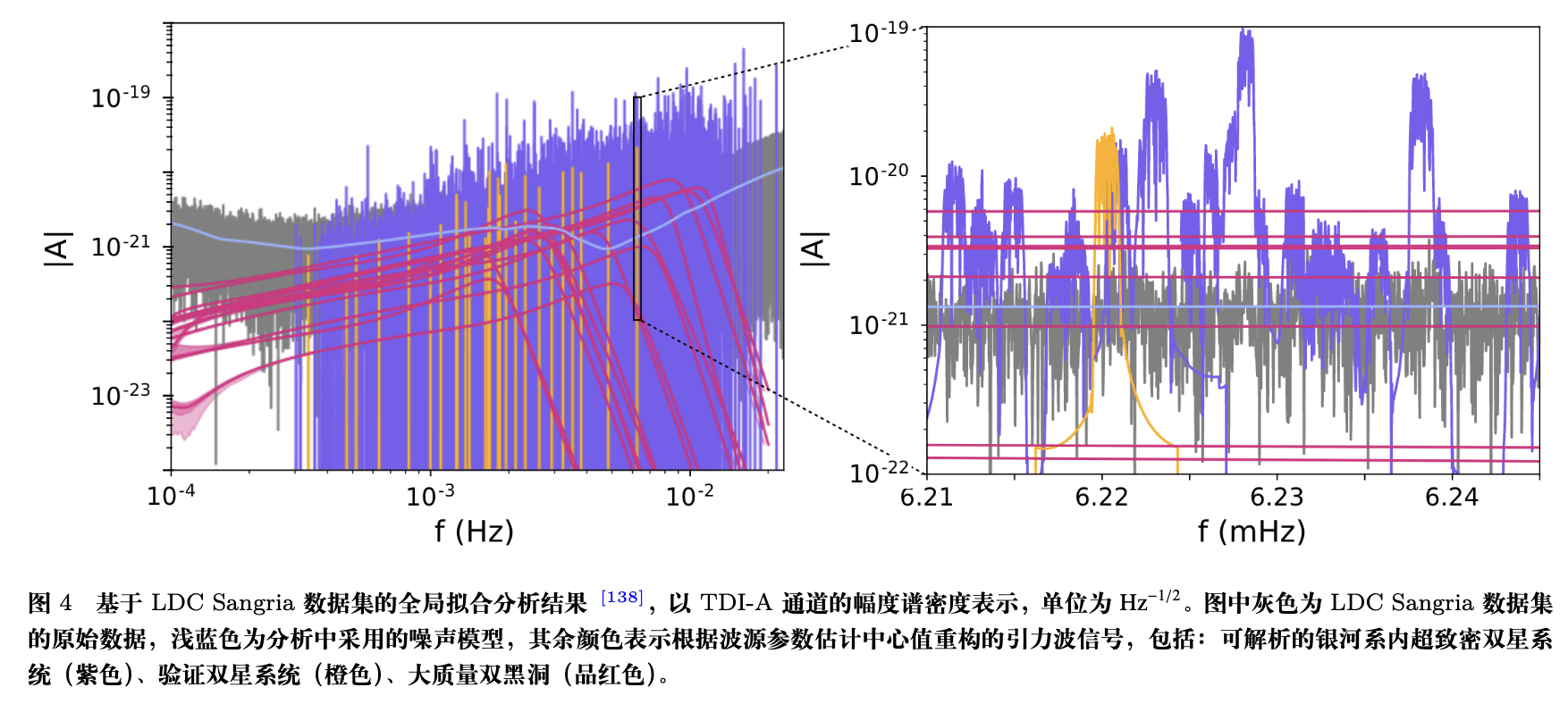
(Sec.8.6 Red Book)
Global Fit
- The idea of the global fit method is to comprehensively model all astrophysical and instrumental features present in the space-borne gravitational wave data.
- This approach not only focuses on the signal from a single source, but attempts to capture the combined effects of all sources in the data, conducting a comprehensive analysis of the entire dataset to identify and model all potential signal and noise sources.
Technical challenges:
- High dimensional
- Highly correlated
- Multimodality
- Trans-dimensional
Text
M. Du, B. Liang, HW, P. Xu, Z. Luo, Y. Wu. SCPMA 67, 230412 (2024).
Ongoing and Future Projects
Neural density estimation
- Density fit for posterior distributions
- use the old posterior to form a proposal for the extended data.
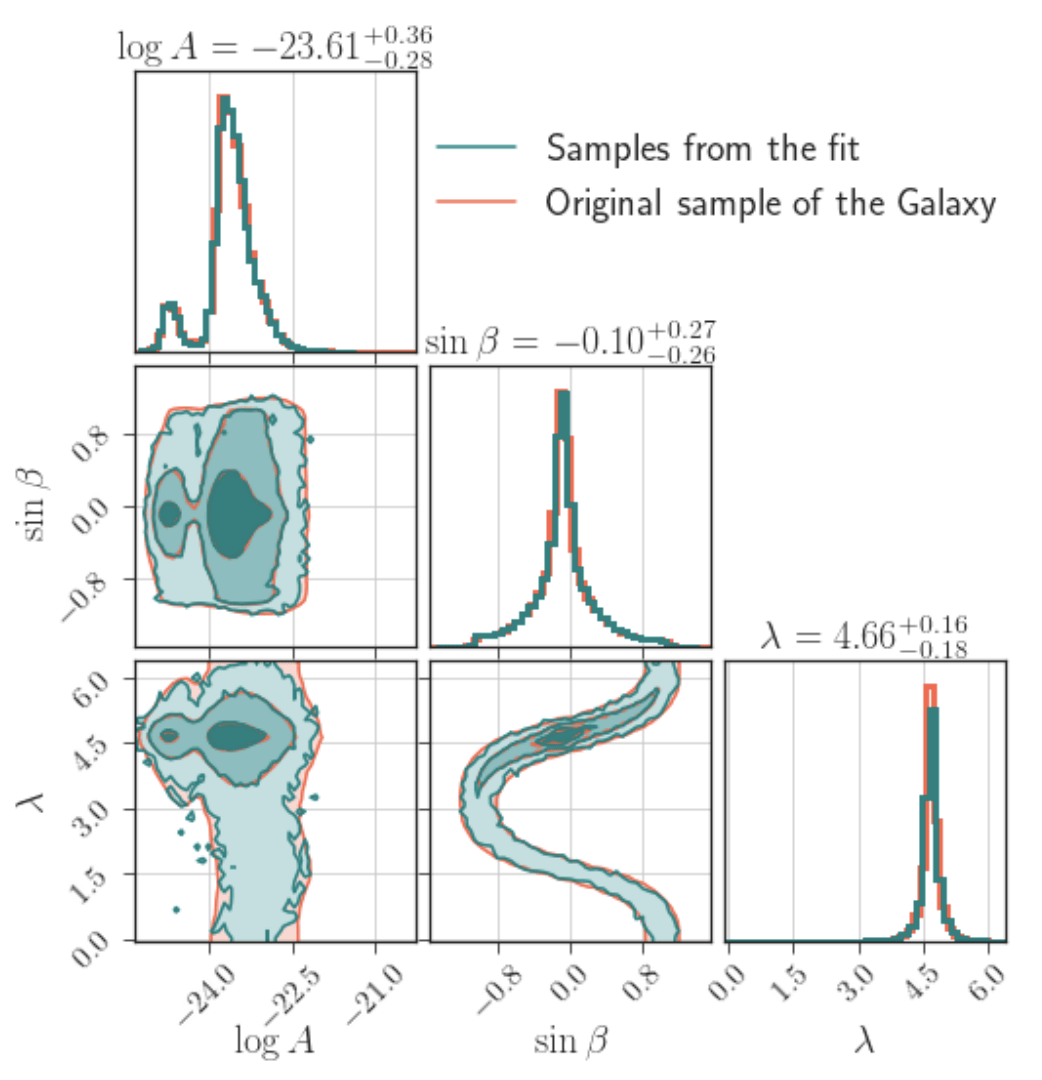
- Density fit for the Galaxy
- fitt a Galaxy model for joint distribution for \((A, \beta, \lambda)\).
- ...
Text
Ref:
- Ashton, G, and C Talbot. MNRAS 507, no. 2 (2021): 2037–51.
- Korsakova, N, et al. (2402.13701)
- Wouters, T, et al. (2404.11397)
Ongoing and Future Projects
Neural density estimation
- Density fit for posterior distributions
- use the old posterior to form a proposal for the extended data.
- Density fit for the Galaxy
- fitt a Galaxy model for joint distribution for \((A, \beta, \lambda)\).
- ...
Text
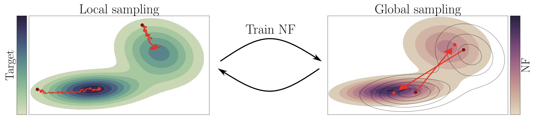
nflow
(Based on 1912.02762)
The ABC of Normalizing Flow
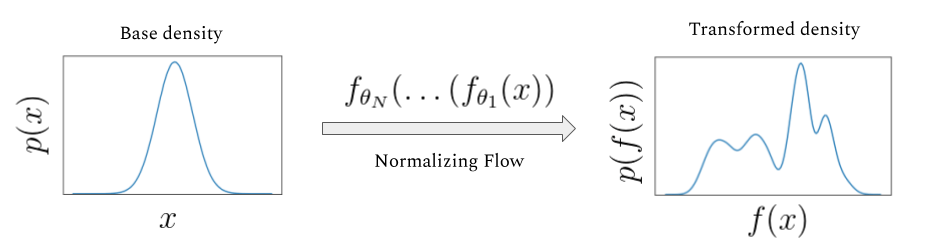
The main idea of flow-based modeling is to express \(\mathbf{y}\in\mathbb{R}^D\) as a transformation \(T\) of a real vector \(\mathbf{z}\in\mathbb{R}^D\) sampled from \(p_{\mathrm{z}}(\mathbf{z})\):
Note: The invertible and differentiable transformation \(T\) and the base distribution \(p_{\mathrm{z}}(\mathbf{z})\) can have parameters \(\{\boldsymbol{\phi}, \boldsymbol{\psi}\}\) of their own, i.e. \( T_{\phi} \) and \(p_{\mathrm{z},\boldsymbol{\psi}}(\mathbf{z})\).
Change of Variables:
Equivalently,
The Jacobia \(J_{T}(\mathbf{u})\) is the \(D \times D\) matrix of all partial derivatives of \(T\) given by:
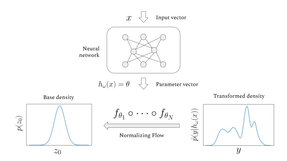
base density
target density
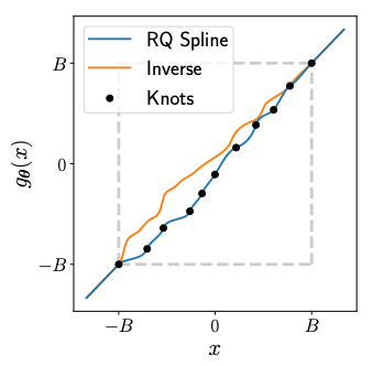
Rational Quadratic Neural Spline Flows (RQ-NSF)
(Based on 1912.02762)
- Data: target data \(\mathbf{y}\in\mathbb{R}^{11}\) (with condition data \(\mathbf{x}\)).
- Task:
- Fitting a flow-based model \(p_{\mathrm{y}}(\mathbf{y} ; \boldsymbol{\theta})\) to a target distribution \(p_{\mathrm{y}}^{*}(\mathbf{y})\)
- by minimizing KL divergence with respect to the model’s parameters \(\boldsymbol{\theta}=\{\boldsymbol{\phi}, \boldsymbol{\psi}\}\),
- where \(\boldsymbol{\phi}\) are the parameters of \(T\) and \(\boldsymbol{\psi}\) are the parameters of \(p_{\mathrm{z}}(\mathbf{z})=\mathcal{N}(0,\mathbb{I})\).
- Loss function:
- Assuming we have a set of samples \(\left\{\mathbf{y}_{n}\right\}_{n=1}^{N}\sim p_{\mathrm{y}}^{*}(\mathbf{y})\),
Minimizing the above Monte Carlo approximation of the KL divergence is equivalent to fitting the flow-based model to the samples \(\left\{\mathbf{y}_{n}\right\}_{n=1}^{N}\) by maximum likelihood estimation.

nflow
nflow
Train
Test
The ABC of Normalizing Flow
Parameter estimation · Scientific discovery
Credit: LIGO Magazine.
-
Traditional parameter estimation (PE) techniques rely on Bayesian analysis methods (posteriors + evidence)
- Computing the full 15-dimensional posterior distribution estimate is very time-consuming:
- Calculating likelihood function
- Template generation time-consuming
- Machine learning algorithms are expected to speed up!
Bayesian statistics
Data quality improvement
Credit: Marco Cavaglià
LIGO-Virgo data processing
GW searches
Astrophsical interpretation of GW sources
Background
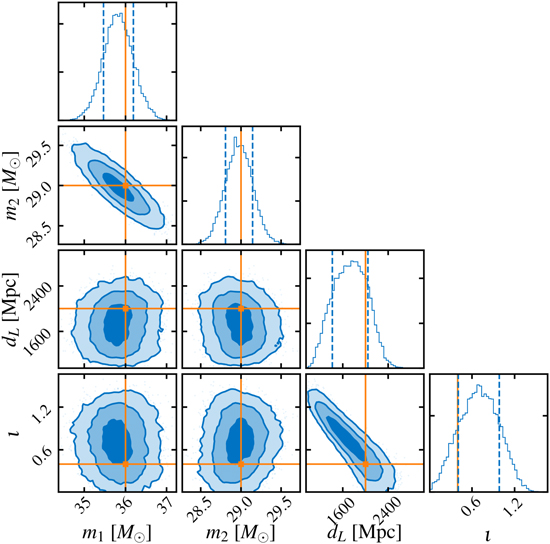
- A complete 15-dimensional posterior probability distribution, taking about 1 s (<< \(10^4\) s).
- Prior Sampling: 50,000 Posterior samples in approximately 8 Seconds.
- Capable of calculating evidence
- Processing time: (using 64 CPU cores)
- less than 1 hour with IMRPhenomXPHM,
- approximately 10 hours with SEOBNRv4PHM
PRL 127, 24 (2021) 241103.
PRL 130, 17 (2023) 171403.
Nature Physics 18, 1 (2022) 112–17
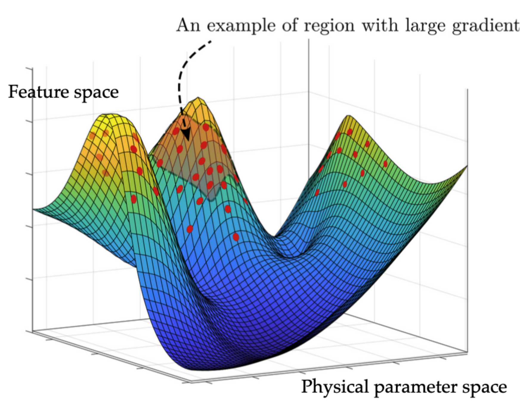
HW, et al. Big Data Mining and Analytics 5, 1 (2021) 53–63.
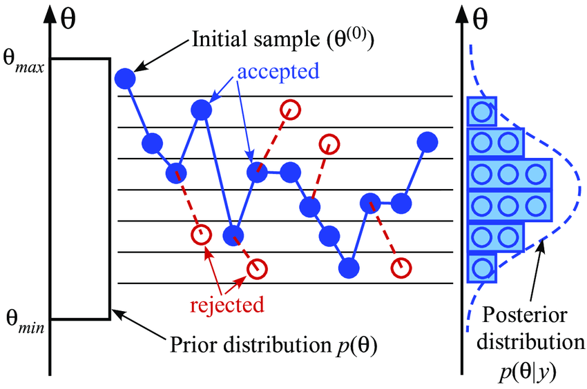
A diagram of prior sampling between feature space and physical parameter space