Particle Swarm Optimization (PSO)
This slide: https://slides.com/iphysresearch/pso
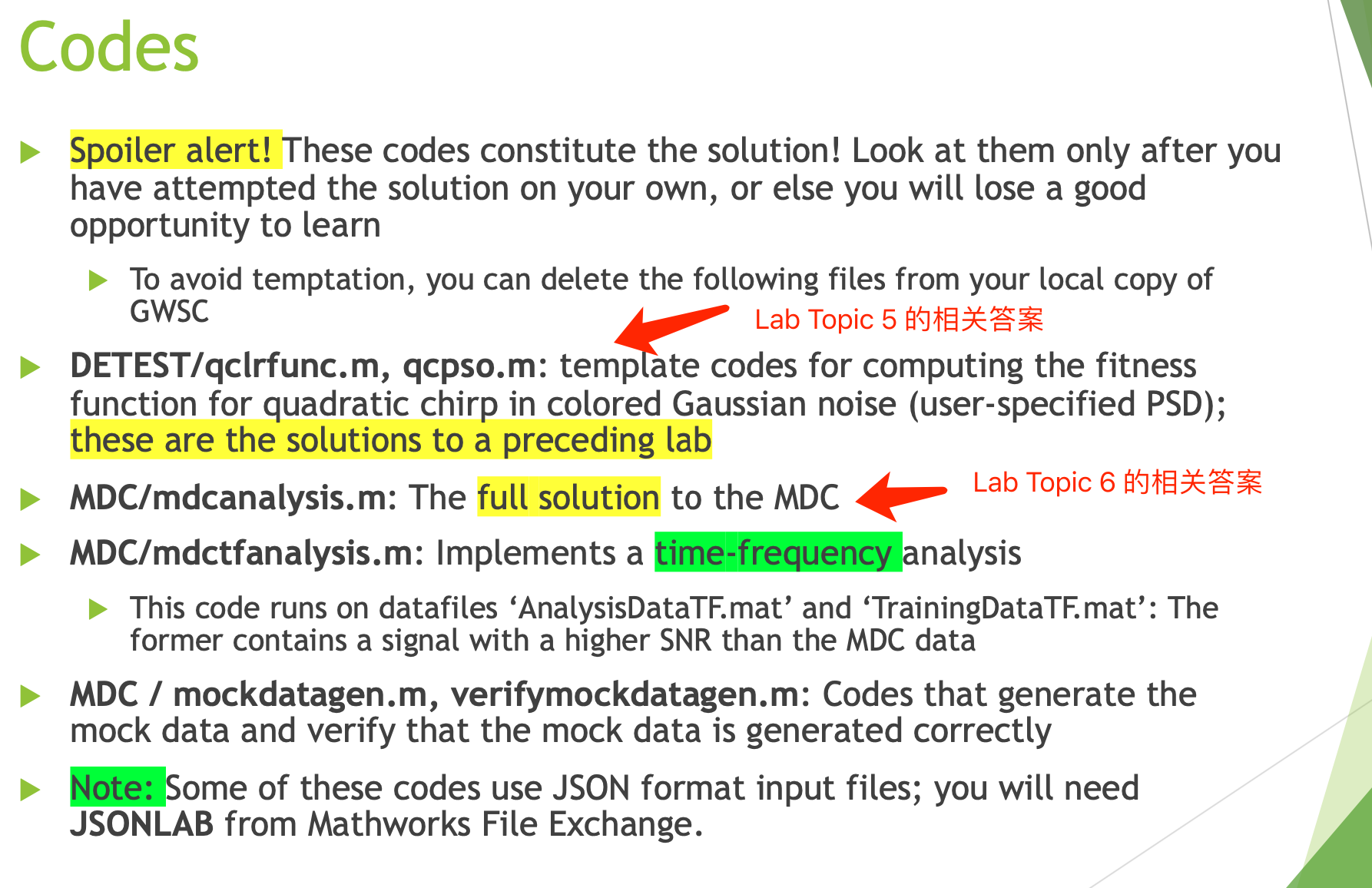
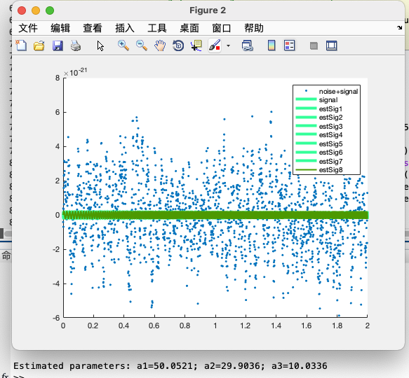
Particle Swarm Optimization (PSO)
This slide: https://slides.com/iphysresearch/pso
function innProd = innerprodpsd(xVec,yVec,sampFreq,psdVals)
%P = INNERPRODPSD(X,Y,Fs,Sn)
%Calculates the inner product of vectors X and Y for the case of Gaussian
%stationary noise having a specified power spectral density. Sn is a vector
%containing PSD values at the positive frequencies in the DFT of X
%and Y. The sampling frequency of X and Y is Fs.

%Soumya D. Mohanty, Mar 2019

nSamples = length(xVec);
if length(yVec) ~= nSamples
    error('Vectors must be of the same length');
end
kNyq = floor(nSamples/2)+1;
if length(psdVals) ~= kNyq
    error('PSD values must be specified at positive DFT frequencies');
end

fftX = fft(xVec);
fftY = fft(yVec);
%We take care of even or odd number of samples when replicating PSD values
%for negative frequencies
negFStrt = 1-mod(nSamples,2);
psdVec4Norm = [psdVals,psdVals((kNyq-negFStrt):-1:2)];

dataLen = sampFreq*nSamples;

innProd = (1/dataLen)*(fftX./psdVec4Norm)*fftY';
innProd = real(innProd);
def innerprodpsd(xVec,yVec,sampFreq,psdVals):
"""
P = INNERPRODPSD(X,Y,Fs,Sn)
Calculates the inner product of vectors X and Y for the case of Gaussian
stationary noise having a specified power spectral density. Sn is a vector
containing PSD values at the positive frequencies in the DFT of X
and Y. The sampling frequency of X and Y is Fs.
Soumya D. Mohanty, Mar 2019
He Wang
Mar 2021: Adapted for python
"""
nSamples = len(xVec)
assert len(yVec) == nSamples, 'Vectors must be of the same length'
kNyq = np.floor(nSamples/2)+1
assert len(psdVals) == kNyq, 'PSD values must be specified at positive DFT frequencies'
# Why 'scipy.fftpack.fft'?
# See: https://iphysresearch.github.io/blog/post/signal_processing/fft/#efficiency-of-the-algorithms
fftX = fft(xVec)
fftY = fft(yVec)
#We take care of even or odd number of samples when replicating PSD values
#for negative frequencies
negFStrt = 1 - np.mod(nSamples, 2)
psdVec4Norm = np.concatenate((psdVals, psdVals[(kNyq.astype('int')-negFStrt)-1:0:-1]))
dataLen = sampFreq * nSamples
innProd = np.sum((1/dataLen) * (fftX / psdVec4Norm)*fftY.conj())
innProd = np.real(innProd)
return innProdMATLAB
Python
Particle Swarm Optimization (PSO)

This slide: https://slides.com/iphysresearch/pso
# Python
from scipy.signal import firwin2, firwin

f1 = firwin(30+1, (30/256), pass_zero='lowpass',)
f2 = firwin(30+1, [(30/256), 50/256], pass_zero='bandpass',)
f2 = firwin(30+1, (30/256), pass_zero='highpass',)

ff = firwin2(150+1, [0.0, 0.5, 1.0], [1.0, 1.0, 0.0])
# MATLAB
f1 = fir1( 30, 30/2/(256/2), 'low' )
f2 = fir1( 30, [(30)/2/(256/2),(50)/2/(256/2)], 'bandpass' )
f3 = fir1( 30, 30/2/(256/2), 'high' )
ff = fir2(150,[0.0, 0.5, 1.0], [1.0, 1.0, 0.0])partCoord
partVel
partPbest
partLocalBest
-1
1
0
partFitPbest
partFitCurr
partFitLbest
partInertia
partFlagFitEval
partFitEvals
gbestVal
gbestLoc
bestFitness
-
partCoord: Particle location
-
partVel: Particle velocity
-
partPbest: Particle pbest
-
partFitPbest: Fitness value at pbest
-
partFitCurr: Fitness value at current iteration
-
partFitLbest: Fitness value at local best location
-
partInertia: Inertia weight
-
partLocalBest: Particles local best location
-
partFlagFitEval: Flag whether fitness should be computed or not
-
partFitEvals: Number of fitness evaluations
-
gbestVal: Best value found by the swarm over its history
-
gbestLoc: Location of the best value found by the swarm over its history
-
bestFitness: Best value found by the swarm at the current iteration
Initialization
0
1
popsize = 40
Number of PSO particles
pop
Step.0: Specify information about each particle stored as a row of a matrix ('pop').

Fitness
Location
partCoord
partVel
partPbest
partLocalBest
k th
-1
1
0
partFitPbest
partFitCurr
partFitLbest
partInertia
partFlagFitEval
partFitEvals
gbestVal
gbestLoc
bestFitness
Start PSO iterations
fitfuncHandle
(glrtqcsig4pso)
Step.1: for each particle, update partFitCurr / partFitEvals / partFitPbest / partPbest.
Output from your fitness function
Escape from special boundary condition
partFitCurr
for each particle
0
1
partPbest
partCoord
popsize = 40
Number of PSO particles
partFitCurr
partFitPbest
partCoord
partFitLbest
pop
if partFlagFitEval
partFitEvals += 1
partFitEvals += 0
- For each particle, record the best location and fitness value over its history.
(记录个人历史最好成绩)

Fitness
Location
partCoord
partVel
partPbest
partLocalBest
k' th
0
1
-1
1
0
partFitPbest
partFitCurr
partFitLbest
partInertia
partFlagFitEval
partFitEvals
gbestVal
gbestLoc
bestFitness
fitfuncHandle
(glrtqcsig4pso)
Step.2: for all particles, update gbestLoc / gbestVal.
Output from your fitness function
find the global minimum
gbestVal
gbestLoc
+=1
partCoord
popsize = 40
Number of PSO particles
partFitCurr
partCoord
pop
Start PSO iterations
- For all particles, record the best location and fitness value over their history.
(记录全局历史最好成绩)

Fitness
Location
partCoord
partVel
partPbest
partLocalBest
k th
popsize = 40
Number of PSO particles
0
1
-1
1
0
partFitLbest
partInertia
partFlagFitEval
partFitEvals
gbestVal
gbestLoc
bestFitness
fitfuncHandle
(glrtqcsig4pso)
Step.3: for local neighborhood of each particle, update partFitLbest / partLocalBest.
Output from your fitness function
find the local minimum
partFitPbest
partFitCurr
partLocalBest
partCoord
nbrhdSz \(\le\) 3
Number of particles in a ring topology neighborhood.
partFitLbest
partFitCurr
partCoord
pop
Eg:
For particle 1, its local neighborhood is: [5 1 2]
For particle 2, its local neighborhood is: [1 2 3]
For particle 3, its local neighborhood is: [2 3 4]
For particle 4, its local neighborhood is: [3 4 5]
For particle 5, its local neighborhood is: [4 5 1]
Start PSO iterations
- For each particle, record the best location and fitness value of its local neighborhood.
(记录局部历史最好成绩)

Fitness
Location
pop
partCoord
partVel
partPbest
partLocalBest
k th
popsize = 40
Number of PSO particles
0
1
-1
1
0
partFitLbest
partInertia
partFlagFitEval
partFitEvals
gbestVal
gbestLoc
bestFitness
Step.4: for each particle (update velocity), update partVel / partFitCurr / partFlagFitEval.
partFitPbest
partFitCurr
partInertia \(\times\) partVel + \(c_1\) \(\times\) \(\chi_1\) \(\times\) ( partPbest - partCoord ) + \(c_2\) \(\times\) \(\chi_2\) \(\times\) ( partLocalBest - partCoord )
NEW partVel
partCoord +
NEW partVel
NEW partCoord
Start PSO iterations

- For each particle, record the difference (velocity) in current iteration, update its coordinate.
(记录位置偏移量,更新各自的位置)
Fitness
Location

pop
partCoord
partVel
partPbest
partLocalBest
k th
popsize = 40
Number of PSO particles
0
1
-1
1
0
partFitLbest
partInertia
partFlagFitEval
partFitEvals
gbestVal
gbestLoc
bestFitness
Step.4: for each particle (update velocity), update partVel / partFitCurr / partFlagFitEval.
partFitPbest
partFitCurr
partInertia \(\times\) partVel + \(c_1\) \(\times\) \(\chi_1\) \(\times\) ( partPbest - partCoord ) + \(c_2\) \(\times\) \(\chi_2\) \(\times\) ( partLocalBest - partCoord )
NEW partVel
partCoord +
NEW partVel
NEW partCoord
Start PSO iterations

- For each particle, record the difference (velocity) in current iteration, update its coordinate.
(记录位置偏移量,更新各自的位置)
Fitness
Location
Step.0
Step.1
Step.2
Step.3
Step.4
maxStep = 2000
Number of iterations for termination
nRuns = 8
Number of independent PSO runs
First run of PSO

Fitness
Location
"Particle Swarm Optimization Visually Explained":
https://towardsdatascience.com/particle-swarm-optimization-visually-explained-46289eeb2e14
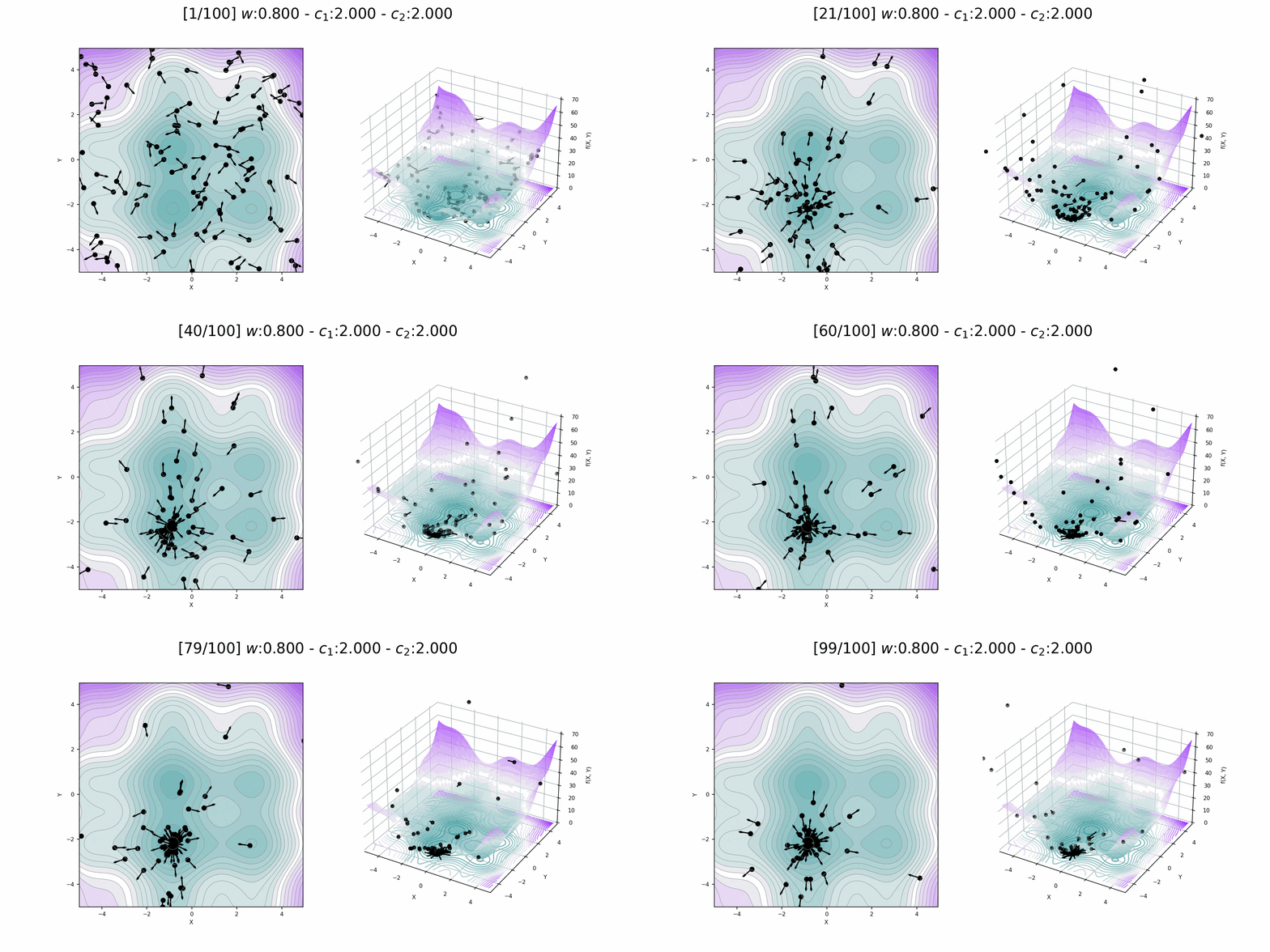

Inertia weight comparison

Fitness
Location
"Particle Swarm Optimization Visually Explained":
https://towardsdatascience.com/particle-swarm-optimization-visually-explained-46289eeb2e14
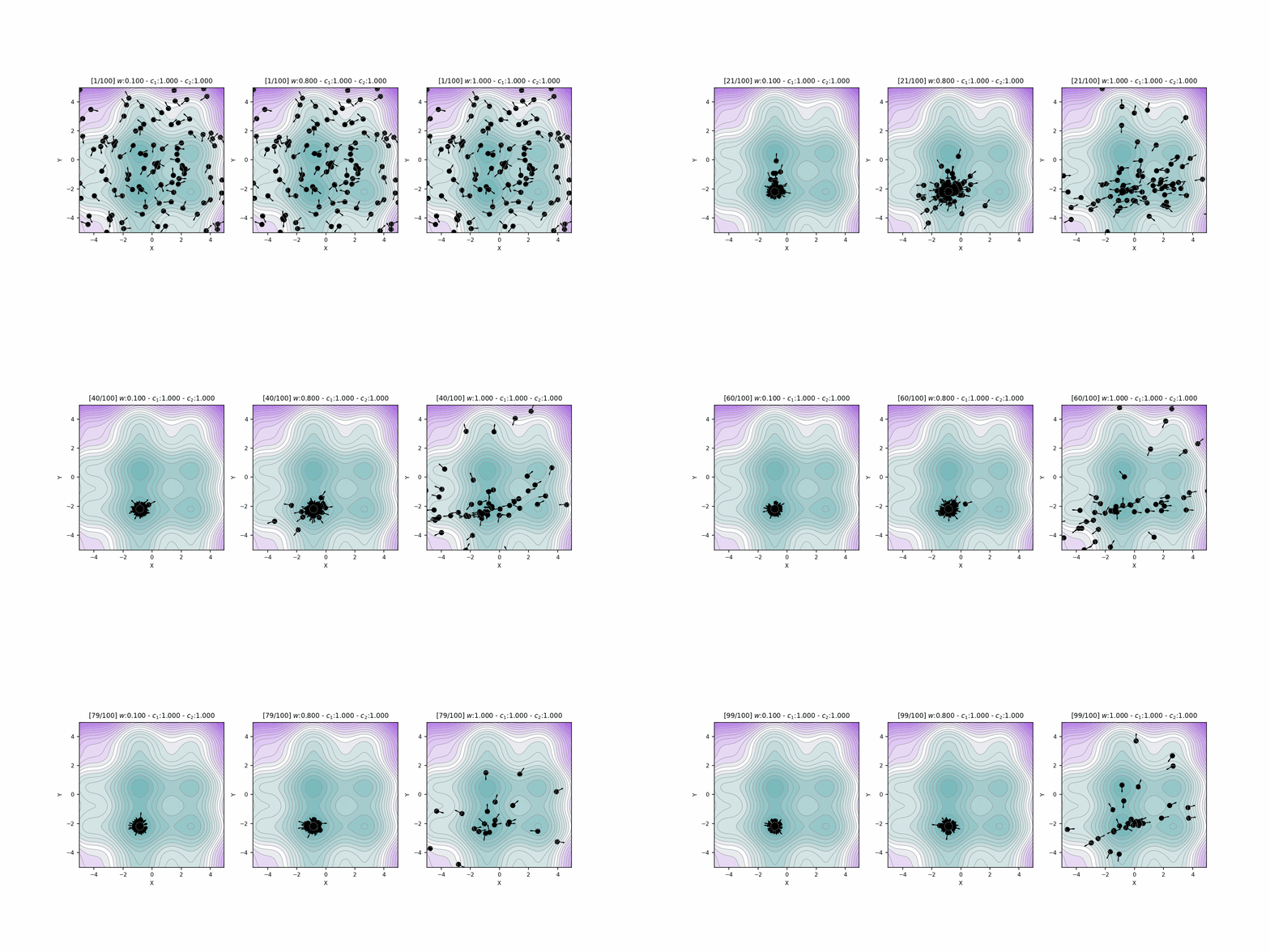

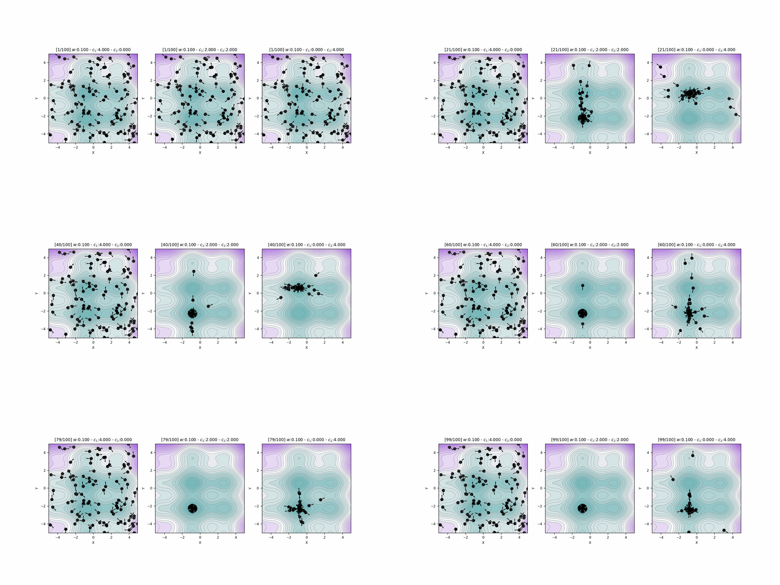
Hyperparameter \(c_1\), \(c_2\) comparison

Fitness
Location
"Particle Swarm Optimization Visually Explained":
https://towardsdatascience.com/particle-swarm-optimization-visually-explained-46289eeb2e14

for _ in range(num_of_audiences):
    print('Thank you for your attention! 🙏')