A Theory of Cluster Patterns in Tensors
2025 James B. Wilson

https://slides.com/jameswilson-3/cluster-patterns-theory/
Tensors as area & volume

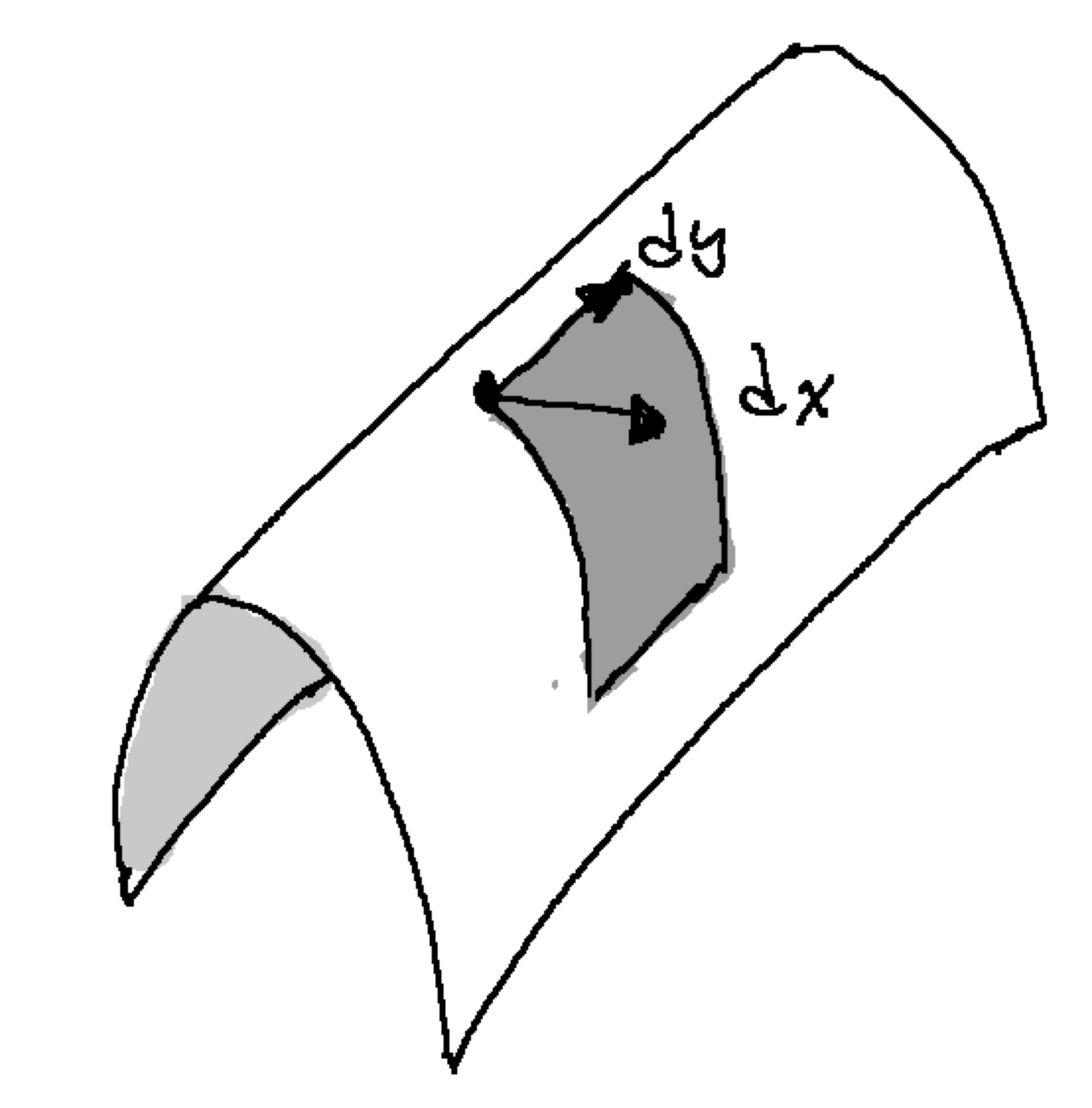
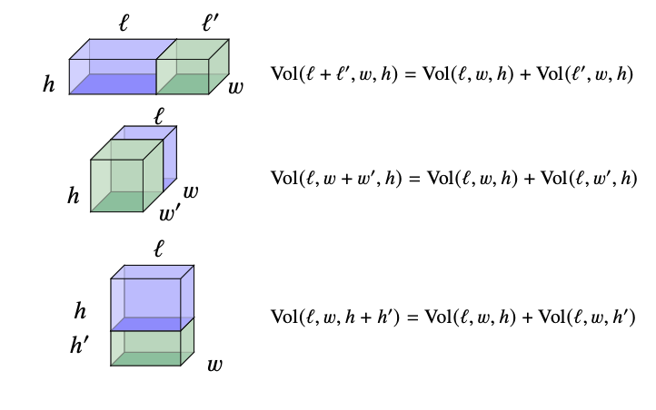
Volume basics
\[Vol(\ell, w,h)= \ell\times w\times h\]
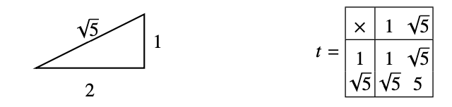
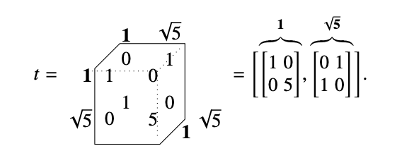
Volume reality
\[Vol(t\mid \ell, w,h)= t\times \ell\times w\times h\] where \(t\) converts miles/meters/gallons/etc.
tensor conversion
Miles
Yards
Feet
Gallons
Area...easy
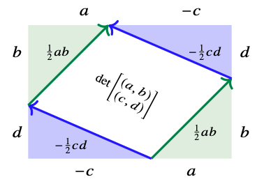
Area...not so easy
\[det\left(\begin{array}{c} (a,b)\\ (c,d)\end{array}\right) = ad-bc\]
\[= \begin{bmatrix} a & b\end{bmatrix}\begin{bmatrix} 0 & 1 \\ -1 & 0 \end{bmatrix}\begin{bmatrix} c\\ d \end{bmatrix}\]
tensor
Tensor's as Multiplication Tables
Notation
\[a*e*\cdots *u\qquad [u,v]\qquad a\otimes e\otimes \cdots \otimes u\] \[[a,e,\ldots, u]\qquad \langle a,e,\ldots, u\rangle\]
Choose a heterogenous product notation
Choose index yoga, mine is "functional", i.e. \(v\in \prod_{a\in A} U_a\)
\[\langle v\rangle =\langle v_1,\ldots, v_{\ell}\rangle= \langle v_a,v_{\bar{a}}\rangle\qquad \{1,\ldots,\ell\}=\{a\}\sqcup\bar{a}\]
When explicit tensor data \(t\)
\[\langle t\mid v\rangle =\langle t \mid v_B,v_C\rangle \qquad A=B\sqcup C\]
\(v\in \prod_{a\in A} V_a\) means \(v:A\to \bigcup_{a\in A} V_a\) with \(v_a\in V_a\).
\(v_B\) is restriction of the function to \(B\subset A\)
\((v_B,v_C)\) is disjoint union of functions \(B\sqcup C\to \bigcup_{e\in B\sqcup C} V_e\)
Technical Requirements
Each space \(V_a\) needs a suite of (multi-)sums
Product commutes with sums ("Distribution/Multi-additive")
\(\displaystyle \int_I v_a(i) d\mu\) could be various sum algorithms "sum(vs[a],method54)"
For \(\{v_a(i)\mid i\in I\}\)
\[\int_I \langle v_a(i),v_{\bar{a}}\rangle\,d\mu = \left\langle \int_I v_a(i)\,d\mu,v_{\bar{a}}\right\rangle\]
Sums are entropic/Fubinian
\[\int_I \int_J f\, d\mu d\nu=\int_J\int_I f \, d\nu d\mu\]
Theory
TL;DR tensors behave like your algebra teacher told you (almost).
Murdoch-Toyoda Bruck
All entropic sums that can solve equations \(a+x=b\) are affine.
Eckmann-Hilton
Entropic sums with 0 are associative & commutative.
Grothendieck
You can add negatives.
Mal'cev, Miyasnikov
You can enrich distributive products with universal scalars.
Davey-Davies
Tensor algebra is ideal determined precisely for affine.
First-Maglione-Wilson
Full classification of algebraic enrichment:
- If 3 or more positions must be Lie
- 2 can be associative or Jordan.
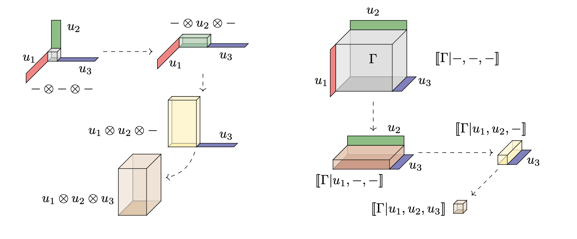
Illustrating Tensor Product/Contraction
(Aka. Inner/Outer products, Co-multiply/Multiply)
Inflate: data of product stored as a bigger array.
Contract: integral of data stored in smaller array.
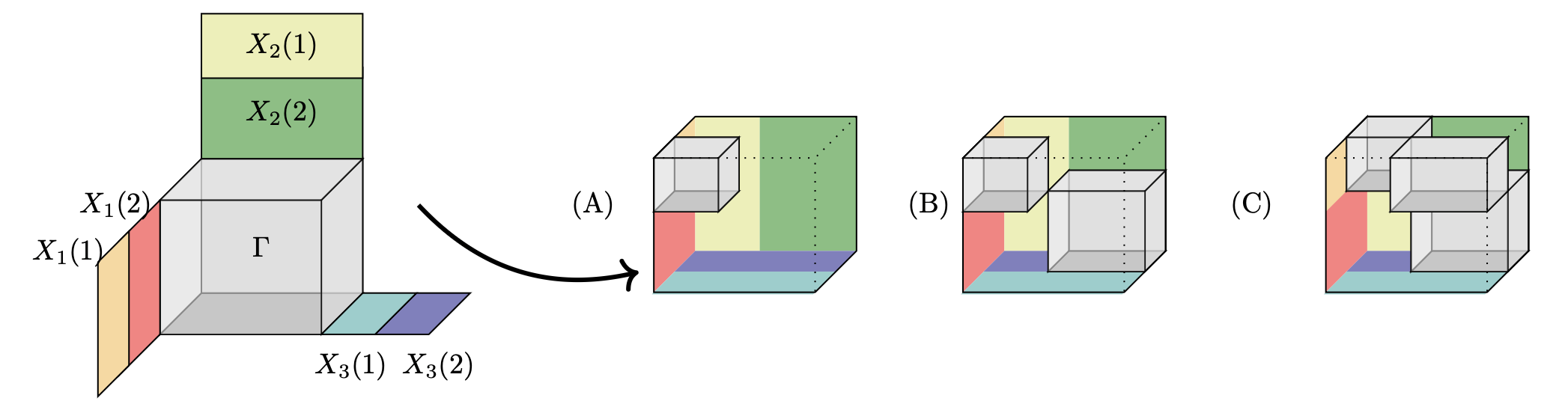
Illustrating manipulating tensors
-
Shaded gray illustrates possibly non-zero
-
A basis of vectors contracted on each side stacks up contractions to reconstitute a new tensor.
New uses? Sales Volume?
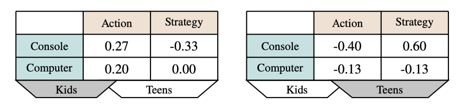
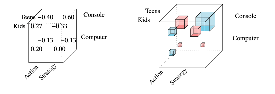
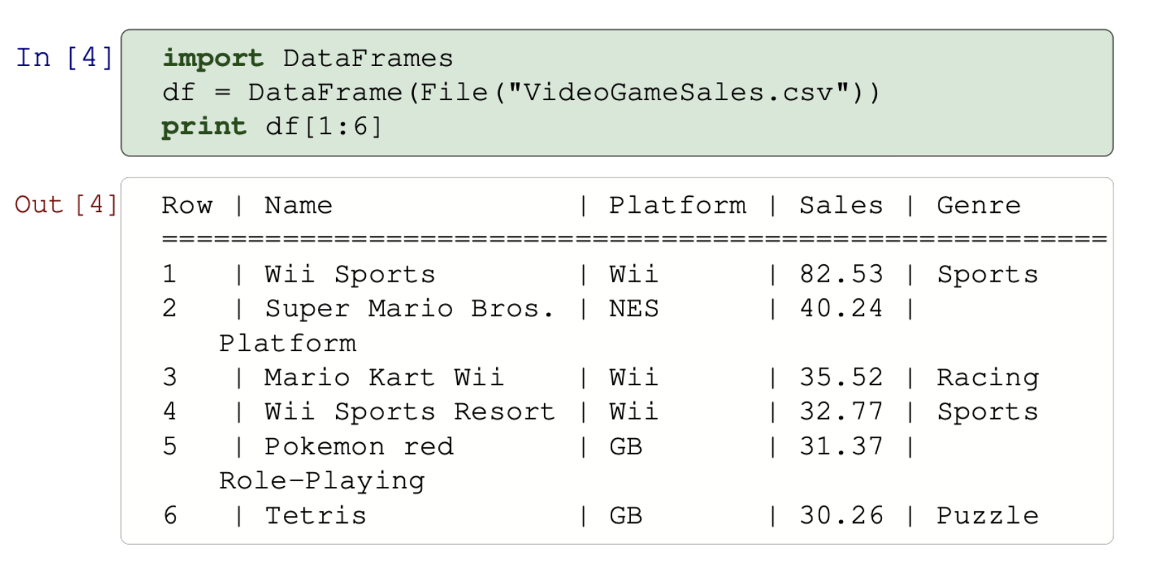
Data science tensors
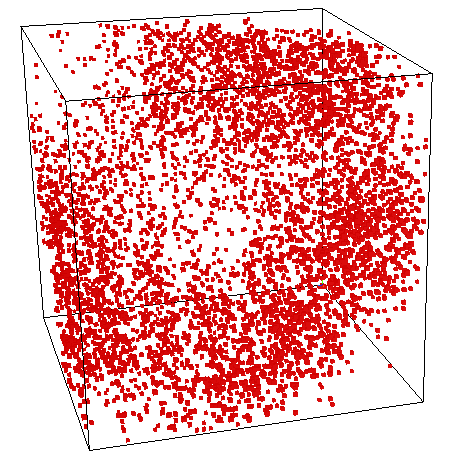
Histogram Visualization
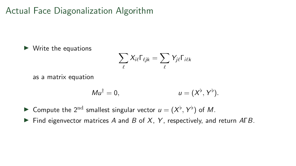
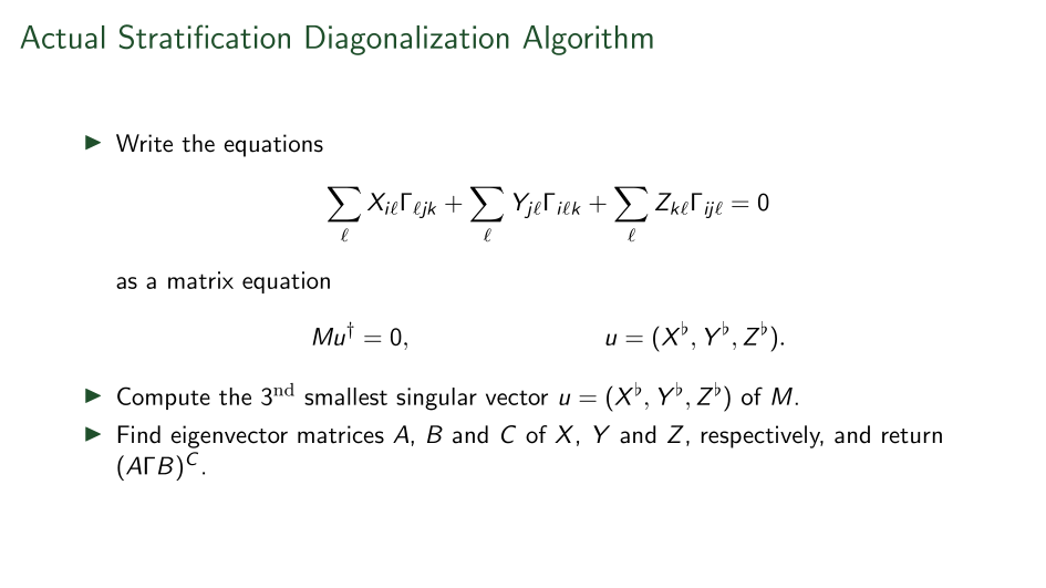
What we have found is computable.
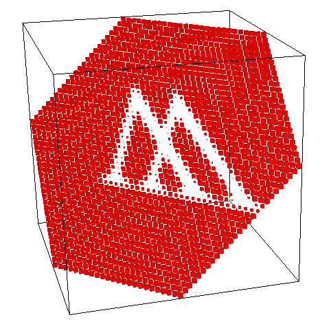
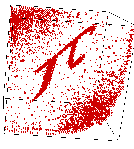
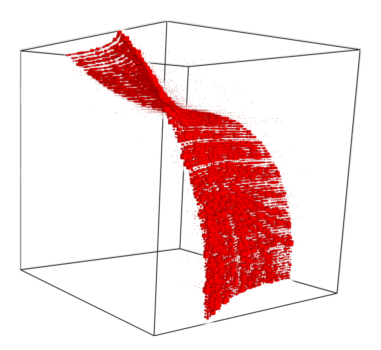
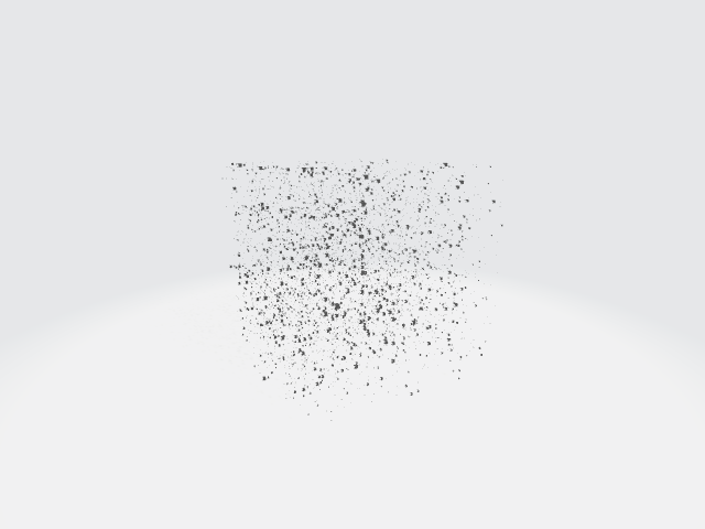
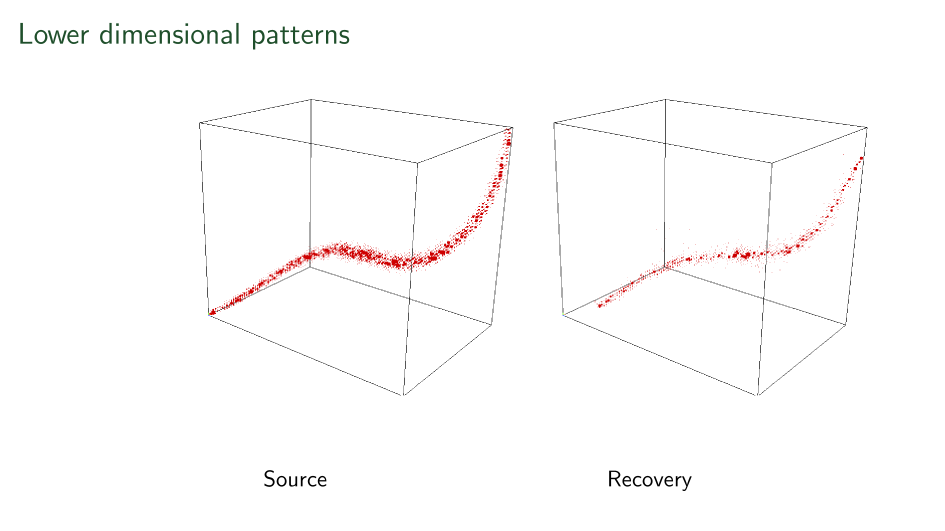
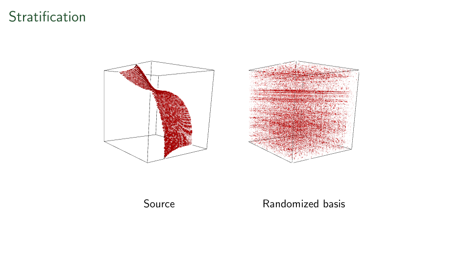
"Random" Basis Change
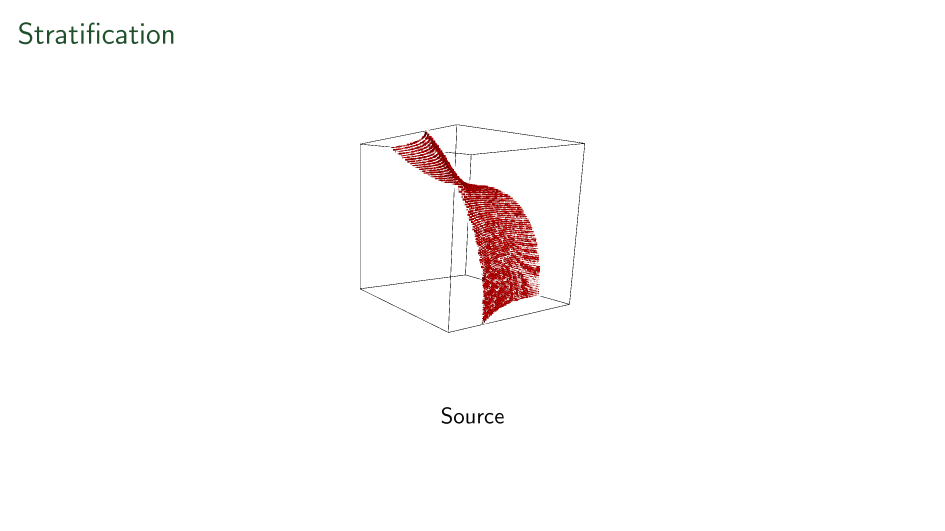
Our blind source separation
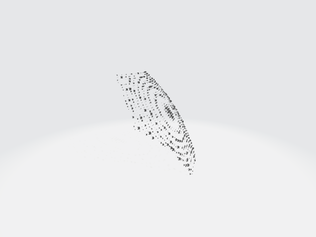
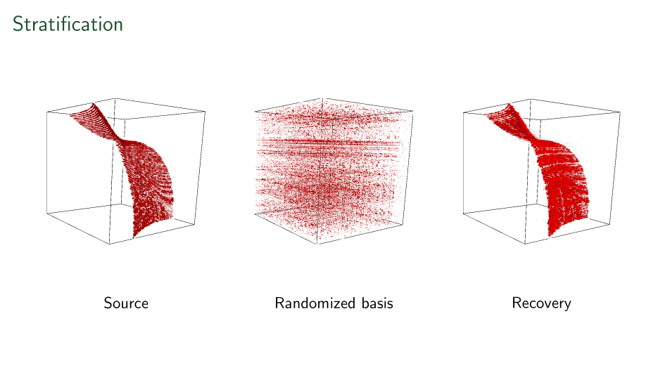
First ever stratification
Shown here is a linear-time recovered unique basis change applied to each side of a tensor to make it's support on a surface.
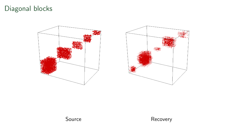
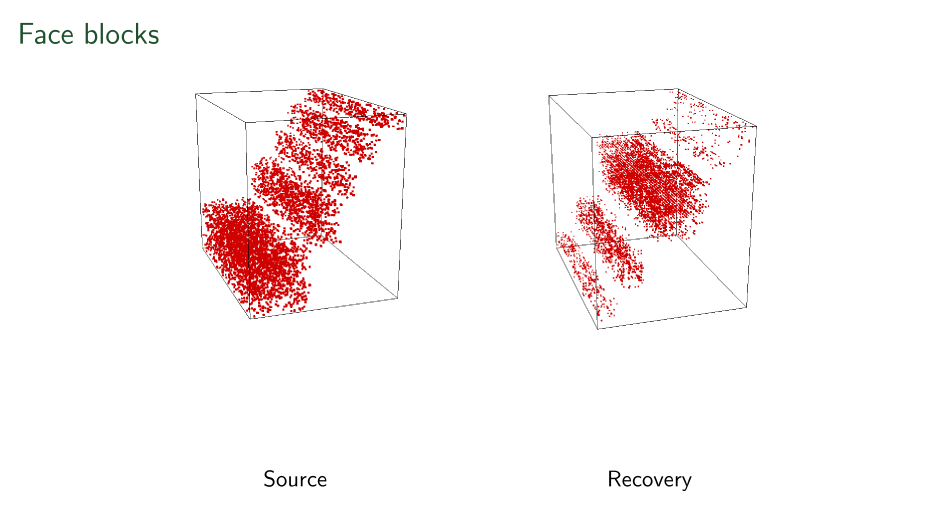
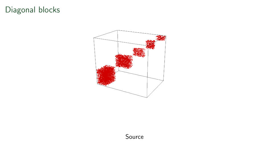
Blocks have been seen before
- Mal'cev folklore credited by numerous Russian papers.
- Miyasnikov in Model Theory Tensors
- Cardoso 1991 Statistical tensors
- Eberly-Geisbrecht 2000 Algebraic tensors
- Acar et. al. 2005 Data science
- W. 2007/8 Central/Direct products of p-groups
-
Maehara and K. Murota, 2010.
- Lathauwer 2008 Small rank cases
- 2024+ Liu-Maglione-W. \(O(d^{1.5\omega+n})\)-time solution (n=valence, d=max dimension, \(\omega\)=matrix mult. exp.).
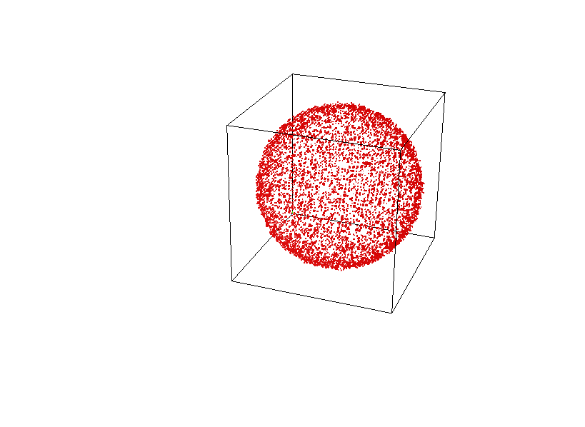
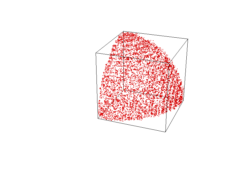
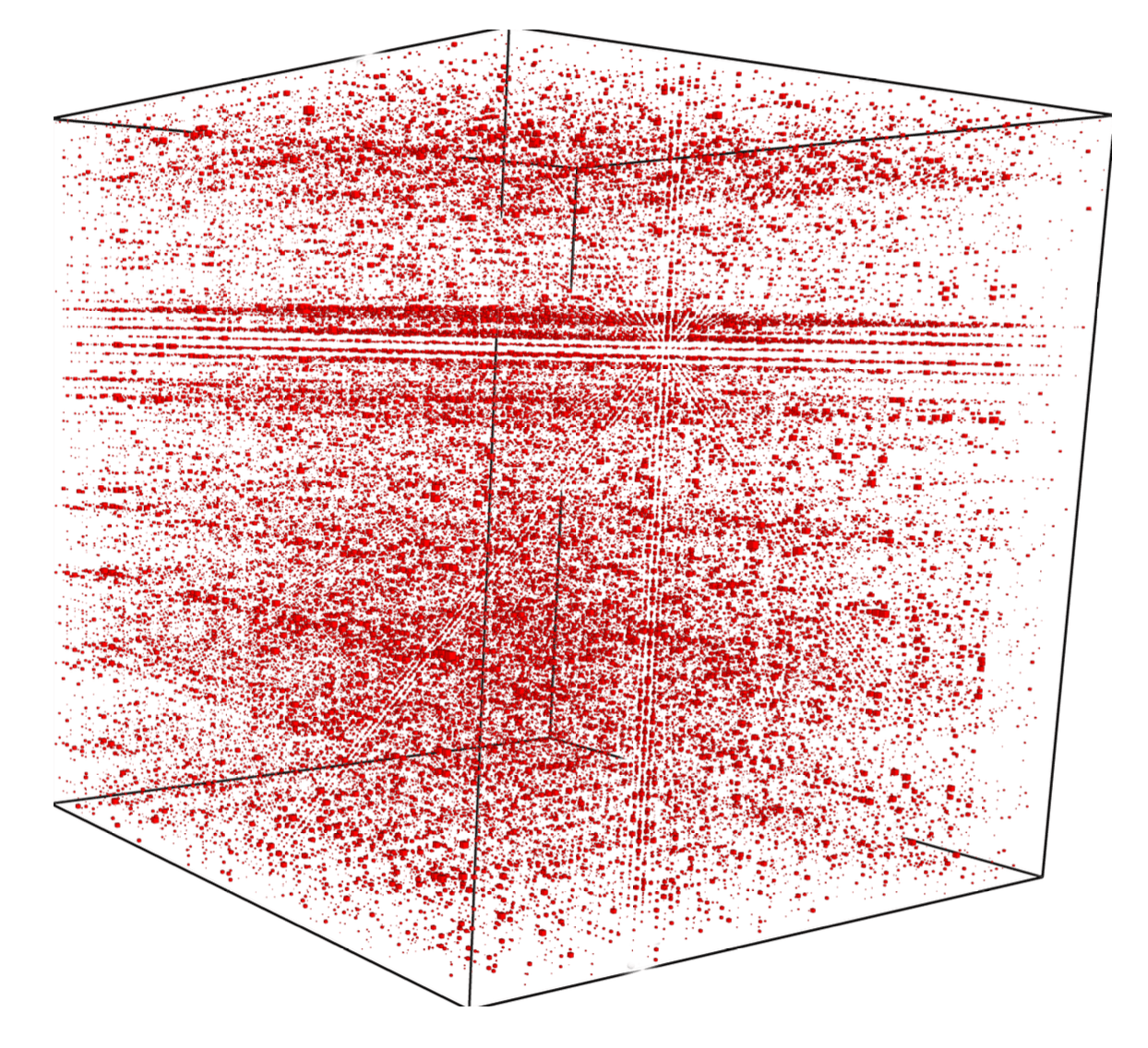
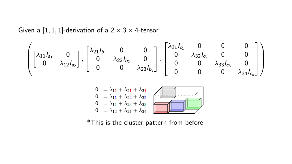
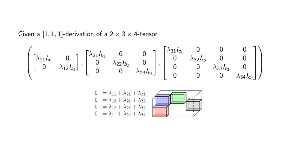
Recovery only up to level-sets in all three axes
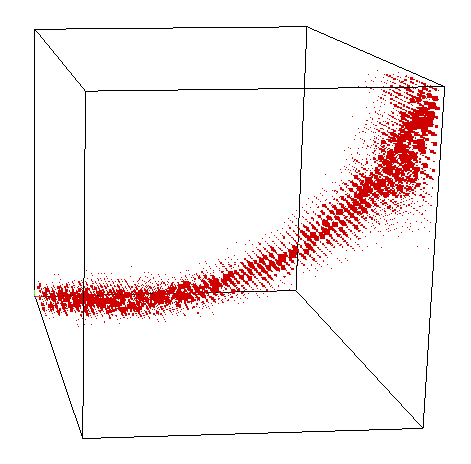
Recovery only up to level-sets in all three axes
Where is this coming from?
Stuff an infinite sequence
in a finite-dimensional space,
you get a dependence.
So begins the story of annihilator polynomials and eigen values.

An infinite lattice in finite-dimensional space makes even more dependencies.
(and the ideal these generate)
> M := Matrix(Rationals(), 2,3,[[1,0,2],[3,4,5]]);
> X := Matrix(Rationals(), 2,2,[[1,0],[0,0]] );
> Y := Matrix(Rationals(), 3,3,[[0,0,0],[0,1,0],[0,0,0]]);
> seq := [ < i, j, X^i * M * Y^j > : i in [0..2], j in [0..3]];
> U := Matrix( [s[3] : s in seq]);
        i   j   X^i * M * Y^j
        0   0   [ 1, 0, 2, 3, 4, 5 ]
        1   0   [ 1, 0, 2, 0, 0, 0 ]
        2   0   [ 1, 0, 2, 0, 0, 0 ]
        0   1   [ 0, 0, 0, 0, 4, 0 ]
        1   1   [ 0, 0, 0, 0, 0, 0 ]
        2   1   [ 0, 0, 0, 0, 0, 0 ]
        0   2   [ 0, 0, 0, 0, 4, 0 ]
        1   2   [ 0, 0, 0, 0, 0, 0 ]
        2   2   [ 0, 0, 0, 0, 0, 0 ]
        0   3   [ 0, 0, 0, 0, 4, 0 ]
        1   3   [ 0, 0, 0, 0, 0, 0 ]
        2   3   [ 0, 0, 0, 0, 0, 0 ]
In detail
Step out the bi-sequence
> E, T := EchelonForm( U );     // E = T*U
        0   0   [ 1, 0, 2, 3, 4, 5 ]    1
        1   0   [ 1, 0, 2, 0, 0, 0 ]    x
        0   1   [ 0, 0, 0, 0, 4, 0 ]    y
Choose pivots
Write null space rows as relations in pivots.
> A<x,y> := PolynomialRing( Rationals(), 2 );
> row2poly := func< k | &+[ T[k][1+i+3*j]*x^i*y^j :
     i in [0..2], j in [0..3] ] );
> polys := [ row2poly(k) : k in [(Rank(E)+1)..Nrows(E)] ];
        2   0   [ 1, 0, 2, 0, 0, 0 ]    x^2 - x
        1   1   [ 0, 0, 0, 0, 0, 0 ]    x*y
        2   1   [ 0, 0, 0, 0, 0, 0 ]    x^2*y
        0   2   [ 0, 0, 0, 0, 4, 0 ]    y^2 - y
        1   2   [ 0, 0, 0, 0, 0, 0 ]    x*y^2
        2   2   [ 0, 0, 0, 0, 0, 0 ]    x^2*y^2
        0   3   [ 0, 0, 0, 0, 4, 0 ]    y^3 - y
        1   3   [ 0, 0, 0, 0, 0, 0 ]    x*y^3
        2   3   [ 0, 0, 0, 0, 0, 0 ]    x^2*y^3
> ann := ideal< A | polys >;
> GroebnerBasis(ann);
    x^2 - x,
    x*y,
    y^2 - y
Take Groebner basis of relation polynomials
Groebner in bounded number of variables is in polynomial time (Bradt-Faugere-Salvy).

Same tensor,
different operators,
can be different annihilators.
Different tensor,
same operators,
can be different annihilators.

Data
Action by polynomials
Resulting annihilating ideal
Could this be wild? Read below.
Annihilators
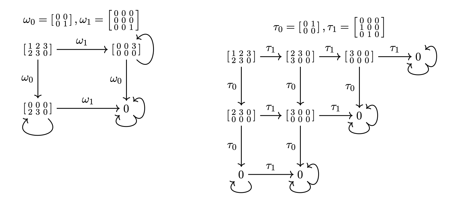


So given
- a tensor \(t\)
- a polynomial \(p(X)\)
- transverse operators \(\omega\)
\((\forall v)\,\langle t\mid p(\omega)\mid v\rangle=0\) just means \(p(X)\) is in the annihilator of this action.


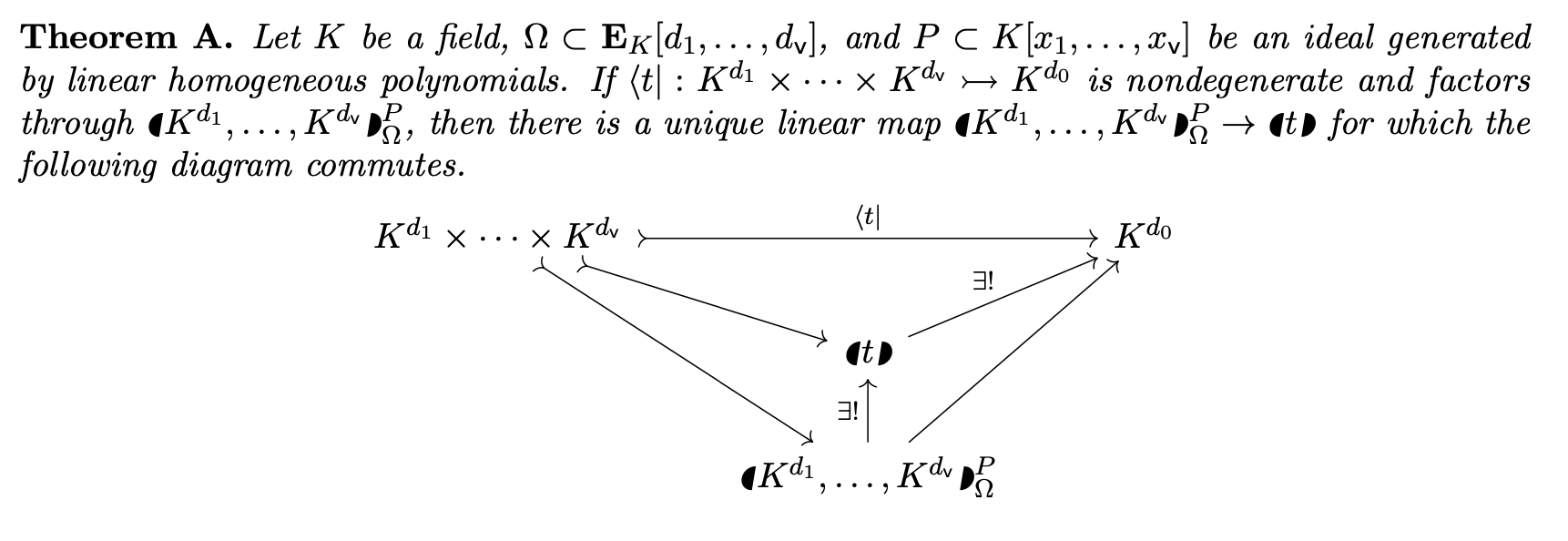
Controlling Conenction
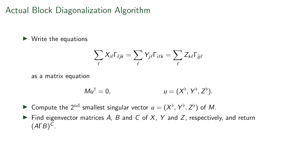
(First-Maglione-W.)
\(N(P,\Delta)=\{t\mid (\forall v)(\langle t\mid P(\Delta)|v\rangle=0)\}\) "closed" tensor space
\(I(S,\Delta)=\{p(X)\mid (\forall v)(\langle S\mid P(\Delta)|v\rangle=0)\}\) "closed" ideal
\(Z(S,P)=\{\omega\mid (\forall v)(\langle S\mid P(\omega)|v\rangle=0)\}\) "closed" scheme
Strategy
- tensors are the input data
- Polynomials are parameters we select
- Operator sets are what we want to explore our tensor
Summary of Trait Theorems (First-Maglione-W.)
- Linear traits correspond to derivations.
- Monomial traits correspond to singularities
- Binomial traits are only way to support groups.
For trinomial ideals, all geometries can arise so classification beyond this point is essentially impossible.
3 critically depends on Eisenbud-Sturmfels work on binomial ideals so it is restricted to vector spaces for now.
Derivations & Densors
Unintended Consequences
Since Whitney's 1938 paper, tensors have been grounded in associative algebras.
Derivations form natural Lie algebras.
If associative operators define tensor products but Lie operators are universal, who is right?
Tensor products are naturally over Lie algebras
Theorem (FMW). If
Then in all but at most 2 values of a
In particular, to be an associative algebra we are limited to at most 2 coordinates. Whitney's definition is a fluke.
Module Sides no longer matter
- Whitney tensor product pairs a right with a left module, often forces technical op-ring actions.
- Lie algebras are skew commutative so modules are both left and right, no unnatural op-rings required.
Associative Laws no longer
- Whitney tensor product is binary, so combining many modules consistantly by associativity laws isn't always possible - different coefficient rings.
- Lie tensor products can be defined on arbitrary number of modules - no need for associative laws.
Missing opperators
- Whitney tensor product puts coefficient between modules only, cannot operate at a distance.
As valence grows we act on a linear number of spaces but have exponentially many possible actions left out.
Lie tensor products act on all sides.
Densor
\((|t|):=N(x_1+\cdots+x_n,Z(t,x_1+\cdots+x_n))\)
Monomials, Singularities, & simplicial complexes

Shaded regions are 0.
Thm(FMW) Traits of operators that preserve a singularity have traits whose ideal is the Stanley-Reisner of complex.
Local Operators
I.e. operators that on the indices A are restricted to the U's.
Claim. Singularity at U if, and only if, monomial trait on A.
Singularities come with traits that are in bijection with Stanley-Raisner rings, and so with simplicial complexes.
Binomials & Groups
Theorem (FMW). For fields. If for every S and P
then \(\exists Q, Z(S,P)^{\times}=Z(S,Q)^{\times}\)
and \(\gcd\{e_1(a)+f_1(a),\ldots, e_m(a)+f_m(a)\}\in \{0,1\}\).
Converse holds if \(supp(e_1+\cdots +e_m)\cap supp(f_1+\cdots +f_m)=\emptyset\) even without conditions of a field. We speculate this is a necessary condition.
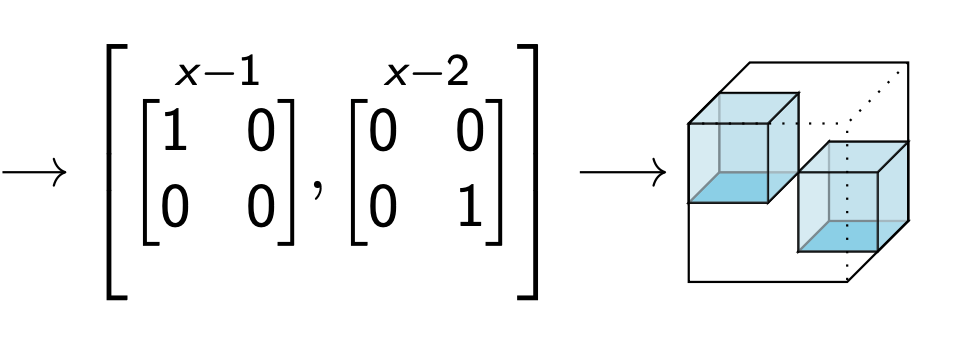
Back to decompositions
What are the markets?
Data table --> Multiplication table
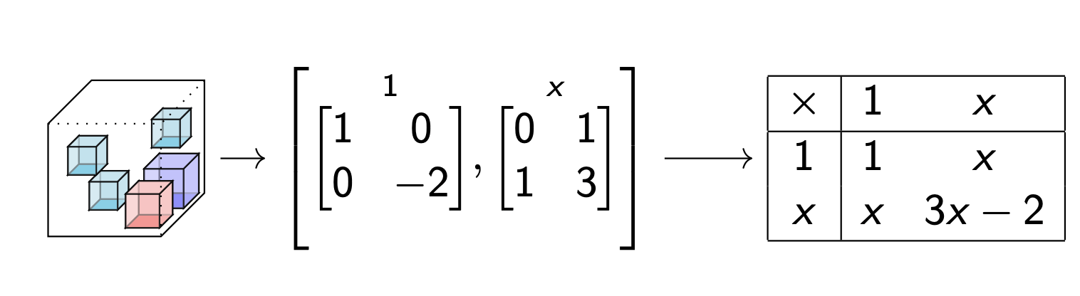
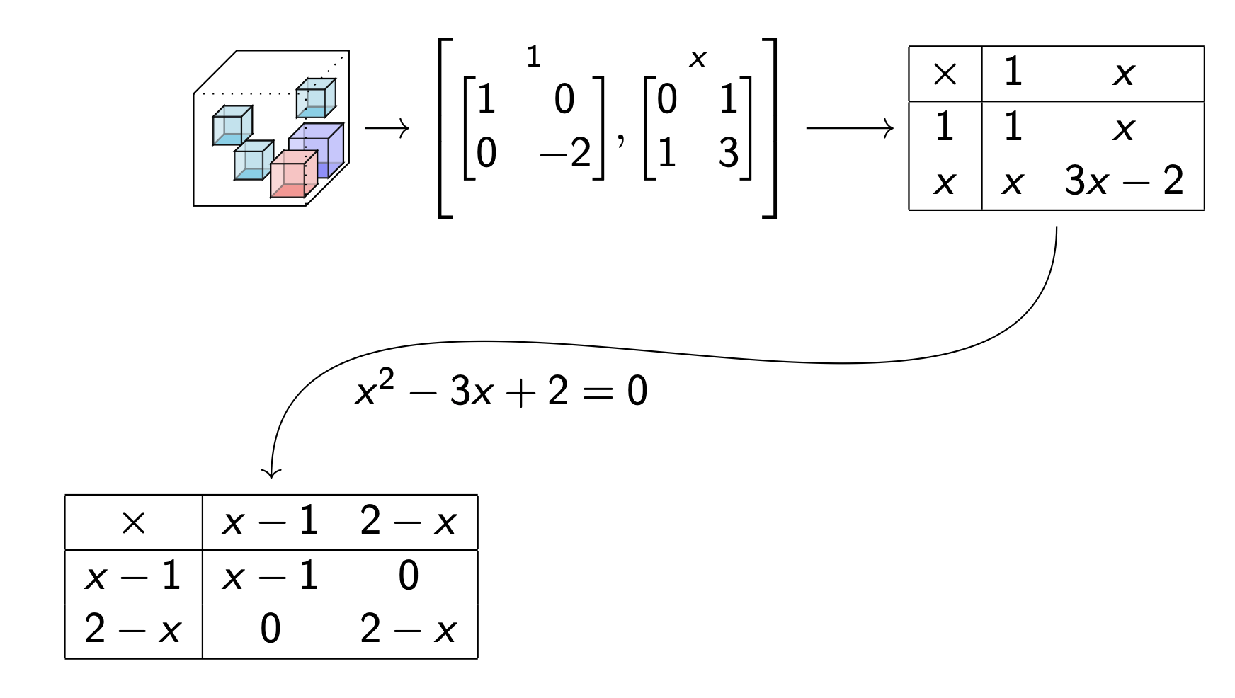
Use algebra to factor
Forcing Good Algebra in Real Life
In real life the "multiplication" you get from a tensor is bonkers!
\[*:\mathbb{R}^2\times \mathbb{R}^3\to \mathbb{R}^3\]
Get to 100's 1000's of dimensions and you have no chance to know this algebra.
Study a function by its changes, i.e. derivatives.
Study multiplication by derivatives:
\[\partial (f·g ) = (\partial f )·g + f·(\partial g ).\]
In our context discretized. I.e. ∂ is a matrix D.
\[D(f ∗g ) = D(f ) ∗g + f ∗D(g )\]
And it is heterogeneous, so many D's
\[D_0(f*g) = D_1(f)*g + f * D_2(g).\]
For general tensors \[\langle t| : U_{1}\times \cdots \times U_{\ell}\to U_0\] there are many generalizations.
E.g.
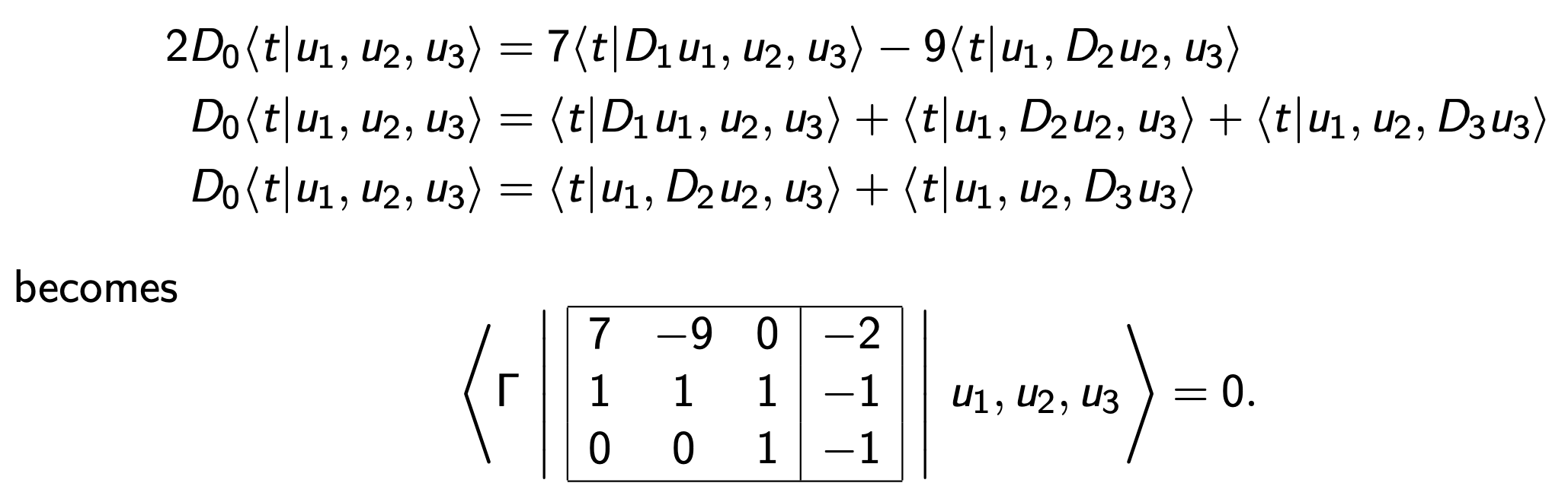
Or \[ D_0\langle t |u_1,u_2, u_3\rangle = \langle t| D_1 u_1, u_2,u_3\rangle + \langle t| u_1, D_2 u_2, u_3\rangle + \langle t|u_1, u_2, D_3 u_3\rangle.\]
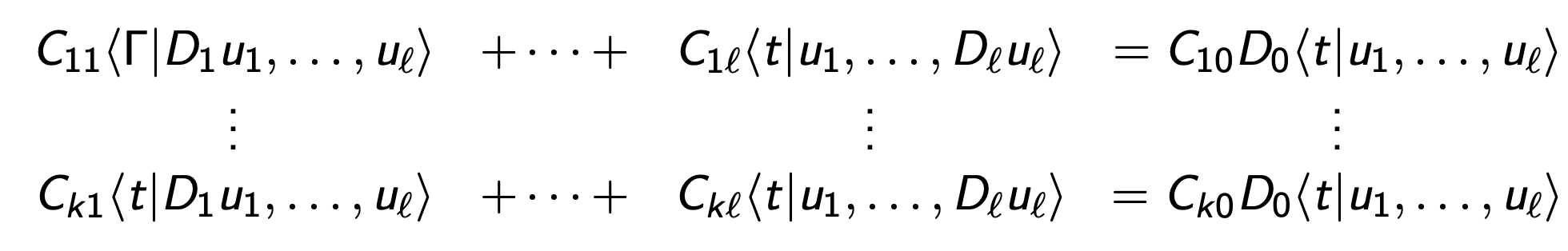
For general tensors \[\langle t| : U_{1}\times \cdots \times U_{\ell}\to U_0\]
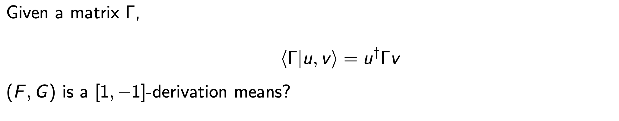
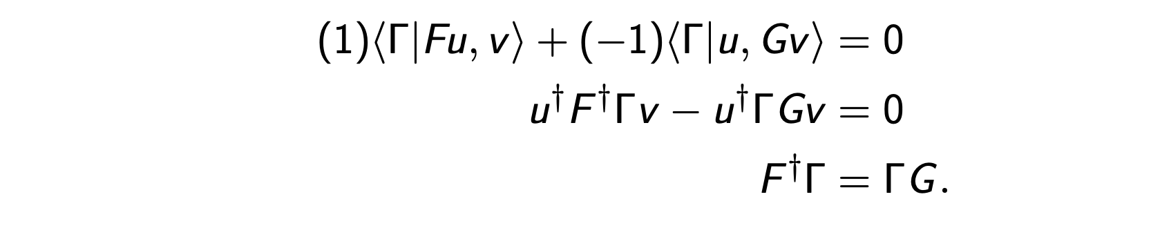
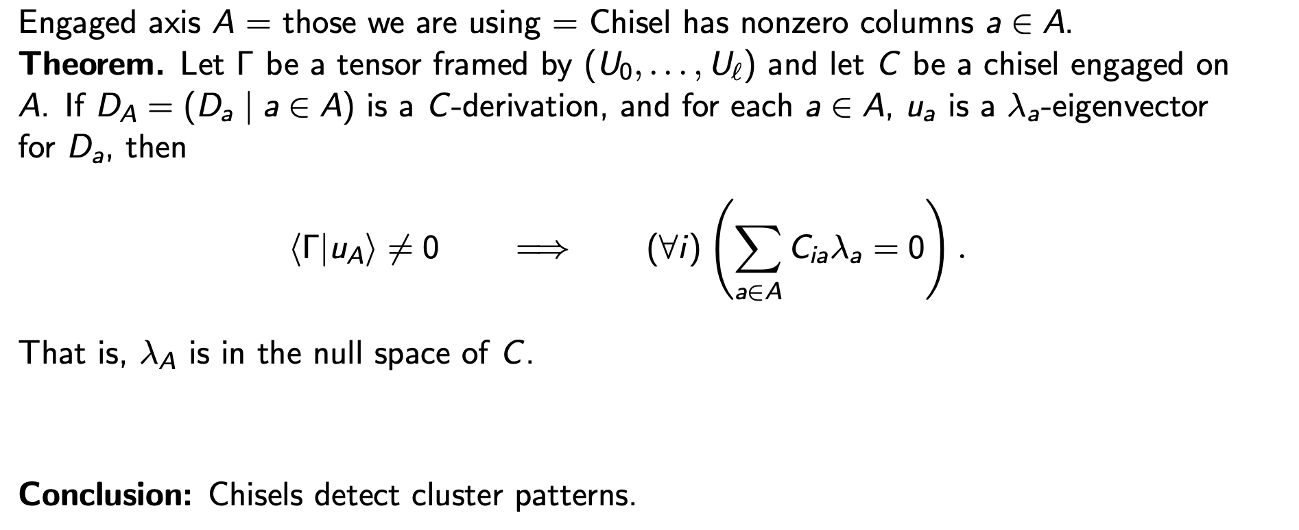
Choose a "chisel" (dleto) an augmented matrix C.
Write \[\langle \Gamma | C(D)|u\rangle =0\] to mean:
means chisel


And it's solutions are a Lie algebra
The main fact
Summary