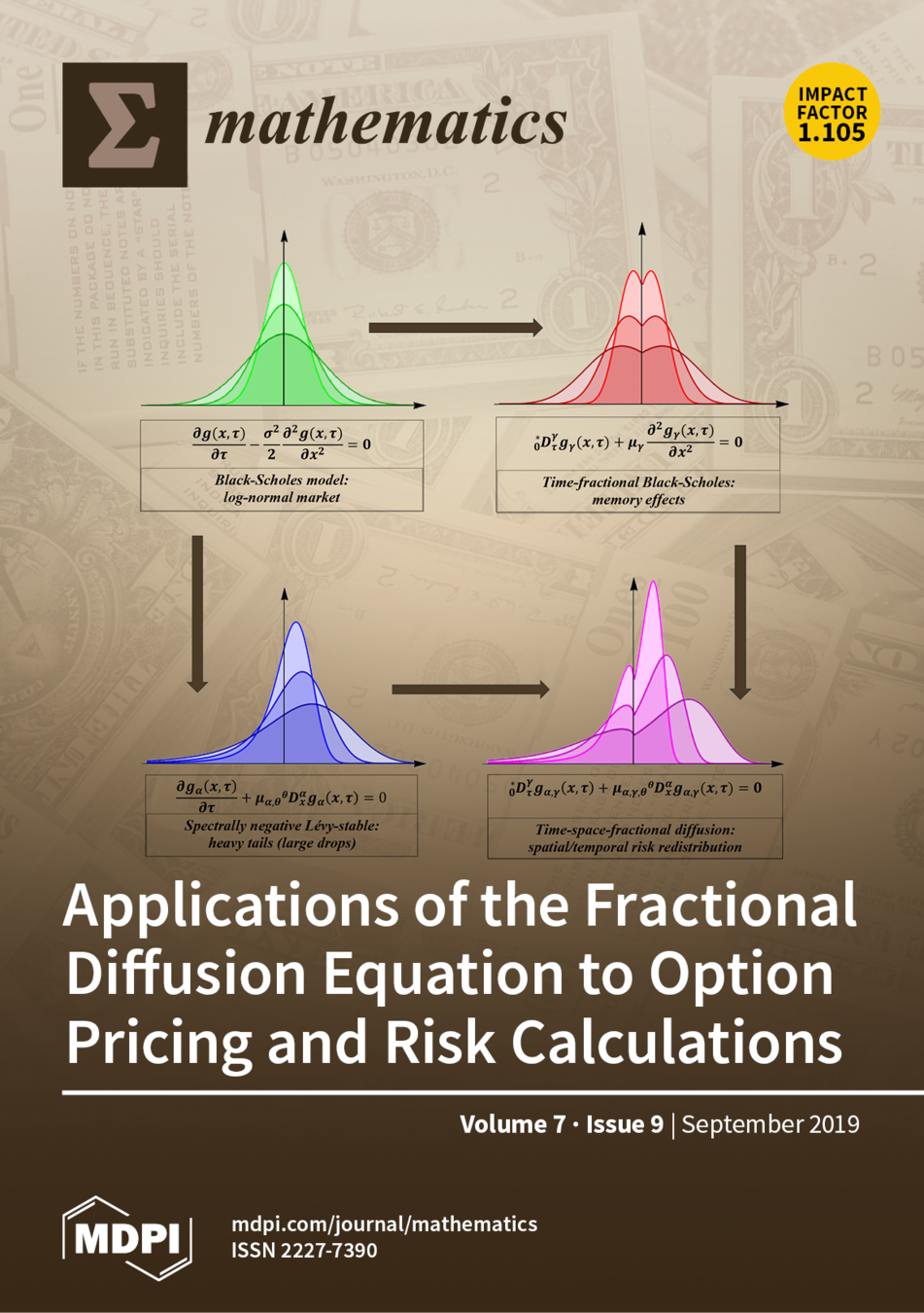
Applications of fractional diffusion in option pricing

Jan Korbel

Workshop Fractional Differential Equations, Applications and Complex Networks, Lorentz Center, Leiden

slides available at: slides.com/jankorbel

References:

[1] Physica A 449 (2016) 200-214; 10.1016/j.physa.2015.12.125

[2] Fract. Calc. Appl. Anal. 19 (6) (2016) 1414-1433; 10.1515/fca-2016-0073

[3] Fractal Fract. 2 (1) (2018) 15; 10.3390/fractalfract2010015

[4] Fract. Calc. Appl. Anal. 21 (4) (2018) 981-1004; 10.1515/fca-2018-0054

[5] Risks 7 (2) (2019) 36; 10.3390/risks7020036

[6] Mathematics 7 (9) (2019) 796; 10.3390/math7090796

[7] Fract. Calc. Appl. Anal. 23 (4) (2020) 996-1012; 10.1515/fca-2020-0052

[8] Risks 8 (4) (2020) 124; 10.3390/risks8040124

[9] Mathematics 9(24), 3198;10.3390/math9243198

Work [2] has been first discussed with Yuri Luchko here

more than 7 years ago

Review paper [6]

Recent paper [7] with Živorad and Johan

Option pricing

• First option pricing model (Black and Scholes 1973) 
  • based on ordinary Brownian motion
  • Nobel prize in economics (Scholes, Merton) - 1997
• ​In financial crises or in complex markets, the model cannot catch
  realistic market dynamics
  • large drops, sudden shocks, memory effects
• Finite moment log-stable model (Carr and Wu 2003)
  • based on Lévy-stable fractional diffusion
  • enables large drops
• We generalize the models by using space-time fractional diffusion equation

Space-time fractional diffusion 

The STFD equation is defined as

$$ \left({}^*_0 \mathcal{D}^\gamma_t - \mu \ {}^\theta \mathcal{D}_x^{\alpha}\right) g(x,t) = 0$$

Caputo derivative: \( {}^*_{t_0} \mathcal{D}^\gamma_t f(t) = \frac{1}{\Gamma(\lceil \gamma \rceil - \gamma)} \int_{t_0}^t \mathrm{d} \tau \frac{f^{\lceil \gamma \rceil}(\tau)}{(t-\tau)^{\gamma + 1 - \lceil \gamma \rceil}}\)

Riesz-Feller derivative: \(\mathcal{F}[{}^{\theta} \mathcal{D}^\alpha_x f(x)](k) = -|k|^\alpha e^{i \, \mathrm{sign}(k) \theta \pi/2} \mathcal{F}[f(x)](k) \)

Solution can be defined in terms of Mellin-Barnes transform

$$g_{\alpha,\theta,\gamma}(x,t) = \frac{1}{2 \pi i} \frac{1}{\alpha x} \int_{c-i \infty}^{c+i \infty} \frac{\Gamma(\frac{y}{\alpha}) \Gamma(1-\frac{y}{\alpha})\Gamma(1-y)}{\Gamma(1-\frac{\gamma}{\alpha} y)\Gamma(\frac{\alpha-\theta}{2 \alpha} y) \Gamma(1- \frac{\alpha-\theta}{2 \alpha} y)} \left(\frac{x}{-\mu t}\right)^y \mathrm{d} y$$

[1] Physica A 449 (2016) 200-214

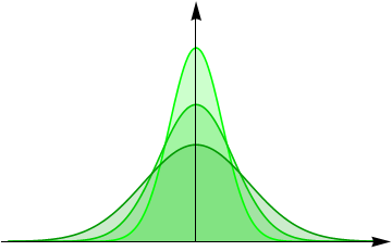
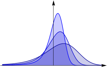
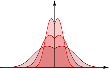
Space-time fractional diffusion 

• \(\gamma=1, \alpha=2\) - ordinary Gaussian diffusion

• \(\gamma=1, \alpha<2\) - Lévy-stable diffusion

• \(\gamma \neq 1, \alpha=2\) - diffusion with memory

• \(\gamma \neq 1, \alpha<2\) - space-time fractional diffusion

[6] Mathematics 7 (9) (2019) 796

Space-time fractional option pricing

Price of European call option: $$C(S,K,\tau) = \int_{-\infty}^\infty \max\{S e^{(r+\mu) \tau + x}-K,0\} g_{\alpha,\theta,\gamma}(x,\tau) \mathrm{d} x$$

Interpretation of parameters:

• \(\theta = \max\{-\alpha, \alpha-2\}\) 
  • maximally asymmetric distribution
  • power-law probability of drops (negative Lévy tail)
  •  Gaussian probability of rises (positive exponential tail
• \(\alpha < 2\) - risk redistribution to large drops
• \(\gamma \) - risk redistribution in time
  • \(\gamma < 1\) shorter contracts are more risky
  • \(\gamma > 1\) longer contracts are more risky

[1] Physica A 449 (2016) 200-214; [3] Fractal Fract. 2 (1) (2018) 15

Space-time fractional option pricing

We can rewrite the option price via Mellin-Barnes representation: $$C(S,K,\tau) = \frac{K e^{-r \tau}}{\alpha} \int_{c_1 - i \infty}^{c_1 + i \infty} \int_{c_2 - i \infty}^{c_2 + i \infty} (-1)^{t_2} \frac{\Gamma(t_2)\Gamma(1-t_2)\Gamma(-1-t_1+t_2)}{\Gamma(1-\frac{\gamma}{\alpha}t_1)}$$

$$\times(- \log\frac{S}{K}-(r+\mu) \tau)^{1+t_1-t_2}(-\mu\tau)^{-t_1/\alpha} \frac{\mathrm{d}t_1}{2\pi i}\wedge \frac{\mathrm{d} t_2}{2 \pi i}$$

This can be compactly represented as an integral over a complex differential 2-form:

$$C(S,K,\tau) = \frac{K e^{-r \tau}}{\alpha} \int_{\vec{c} + i \mathbb{R}^2} \omega$$

Its characteristic vector is \(\Delta = (-1+\frac{\gamma}{\alpha},1)\)

As a result, the integral can be expressed as a sum of residues, which can be simply written as a double sum

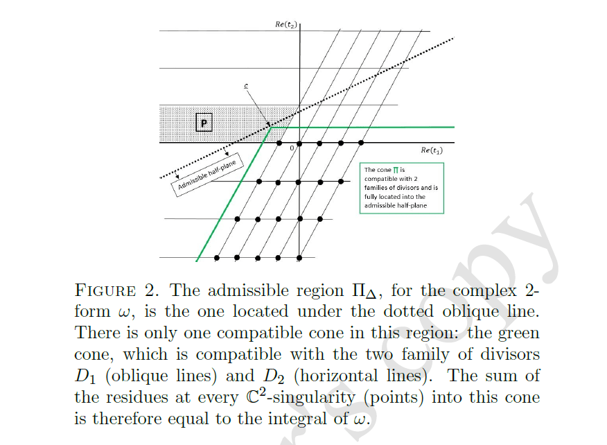
Residues of the differential 2-form

Double-series representation

By using residue summation in \(\mathbb{C}^2\) it is possible to express the price in terms of rapidly-convergent double series ( \(\mathcal{L} = \log \frac{S}{K} + r \tau\) ) 

$$C(S,K,\tau) = \frac{K e^{-r \tau}}{\alpha}  \sum_{n=0}^\infty \sum_{m=1}^\infty \frac{1}{n! \Gamma\left(1 + \frac{m-n}{\alpha}\right)}(\mathcal{L}+\mu \tau)^{n}(-\mu \tau)^{\frac{m-n}{2}}$$

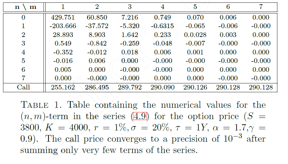
[4] Fract. Calc. Appl. Anal. 21 (4) (2018) 981-1004

• Pricing of more exotic types of options (American, digital,...) under the space-time fractional diffusion model and formulas for the risk sensitives  ("the Greeks" - Gamma, Delta, Rho,...)
  • [5] Risks 7 (2) (2019) 36; 10.3390/risks7020036
  • [6] Mathematics 7 (9) (2019) 796; 10.3390/math7090796

Space-time fractional option pricing

More results

Subordinator representation

\(g_{\alpha,\theta,\gamma}(x,t)\) can be represented as a subordinated process

$$g_{\alpha,\theta,\gamma}(x,t) = \int_0^\infty \mathrm{d} l K_\gamma(t,l) L_{\alpha}^\theta(l,x)$$

• \(L_{\alpha}^\theta(l,x)\) - Lévy-stable distribution with scaling parameter \(l\) 
• \(K_\gamma(t,l\) - subordinator (smearing kernel)
  • \(K_\gamma(t,l) =  \frac{t}{l^{1+1/\gamma} \gamma}  L_\gamma^{\gamma}\left(\frac{t}{l^{1/\gamma}}\right)\)
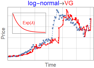
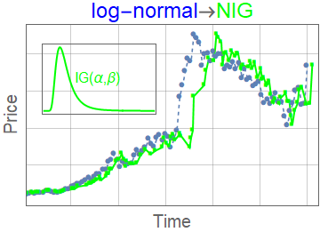
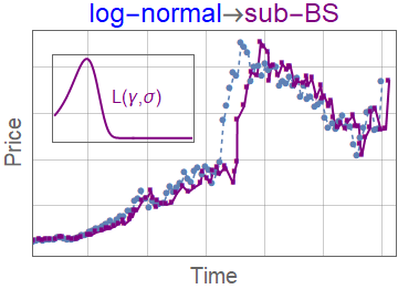
• We compare with other subordinated models
  • Variance gamma \(K_\lambda(t,l) =  \lambda  e^{\lambda  (-t/l)}\)
  • Negative inverse-gamma \(K_{\alpha,\beta}(t,l) = \frac{e^{-\frac{\beta }{t/l}} \left(\frac{\beta }{t/l}\right)^{\alpha }}{t/l \Gamma (\alpha )}\)

[1] Physica A 449 (2016) 200-214; [8] Risks 8 (4) (2020) 124

Subordinator representation

Space-time fractional option pricing with varying order of fractional derivatives

[3] FCAA 19 (6) (2016) 1414-1433 

• One of the important aspects of financial markets is switching between different regimes - conjuncture vs crisis
• Long-term scaling properties remain stable for each stock.
• This requires a time-dependent description by fractional diffusion of varying order.
•  Let us define intervals \(T_i = (t_i ; t_{i+1})\)
• Dynamics described by a space-time fractional diffusion in each interval $$ \left({}^*_{t_i} \mathcal{D}^{\gamma_i}_t - \mu \ {}^\theta \mathcal{D}_x^{\Omega \gamma_i}\right) g(x,t) = 0$$ with initial conditions: \(g_i(x,t_i) := g_{i-1}(x,t_i)\), \(g_0(x,0) := f(x)\)
• For \(\gamma_i > 1\) we add \(\frac{\partial g_i(x,t)}{\partial t} |_{t=t_i} = 0\)  
• The overall solution is given as a convolution $$g(x,t) = f(x) \star g_0(x,t_1-t_0) \star \dots \star g_i(x,t-t_i) \qquad \mathrm{for} \ t \in T_i$$

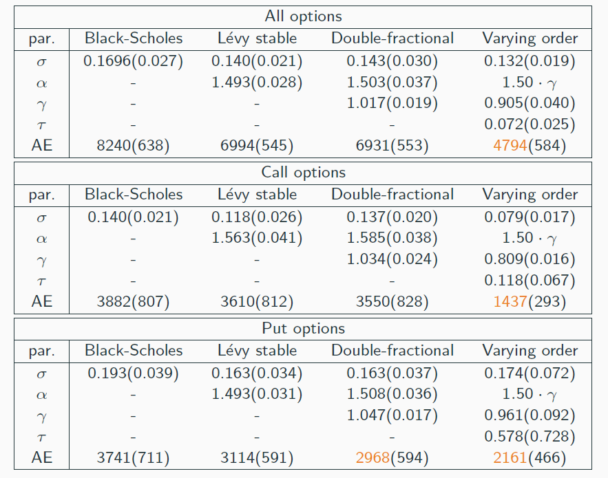
Space-time fractional option pricing with varying order of fractional derivatives

• The stable parameter is defined as \(\alpha_i = \Omega \gamma_i\) so that \(\Omega = \frac{\alpha_i}{\gamma_i}\) remains the same among all intervals \(T_i\) and characterizes the scaliung of \(g(x,t) \mathrm{d}{x} = \frac{1}{t^{\Omega}} g\left(\frac{x}{t^{\Omega}}\right) \mathrm{d}{x}\)
• Omega can be estimated e.g., from diffusion entropy analysis \(S(t) = - \int g(x,t) \ln g(x,t) = S(1) + \Omega \ln t\)
• This can be used, e.g., to model diffusion in a temporally abnormal period (crisis)
• We distinguish two intervals
  • short-term behavior affected by immediate dynamics
  • long-term behavior characterized by scaling properties

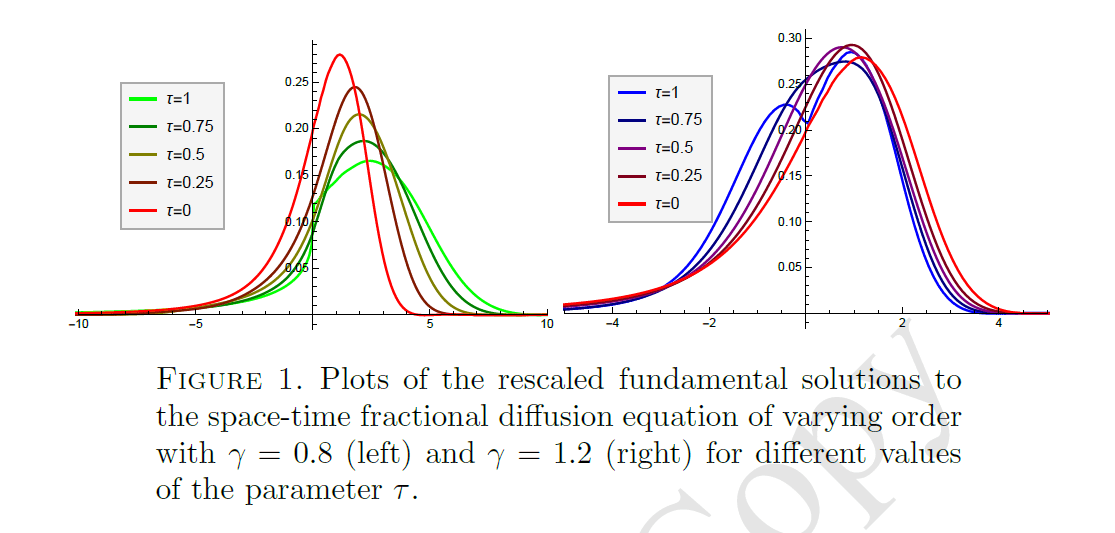
• This regime switch can be described by \(g(x, t)\)  as an overlap between space-time fractional
  diffusion (\(t \leq \tau\)  ) and Lévy flight (\tau \leq t).
• Considering \(\Omega\) as a system-characterized scaling exponent we obtain  $$g(x,t) = \left\{ \begin{array}{ll} g^{\theta}_{\Omega \gamma,\gamma}(x,t) & t \leq \tau \\ \left[ g^{\theta}_{\Omega \gamma,\gamma}(\tau) \star L_\Omega^\theta(t-\tau)  \right](x) & t > \tau \end{array}\right.$$ 

Space-time fractional option pricing with varying order of fractional derivatives

Space-time fractional option pricing with varying order of fractional derivatives

Applications of Hilfer-Prabhakar fractional diffusion to option pricing

[3] FCAA 23 (4) (2020) 996-1012 

• We also generalize the time-fractional derivative to a more generalized operator - Hilfer-Prabhakar derivative.
• We define the following functions:
• Generalized Mittag-Leffler function $$E^{\gamma}_{\rho,\mu}(t) := \sum_{k=0}^{\infty} \frac{\Gamma(\gamma+k)}{\Gamma(\gamma)\Gamma(\rho k + \mu)}t^k$$ 
• Rescaled GML function $$e^\gamma_{\rho,\mu,\omega}(t) := t^{\mu-1} E^{\gamma}_{\rho,\mu}(\omega t^\rho) $$
• Prabhakar integral $$(I^{\gamma}_{\rho,\mu,\omega,0+} f)(t) := \int_0^t (t-y)^{\mu-1} E^{\gamma}_{\rho,\mu}[\omega(t-y)^\rho]f(y) \mathrm{d} y$$

• Prabhakar derivative $$(D^{\gamma}_{\rho,\mu,\omega,0+} f)(x) := \frac{d^m}{d x^m}(I^{-\gamma}_{\rho,m-\mu,\omega,0+}f)(x)$$
• Generalized Hilfer-Prabhakar derivative $$(D^{\gamma,\mu,\nu}_{\rho,\omega,0+} f)(x):= (I^{-\gamma \nu}_{\rho,\nu(n-\mu),\omega,0+} \frac{\mathrm{d}^n}{\mathrm{d} x^n} I^{-(\gamma)(1-\nu)}_{\rho,(1-\nu)(n-\mu),\omega,0+} f)(x)$$
• The log-price evolution is then driven by the fractional diffusion equation $$D^{\gamma}_{\rho,\mu,\omega,0+} g(x,t) = \kappa \frac{\mathrm{d}^2}{\mathrm{d} x^2} g(x,t)$$
• The initial conditions are: \(u(x,0) = g(x)\), \(\frac{\partial u(x,t)}{\partial t} |_{t=0} = h(x)\)
• We can then calculate the value of the European call option if the underlying stock is driven by the aforementioned FDE

$$u(x,t) =c^+ u^+(x,t) \xi_{x\geq 0}(x)+c^- u^-(x,t) \xi_{x<0}(x)$$
$$u^+(x,t)=\sum_{n=0}^\infty  \Phi_{-2n}(x) (-\kappa)^n  e^{\gamma n}_{\rho,\mu n+1,\omega}(t)$$
$$u^-(x,t)=\sum_{n=0}^{\infty}\frac{|x|^{2n+1}}{(2n+1)!\kappa^{n+1}}{e}^{-\gamma(n+1)}_{\rho,-\mu(n +1)+1,\omega}(t)$$

The fundamental solution of the FDE:

Thus, the option price can be expressed as

$$C(S,K,\tau) = c^+ C^+(S,K,\tau) + c^- C^-(S,K,\tau)$$

$$ C^+(S,K,\tau)  =  \max\{S e^{(r+q)\tau}-K,0\} +  \phi_K(S e^{(r+q)\tau}) \sum_{n=1}^\infty (-\kappa)^n e^{\gamma n}_{\rho,\mu n+1,\omega}(\tau)$$

$$C^-(S,K,\tau) = \sum_{n=0}^{\infty}\frac{1}{(2n+1)!\kappa^{n+1}} {e}^{-\gamma(n+1)}_{\rho,-\mu(n+1)+1,\omega}(\tau)$$ $$ \times \left(e^{(r+q) \tau} \gamma(2(n+1),\log(Se^{(r+q)\tau}/K)) \frac{K \ (log(S e^{(r+q)\tau}/K))^{2(n+1)}}{2(n+1)} \right)$$
where \(\phi_K(x) = x\) if \(x > K\) and \(\phi_K(x) =0\) if \(x< K\), and \(\gamma\) is the incomplete gamma function.

Finally, we obtain that

Thank you!