From Spins to Society:
Modeling Collective Behavior
with Statistical Physics

Jan Korbel

CSH Winter School 2025
Slides available at: https://slides.com/jankorbel
Personal web: https://jankorbel.eu
Structure of this talk
This talk will consist of three parts:
1. Brief introduction to statistical physics
2. Statistical physics of spin systems
3. Statistical physics of social systems
The aim of this talk is to make an overview of models inspired by statistical physics in opinion dynamics models and other social models.
No prior knowledge of statistical physics is needed.
1. Brief introduction to statistical physics
From many to a few
- Most physical disciplines study the detailed prediction of physical systems, including their precise evolution in time
- They typically focus on systems composed of a few variables
- In physics, they are called degrees of freedom - DOF
- Examples of degrees of freedom:
- particle position \(x\)
- particle velocity \(v\)
- molecule angular momentum \(L\)
- For each degree of freedom, we have one (typically differential) equation that is interconnected with the other degrees of freedom
What if we have 1 mol (\(\approx 10^{23})\) particles?
Micro vs. Macro
For systems with a large number of DOF, it is typically not possible to get the exact microscopic description
- Too many equations to solve and too many details to be known
- The specific microscopic state is called the microstate
We typically do not need to know the exact microstate, we only want to know the specific macroscopic properties
- These macroscopic properties are called macrostates
- Statistical physics aims to provide a connection between microscopic and macroscopic description of systems

What is statistical physics?
The main concept is coarse-graining
Example: box of gas

position & velocity of each particle
(\(6 \times N_A \approx 10^{24} DOF)\)
volume, temperature, pressure
(a few thermodynamic variables)
Microscopic description
Classical mechanics (QM,...)
Mesoscopic description
Statistical physics
Macroscopic description
Thermodynamics
probability of measuring a particle
with given position and velocity
General description
Coarse-graining
\(\bar{X}= \frac{1}{n} \sum_i x_i\)

Coarse-graining = keeping the relevant information on a larger scale while omitting the details of the system
Example: dices
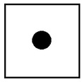
Consider dice with 6 states
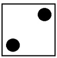
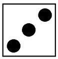
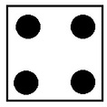
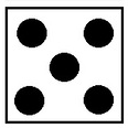
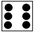
Let us throw a dice 5 times. The resulting sequence is
Microstate
How many times did a dice roll...
0
0
2
1
1
1
Mesostate
The average value is \(\bar{X} = 3.8\) Macrostate
Coarse-graining
Coarse-graining
# micro: \(6^5 =7776\)
# meso: \(\binom{6+5-1}{5} =252\)
# macro: \( 5\cdot 6-5\cdot 1 =25\)
Multiplicity W (sometimes \(\Omega\)):
# of microstates with the same mesostate
Question: how do we calculate multiplicity W for mesostate
1.) Permute all states
2.) Take care of overcounting
1.) Number of permutations: 5! = 120
2.) Overcounting - permutation of 2! = 2
Together: \(W(0,2,0,1,1,1) = \frac{5!}{2!} =60\)
0
0
2
1
1
1
Permutations:
1.
2.
3.
...
"General" formula - multinomials
$$W(n_1,\dots,n_k) = \left(\frac{\sum_{i=1}^k n_i}{n_1, \ \dots \ ,n_k}\right) = \frac{(\sum_{i=1}^k n_k)!}{\prod_{i=1}^k n_i!}= \frac{n!}{n_1! n_2! \dots n_k!}$$
for the case, when the individual dices are statistically independent, we end with a general formula for the multiplicity
From this, we can use the famous Boltzmann formula


Boltzmann's constant
\(k=1.380649 \times 10^{-23} J K^{-1}\)
Boltzmann-Gibbs-(Shannon) entropy
$$S = \log W \approx n\log n - n - \sum_{i} \left(n_i \log n_i - n_i \right)$$
Here, we use the normalization \(n = \sum_i n_i\)
and introduce probabilities \(p_i = n_i/n\)
$$ S = - n\sum_i p_i \log p_i$$
Finally the entropy per particle is
We use the Boltzmann formula (we set \(k_B = 1\) )
and Stirling's approximation \(\ln x! \approx x \ln x - x\)
We actually ended with the formula that is known as Shannon entropy in information theory
\( \mathcal{S} = S/n = -\sum_i p_i \log p_i \)
By using the relation \(n_i/n = p_i\), we actually used the law of large numbers. It says that for large \(n\), the relative frequency of an event converges to its probability, i.e.,
\(p_i = \lim_{n \rightarrow \infty} \frac{n_i(n)}{n}\)
This limit is in physics called thermodynamic limit.
Law of large numbers
What is actually \(p_i\)?
0
0
1
1
1
2
P( )=1/3
What is the meaning of entropy?
Properties of entropy:
- It is zero for certain events \(p = (1,0,\dots,0)\): \(S(p) = 0\) (\(1 \cdot \log 1 = 0 \cdot \log 0 = 0\))
- It is additive for independent events \(p_{ij} = p_i^{1} p_{j}^2\) $$S(p) = - \sum_{ij} p_{ij} \log p_{ij} = - \sum_{ij} p_{ij} \left(\log p_i^{1} + \log p_j^{2}\right)$$ $$ = -\sum_i p_i^{1} \log p_i^{1}-\sum_j p_j^{2} \log p_j^{2} = S(p^{1}) + S(p^{2})$$
- It is maximized by the uniform probability \(\max_p S(p) = \log n\) where \(p_{max} = \left(\frac{1}{n},\dots,\frac{1}{n}\right)\)
Thus, it measures the average amount of surprise (\(h_i=- \log p_i\))
when observing an event \(i\)
Entropy in statistical physicds
- Suppose now that we make a measurement of our system
- In our example of 5 dice, we observe that the average value of a dice is \(\bar{X} = 3.8\) (i.e., the total sum is 19)
- We now ask, what is the mesostate that corresponds to this measurement
0
0
2
1
1
1
Possible mesostates:
0
1
2
0
1
1
How many mesostates are there?
0
0
1
0
4
0
etc.
Intermezzo: Useful result from combinatorics
Bars & Stars theorems (|*)

Probability of a mesostate
- Here, the calculation is a bit more complicated since the (|*) theorem does not care that the maximum value on a dice is 6, so we have to exclude the cases that do not correspond to our example
- This can be solved by the so-called inclusion-exclusion principle, where we exclude unwanted cases
- After some algebra, the general formula gives us 17 distinct mesostates
We introduce the following notation:
0
0
1
1
1
\(=(6,5,4,2,2)\)
2
| (6,6,5,1,1) | (6,6,4,2,1) | (6,6,3,3,1) |
|---|---|---|
| (6,6,3,2,2) | (6,5,5,2,1) | (6,5,4,3,1) |
| (6,5,4,2,2) | (6,5,3,3,2) | (6,4,4,4,1) |
| (6,4,4,3,2) | (6,4,3,3,3) | (5,5,5,3,1) |
| (5,5,4,4,1) | (5,5,4,3,2) | (5,4,4,4,2) |
| (5,4,4,3,3) | (4,4,4,4,3) | (5,5,5,2,2) |
| (5,5,3,3,3) |
All mesostates with \(\bar{X} = 3.8\)
Q: What is the probability of observing such mesostate?
A: It is the multiplicity!
| W(6,6,5,1,1)=30 | W(6,6,4,2,1)=60 | W(6,6,3,3,1)=30 |
|---|---|---|
| W(6,6,3,2,2)=30 | W(6,5,5,2,1)=60 | W(6,5,4,3,1)=120 |
| W(6,5,4,2,2)=60 | W(6,5,3,3,2)=60 | W(6,4,4,4,1)=20 |
| W(6,4,4,3,2)=60 | W(6,4,3,3,3)=20 | W(5,5,5,3,1)=20 |
| W(5,5,4,4,1)=30 | W(5,5,4,3,2)=60 | W(5,4,4,4,2)=20 |
| W(5,4,4,3,3)=30 | W(4,4,4,4,3)=5 | W(5,5,5,2,2)=10 |
| W(5,5,3,3,3)=10 |
$$W(n_1,\dots,n_k) = \frac{n!}{n_1! n_2! \dots n_k!}$$
Probability of state with constraint
P( )
- How do we now calculate the probability of observing a value, e.g., what is ?
- For each mesostate, we calculate a probability of throwing three:
| P3(6,6,5,1,1)=0 | P3(6,6,4,2,1)=0 | P3(6,6,3,3,1)=0.4 |
|---|---|---|
| P3(6,6,3,2,2)=0.2 | P3(6,5,5,2,1)=0 | P3(6,5,4,3,1)=0.2 |
| P3(6,5,4,2,2)=0 | P3(6,5,3,3,2)=0.4 | P3(6,4,4,4,1)=0 |
| P3(6,4,4,3,2)=0.2 | P3(6,4,3,3,3)=0.6 | P3(5,5,5,3,1)=0.2 |
| P3(5,5,4,4,1)=0 | P3(5,5,4,3,2)=0.2 | P3(5,4,4,4,2)=0 |
| P3(5,4,4,3,3)=0.4 | P3(4,4,4,4,3)=0.2 | P3(5,5,5,2,2)=0 |
| P3(5,5,3,3,3)=0.6 |
Probability of state with constraint
- Now the probability is simply a weighted average of probabilities for each mesostate, weighted by its multiplicity, i.e.,
$$P(\qquad) = \frac{\sum_{m_i} P_3(m_i) W(m_i)}{\sum_{m_i} W(m_i)} = \frac{113}{605} \approx 18.7\%$$
here \(m_i\) are the mesostates that satisfy the constraint
This is quite complicated!
But what happens if we increase the number of dice?
Will it get more complicated or easier?
What happens if we rescale the problem?
- Suppose now that we do not throw 5 dice, but 10 dice, while the average value is the same (\(\bar{X} =3.8\)).
- What happens to multiplicity?
- Let us start with the mesostates, which are just double the mesostates for five dice, i.e., $$ (6,6,5,1,1) \mapsto (6,6,6,6,5,5,1,1,1,1)$$
- Then, the multiplicity can be expressed as
$$W(2n_1,\dots,2n_k) = \frac{(2n)!}{(2n_1)! (2n_2)! \dots (2n_k)!}$$
| W2(6,6,5,1,1)=3150 | W2(6,6,4,2,1)=12600 | W2(6,6,3,3,1)=6300 |
|---|---|---|
| W2(6,6,3,2,2)=3150 | W2(6,5,5,2,1)=12600 | W2(6,5,4,3,1)=113400 |
| W2(6,5,4,2,2)=12600 | W2(6,5,3,3,2)=12600 | W2(6,4,4,4,1)=420 |
| W2(6,4,4,3,2)=12600 | W2(6,4,3,3,3)=420 | W2(5,5,5,3,1)=420 |
| W2(5,5,4,4,1)=6300 | W2(5,5,4,3,2)=12600 | W2(5,4,4,4,2)=420 |
| W2(5,4,4,3,3)=3150 | W2(4,4,4,4,3)=45 | W2(5,5,5,2,2)=210 |
| W2(5,5,3,3,3)=210 |
Let us denote \(W_2(n_1,\dots,n_k) = W(2n_1,\dots,2n_k)\)
Multiplicities for double-configurations
What happens to the multiplicities?
Note: there are also other mesostates that are not double-configurations
Thermodynamic limit
- By rescaling the system, the most probable mesostates are observed much more often than the rest of the mesostates
- In thermodynamics, we are dealing with a large number of DOF (imagine \(10^{23}\) dice )
- As a consequence, only the mesostate with the largest multiplicity becomes relevant; all others become negligible
- How do we calculate the state with maximum multiplicity?
- We maximize the entropy (log of multiplicity) with respect to given constraints
Maximum entropy principle
- We define a probability \(p_i\) of a state \(\epsilon_i\)
- We maximize the entropy \(S=- \sum_i p_i \log p_i\) with constraints on
- normalization \(\sum_i p_i =1\)
- average outcome \(E = \sum_i p_i \epsilon_i\)
- This can be done by the methods of Lagrange multipliers
- We define the function \(L\) such that $$L = S(p) - \alpha \left(\sum_i p_i-1\right) - \beta \left(\sum_i p_i \epsilon_i - E\right)$$
- The maximum can be calculated from the condition \(\frac{\partial L}{\partial p_i} = 0\): $$- \log p_i - 1 - \alpha - \beta \epsilon_i = 0$$
- We obtain that \(p_i = \exp(-1-\alpha-\beta \epsilon_i) \)
Maximum entropy principle
- From the normalization constraint, we obtain that $$\exp(\alpha+1) = \sum_i \exp(-\beta \epsilon_i) \equiv Z$$ and therefore we finally obtain the form of the MaxEnt distribution:
$$p(\epsilon_i) = \frac{1}{Z} \exp(-\beta \epsilon_i)$$
It is called Boltzmann distribution and Z is called partition function
The entropy is then $$S = -\sum_i p(\epsilon_i) \log p(\epsilon_i) = -\sum_i p(\epsilon_i) \left(- \beta \epsilon_i - \ln Z\right) = -\beta E - \ln Z$$
The Lagrange parameter \(\beta\) has to be determined from energy constraint
$$\sum_i \epsilon_i \frac{\exp(-\beta \epsilon_i)}{Z(\beta)} = E$$
Example: MaxEnt distribution of dices
- Let us now exemplify the MaxEnt distribution on our example of dice
- The probability distribution is $$p(x) = \frac{\exp(-\beta x)}{Z}$$
- The Lagrange parameter \(\beta\) has to calculated from $$ \sum_{x=1}^6 x \frac{\exp(-\beta x)}{Z} = 3.8$$
- By solving this equation numerically, we obtain \(\beta = -0.1035\)
- Probabilities are:
- \(p(1) = 0.1267\)
- \(p(2) = 0.1405\)
- \(p(3) = 0.1558\)
- \(p(4) = 0.1728\)
- \(p(5) = 0.1917\)
- \(p(6) = 0.2126\)
Thermodynamic interpretation
- So far, we have not been connecting our findings with thermodynamics (or physics at all)
- Let us now make use of the properties of the entropy
- We show that the Boltzmann distribution has unique properties
- We also discuss the meaning of parameter \(\beta\)
- Consider a system composed of two subsystems \(A\) and \(B\)

The total energy of joint system \(A+B\) is conserved.
Thermodynamic equilibrium
- We know that the entropy of two statistically independent systems is a sum of them: \(S_{A+B} = S_{A}+S_{B}\)
- The total energy is also a sum of energies:\(E = E_A + E_B\)
- Therefore we can write $$S_{A+B}(E) = S_A(E_A) + S_B(E_B)$$
- From the Maximum entropy principle, we obtain that $$\frac{\partial S_{A+B}}{\partial E_A}=0$$
- This leads to $$\frac{\partial S_A(E_A)}{\partial E_A} + \frac{\partial S_B(E_B)}{\partial E_A}= 0$$ $$\frac{\partial S_A(E_A)}{\partial E_A} - \frac{\partial S_B(E_B)}{\partial E_B}= 0$$
- Using the relation between entropy and energy, we obtain \(\beta_A = \beta_B\)
- This is the zeroth law of thermodynamics, where \(\beta = \frac{1}{k T}\)
Free energy and thermodynamic potentials
- Let us now have a look at the partition function
- From the relation between the entropy and energy we get $$ -k T \ln Z = E - T S \equiv F $$
- Here \(F\) is the so-called Helmholtz free energy
- Calculating the partition function gives us all the relevant information about the system:
$$U = k T^2 \frac{\partial \ln Z}{\partial T}$$
$$F = - k T \ln Z$$
$$S = -\frac{\partial F}{\partial T}$$
2. Statistical physics
of spin systems
The simplest example of a thermodynamic model
- One of the best-studied class of models in statistical physics are spin models
- Although their definition is very simple, they exhibit very complex and interesting phenomena
- They find applications in many fields, including neural networks (Hopfield model), opinion dynamics, epidemiology or computation
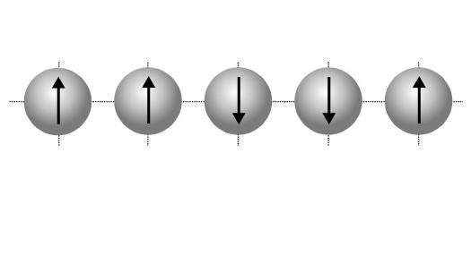
- In its simplest form, a spin model consists of N particles; each particle has two states: ↑ and ↓.

Ising model
- Probably the simplest spin model is the Ising model
- It was formulated first by Wilhelm Lenz (1920)
- It was first solved in 1D by Ernst Ising (1925)
- It is now 100 years anniversary
- In 2D, it was solved later by Lars Onsager
- We define the spins to have binary values \(\sigma_i = \{-1,+1\}\)
- The energy of the Ising model can be expressed as $$H(\sigma) = - J \sum_{\langle i j \rangle} \sigma_i \sigma_j - h \sum_i \sigma_i$$ where \(\langle i j \rangle\) denotes that we sum over \(i\) and \(j\) that are neighbors, \(J>0\) is the coupling constant and \(h\) is the external field
Ising model in 1D
- Let us start from the simplest Ising model: an Ising model on a one-dimensional chain
- The Hamiltonian simplifies to $$H(\sigma) = - J \sum_{i=1}^{N-1} \sigma_{i} \sigma_{i+1} - h \sum_i \sigma_i$$
- Let us take, for simplicity, \(h=0\) and calculate the partition function $$Z = \sum_{\sigma_i = \pm 1} \exp(-\beta J \sum_{i=1}^{N-1} \sigma_i \sigma_{i+1})= \sum_{\sigma_i=\pm 1} \prod_{i=1}^{N-1} \exp(-\beta J \sigma_i \sigma_{i+1})$$ $$= \prod_{i=1}^{N-1} \sum_{\sigma_i,\sigma_{i+1} = \pm 1} \exp(-\beta J \sigma_i \sigma_{i+1})=\prod_{i=1}^{N-1} \left[\exp(-\beta J)+\exp(\beta J)\right]$$ $$=\left[ 2\cosh(\beta J)\right]^{N-1}$$
Average magnetization
- Average magnetization can be just expressed as
$$m= \langle \sigma_i \rangle = \sum_{\sigma_i=\pm 1} \sigma_i \frac{\exp(-\beta H)}{Z}$$
- By analogous calculation, we can show that the average spin magnetization in 1D is zero.
- However, as we will see in the other models, in many spin systems, we observe the so-called spontaneous symmetry-breaking
- This means that while the magnetization is zero on the ensemble level, in one realization, we observe non-zero magnetization
- This can be examined by the correlations \(\langle \sigma_i \sigma_{i+k} \rangle\)
Ising model in 2D

- In this case, the Hamiltonian is the same, but just on a square lattice
- The solution of this model is possible, but it requires advanced methods like transfer matrix and theory of irreducible representation
- Interestingly, this model has a phase transition (so the phase diagram depends on a dimension)
- The critical temperature is $$T=\frac{2J}{k\ln(1+\sqrt{2})} \approx 2.269 \frac{J}{k}$$
Mean-field approximation of Ising model
- Although it might be quite difficult to get the exact solution for the Ising model, we might get a qualitative behavior by using the mean-field approximation
- We take the Hamiltonian $$H(\sigma) = - J \sum_{\langle i j \rangle} \sigma_i \sigma_j - h \sum_i \sigma_i$$ and rewrite the quadratic term with help of average magnetization \(m = \langle \sigma_i \rangle\) as $$\sigma_i \sigma_j = (\langle \sigma_i \rangle+ \delta \sigma_i) (\langle \sigma_j \rangle + \delta \sigma_j) $$ $$= \langle \sigma_i \rangle \langle \sigma_j \rangle + \delta \sigma_i \langle \sigma_j \rangle + \langle \sigma_i \rangle \delta \sigma_j + \delta \sigma_i \delta \sigma_j $$ where \(\delta \sigma_i\) is the difference from the mean magnetization
- If we assume that the differences are small, we can neglect the last term
Mean-field approximation of Ising model
- Theerefore, we can rewrite the quadratic term as $$\sigma_i \sigma_j \approx m (\sigma_i + \sigma_j) - m^2$$
- Consequently, the Hamiltonian can be rewritten as $$H^{MF}(\sigma) = \frac{kJ}{2} \sum_i (m^2-m 2\sigma_i)- h\sum_i \sigma_i$$ where \(k\) is the number of neighbors of \(i\) (also called node degree)
- Since the first term is a constant, we can omit it and end with the final Hamiltonian $$H^{MF}(\sigma) = -(J k m + h) \sum_i \sigma_i$$
- This is a large simplification because now each spin behaves independently from the other,s and the partition function can be decomposed into the product of one-particle partition functions $$Z(\sigma) = \prod_i Z(\sigma_i)$$
Mean-field approximation of Ising model
- The single-spin partition function is simple to calculate
$$Z(\sigma_i)=\sum_{\sigma_i=\pm 1}\exp(-\beta(J k m + h)\sigma_i)= \cosh(\beta( J k m + h)$$
- The total partition function is then simply \(\cosh(\beta J k m + h)^N\)
- There are various ways of calculating magnetization, but here we use the simplest one $$m = \langle \sigma_i \rangle = \sum_i \sigma_i p(\sigma_i) = p(\sigma_i=1)-p(\sigma_i=-1)$$
- By plugging in the Boltzmann distribution, we obtain $$m= \frac{\exp(\beta (J k m + h))- \exp(-\beta(J k m + h)}{Z}= \tanh(\beta J k m + h)$$
- Therefore, we obtain the self-consistency equation for \(m\), which tells us what \(m\) is allowable for which combination of parameters
Mean-field approximation of Ising model
- Let us focus on \(h=0\). The self-consistency equation \(m = \tanh(\beta_{eff} m)\) where \(\beta_{eff}=\beta J k\) has to be solved numerically.
- However, we can derive the critical temperature between the disordered phase (\(m=0\)) and the ordered phase (\(m \neq 0\)) by expanding the r.h.s. around \(m\) and obtain $$m \approx \beta_{eff} m - \frac{\beta_{eff}^3 m^3}{3} $$
- From this, we get that $$m\left( (1-\beta_{eff}) - \frac{\beta_{eff}^3}{3} m^2\right) = 0$$
- Therefore the solution is either \(m=0\) or $$m= \pm \sqrt{\frac{3(1-\beta_{eff})}{\beta_{eff^3}}}$$
- This solution is only possible for \(\beta_{eff} \geq 1\) which means \(T \leq J k \)
Phase-diagram

Ferromagnetic
Paramagnetic

Further examples of spin models
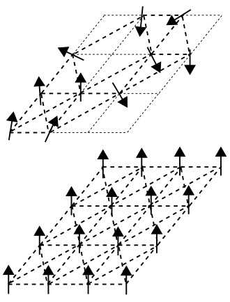
Ising antiferromagnetic model
- By allowing the coupling constant to be negative, the lowest energy state is when the neighboring particles have opposite spins
- This phase is called the antiferromagnetic phase
- Although the total magnetization is zero, we observe a distinct pattern of spins

ferromagnetic
antiferromagnetic
Further examples of spin models
Potts model
- In the Potts model, we allow spins to have multiple values, i.e., \(\sigma_i \in \{1,2,\dots,q\}\)
- The Hamiltonian is generalized so it favors aligned spins $$H(\sigma) = -J \sum_{\langle i j \rangle} \delta_{\sigma_i \sigma_j}$$
- For \(q=2\), we obtain the standard Ising model
- For \(q=3,4\), we obtain a second-order transition
- For \(q\geq 4\) we obtain a first-order transition
Further examples of spin models
XY model
- In this model, we now extend the spins into the 2-dimensional plane with unit size, i.e., they are on a unit circle \(\mathbf{\sigma}_i \in e^{i \theta_i}\)
- The Hamiltonian is the expressed as a scalar product $$H(\mathbf{\sigma}_i) = - J\sum_{\langle i j \rangle} \mathbf{\sigma}_i \cdot \mathbf{\sigma}_j = -J\sum_{\langle i j \rangle} \cos(\theta_i - \theta_j)$$
- It exhibits the Kosterlitz-Thouless transition (Nobel Prize 2000) between vortex and antivortex phases

Further examples of spin models
Spin glass model
- In this model, we now allow the coupling \(J\) to be both positive and negative in each link
- For each link, we model the coupling as a random quantity \(J_{ij} \sim N(J_0,J^2)\)
- The Hamiltonian is the expressed as$$H(\sigma_i,J_{ij}) = - \sum_{\langle i j \rangle} J_{ij}\sigma_i \sigma_j$$
- It exhibits the new phase called the frustrated (glassy) phase, where the temperature would normally allow to obtain the ordered (magnetic phase), but the couplings freeze the spins in irregular patterns, introducing local frustration (Nobel Prize 2021)
Monte Carlo simulations of Ising models
- In many cases, it is not possible to obtain exact analytic results
- In this case, we use the computer simulations
- The typical Monte Carlo simulation of spin systems:
0. - Initialize the system (assign the initial spins \(\sigma\))
1. - Randomly choose one spin \(\sigma_i\)
2. - Try to flip the spin \(\sigma_i^{'} = -\sigma_i\)
3. - Calculate the change in Hamiltonian \(\Delta H = H(\sigma^{'})-H(\sigma)\)
4. With probability \(p^{(ac)}(T,\Delta H)\), accept the flip,
otherwise, reject the flip
5. Repeat steps 1-4
Metropolis vs Glauber
There are two main types of acceptance criteria
- Metropolis algorithm: \(p^{ac}(T,\Delta E) = \min\{1,\exp(-\Delta E/T)\}\)
- Glauber dynamics: \(p^{ac}(T,\Delta E) = \frac{1}{1+\exp(\Delta E/T)}\)
- Since both algorithms fulfill the so-called detailed balance, they both converge to the correct equilibrium distribution
- The difference is how fast they converge
- Metropolis algorithm always accepts steps that decrease energy
- Glauber dynamics can be considered more physical
3. Statistical physics
of social systems
From spins to opinion
- In the dynamics of societies (regardless of whether on social networks or in real-life situations), there are a few mechanisms that drive the evolution of social systems
- The main concept of social dynamics is the presence of personal opinions or preferences
- Examples of opinions include:
- Political and voting preferences
- Policy adaptation (e.g., adaptation of a new technology)
- Product choice (Pepsi vs Coke, PC vs Mac)
- Cultural traits
- Opinions on other aspects
Types of opinions
Binary opinions
- Opinions take two values (e.g., YES/NO, left/right)
- It usually applies in bipartisan political systems or binary choice
- they can be modeled with a binary spin \(\sigma_i=\pm 1\)
- similar to Ising model
Types of opinions
Multistate opinions
- Opinions take multiple discrete values
- It usually applies in multi-partisan political systems or when multiple choices are available
- they can be modeled with a discrete spin \(\sigma_i\in \{1,2,\dots,k\}\)
- similar to Potts model
A
B
C
D
E
Types of opinions
Continuous opinions
- Opinions take continuous values (typically [-1,1] or [0,1])
- It usually applies to preference systems or sentiments
- they can be modeled with a continuous spin
- similar to various spin models (e.g., XY model)

-1
1
Driving mechanisms
Homophily
- "Birds of a feather flock together"
- People tend to like other peers with similar opinions
- For opinion vector \(\sigma = \{\sigma_1,\dots,\sigma_k\}\) the term \( \sum_i \sigma_i \sigma_i^{'}\) is larger the more opinions are the same
- Equivalent to the Ising model

Driving mechanisms
Bounded confidence
- Individuals adjust their opinions if they are sufficiently close to each other
- There is an interaction range where people tend to align
- We can express it by the Hamiltonian \(H(\sigma) = - \sum_{ij} J(\sigma_i,\sigma_j) \sigma_i \sigma_j\) where \(J(\sigma_i,\sigma_j) =1\) if \(|\sigma_i - \sigma_j| \leq \epsilon\) and 0 otherwise

Majority rule
- Individuals adopt the opinion of the majority in a group
- The update of the opinion can be expressed as \(\sigma = \max(\sigma^i | i \sim j)\) where \(i \sim j\) denotes all individuals that are neighbors of \(i\)
Driving mechanisms
Social pressure
- Individuals tend to follow the opinions of influencers (e.g., on social media)
- This can be modeled similarly to an external field in an Ising model $$H(\sigma) = - \sum_i h_i \sigma_i$$ where \(h_i\) denotes the strength of a social pressure
Driving mechanisms
Driving mechanisms
Heider balance
- "friend of my friend is my friend, enemy of my enemy is my friend"
- People tend to prefer balanced triangle relationships
- This can be modeled by considering the cubic Ising model on links $$H(J) = - \sum_{ijk} J_{ij} J_{jk} J_{ki}$$

Network topology
- The interaction between the individuals is taken on an underlying interaction networks, these include:

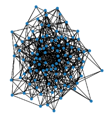


lattice
fully-connected
random
preferential attachment
small-world
Main phases of social systems
Cohesive phase
- The opinions are evenly spread on the network
- There is a consensus in the network
Main phases of social systems
Polarized phase
- The society gets polarized into two large groups
- There is no consensus in the network
Main phases of social systems
Fragmented phase
- Small groups are closed in echo chambers
- The communication between groups is suppressed
Overview of sociophysics models
Voter model
- In this simple model, the agents influence each other to change their opinions
- The simplest version of the model can be described as:
- 0. Initialize binary opinions \(\sigma_i \in \pm 1\)
- 1. Pick a voter uniformly at random \(\sigma_i\)
- 2. This voter adopts the state of a random neighbor \(\sigma_j\)
- 3. Repeat the steps 1. and 2. until a consensus is reached

Overview of sociophysics models
Voter model
- To mathematically express the update rule on a homogeneous graph, express the transition rate \(w_i\) at which voter state changes as \(w_i = \frac{1}{2} \left(1- \frac{\sigma_i}{k} \sum_{j: j \sim i} \sigma_j\right) \)
- The evolution of a spin can be expressed as \(\langle \dot{\sigma}_i \rangle = -2 \langle w_i \sigma_i\rangle\)
- Plugging into this, we get \(\langle\dot{\sigma}_i\rangle = -\langle\sigma_i \rangle + \frac{1}{k} \sum_{j: j \sim i} \langle \sigma_j \rangle\)
- By introducing average magnetization \(m = \frac{1}{N}\sum_i \langle \sigma_i \rangle\) we get \(\dot{m} =0\)
- There are many generalizations, as heterogeneous voters, confidence voting, heterogeneous networks, etc.

Overview of sociophysics models
Sznajd model
- The model is again an extension of Ising model
- It introduces the concept of social validation
- "United we stand, divided we fall"
- We start with chain of individuals with opinions $$\{\sigma_0,\sigma_1,\sigma_2,\dots,\sigma_N\}$$
- We randomly choose a pair of neigbors \(\{\sigma_i, \sigma_{i+1}\}\)
- If \(\sigma_i = \sigma_{i+1}\), then we make \(\sigma_{i-1} = \sigma_{i}\) and \(\sigma_{i+2} = \sigma_{i+1}\)
- If \(\sigma_{i} = - \sigma_{i+1}\), then we make \(\sigma_{i-1} = \sigma_{i+1}\) and \(\sigma_{i} = \sigma_{i+2}\)

Overview of sociophysics models
Sznajd model
- The solution of the evolution is two phases:
- Consensus (ferromagnetic phase)
- Stalemate (antiferromagnetic phase)
- Since the stalemate is not a very plausible state in social systems, several other generalizations have been proposed
Overview of sociophysics models
Axelrod model of culture dissemination
- In this model, the main aim is to study the dissemination of cultural traits in a multi-opinion society
- We assume that each individual has an opinion vector \(\sigma_i = \{\sigma_i^{(1)},\dots,\sigma_i^{(k)}\}\)
- In each step, we choose one individual at random \(i\) and one of its neigbors \(j\)
- The individual \(i\) interacts with their neigbor \(j\) with probability proportional to number of common opinions \(p = \frac{1}{k} \sum_{l=1}^k \delta(\sigma_i^{(l)},\sigma_j^{(l)})\)
- The interaction is the following: \(i\) adopts one opinion from the neigbor \(j\)
Overview of sociophysics models
Axelrod model of culture dissemination

Overview of sociophysics models
Social balance model
- This model is based on the Heider balance and the previously introduced Hamiltonian \(H = - \frac{J}{\binom{n}{3}} \sum_{ijk} J_{ij} J_{jk} J_{ki}\)
- This model shows the so-called rough energy landscape with many local minima that is hard to escape
- Therefore, the system can stuck in a frustrated state which is just a local minimum but not global minimum


Overview of sociophysics models
Social balance model
Overview of sociophysics models
Some work we do here at CSH
- In our models, we wanted to integrate the concept of homophily and Heider balance
- It turns out that Heider balance is just an emergent phenomenon that can be modeled with homophily
- We do it with the following Hamiltonian $$H(\sigma_i) = -\alpha \sum_{i,j:\mathrm{friends} } \sigma_i \sigma_j + (1-\alpha) \sum_{i,j: \mathrm{enemies} } \sigma_i \sigma_j$$
- Here, two neighbors are friends if they have more similar opinions than different ones
- \(\alpha\) determines how much we care about our friends versus our enemies
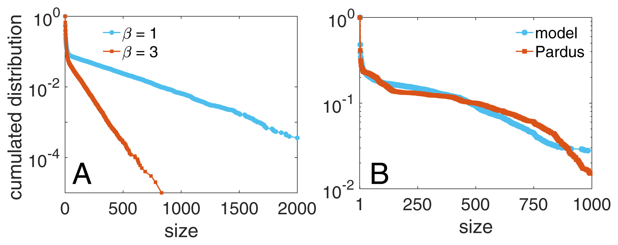
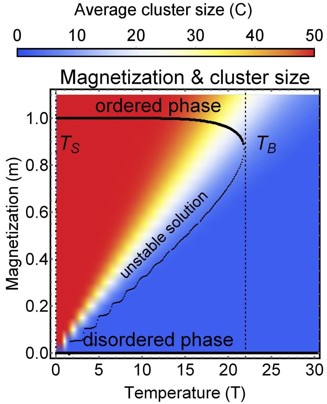
Group size distribution
Some work we do here at CSH - emergent balance
Overview of sociophysics models
The main idea: in large networks (like social networks) one cannot know all the relations between their friends
Overview of sociophysics models
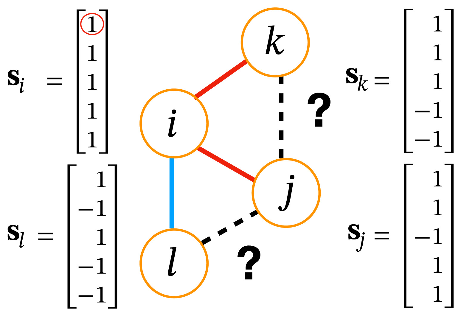
Some work we do here at CSH - group distribution
Hamiltonian of a group \(\mathcal{G}\)
\(H(\mathbf{s}_{i_1},\dots,\mathbf{s}_{i_k}) = \textcolor{red}{\underbrace{- \phi \, \frac{J}{2} \sum_{ij \in \mathcal{G}} A_{ij} \mathbf{s}_i \cdot \mathbf{s}_j}_{intra-group \ social \ stress}} \textcolor{blue}{ + \underbrace{(1-\phi) \frac{J}{2} \sum_{i \in \mathcal{G}, j \notin \mathcal{G}} A_{ij} \mathbf{s}_{i} \cdot \mathbf{s}_j}_{inter-group \ social \ stress}} \\ \qquad \qquad \qquad \qquad - \underbrace{h \sum_{i \in \mathcal{G}} \mathbf{s}_i \cdot \mathbf{w}}_{external \ field}\)
Group formation based on opinion= self-assembly of spin glass
Group 1
Group 2
friends
enemies
Theory
MC simulation
Overview of sociophysics models
Some work we do here at CSH - group distribution

Application online multiplayer game PARDUS