Motivation

System

heat bath

prepared at

 $T_1$

Typical experiment

heat bath

prepared at

 $T_2$

work reservoir

Typical experiment

$T$

$X$

$P(T)$

$X$

3rd trial

$T_3$

$X_3$

...

In reality

Measure a quantity $X$ and the temperature $T$

Temperature is measured with limited precision

In many experiments

• We do not know exact value of
  • amount of heat baths
  • temperatures
  • chemical potentials
  • energy spectrum
  • control protocol
  • transition rates
  • initial distribution

In real experiments, there is always some uncertainty about the system and its environment

Related approaches

Stochastic thermodynamics

Stochastic thermodynamics

1.) Consider linear Markov (= memoryless) with distribution $p_i(t)$.

Its evolution is described by the master equation

$$\dot{p}_t(x) = \sum_{x'} [K_{xx'} p_{t}(x') - K_{x'x} p_t(x) ]$$

$K_{xx'}$ is transition rate. 

2.) First law of thermodynamics - internal energy $U = \sum_x p(x) u(x)$ then First law of thermodyanmics is

$\dot{U} = \sum_x \dot{p}_t(x) u_t(x) + \sum_x p_t(x)  \dot{u}_t(x) = \dot{Q} + \dot{W}$

$\dot{Q}$ - heat rate

$\dot{W}$ - work rate

Stochastic thermodynamics

3.) Entropy of the system - Shannon entropy  $S = - \sum_x p_x \log p_x$. Equilibrium distribution is obtained by maximization of $S$ under the constraint of average energy 

$$\pi(x) = \frac{1}{Z} \exp(- \beta u(x)) \quad \mathrm{where} \ \beta=\frac{1}{k_B T}, Z = \sum_x \exp(-\beta u(x))$$

4.) Detailed balance - stationary state ($\dot{p}_t(x) = 0$ ) coincides with the equilibrium state $\pi(x)$. We obtain

$$\frac{K_{xx'}}{K_{x'x}} = \frac{\pi(x)}{\pi(x')} = e^{\beta(u(x') - u(x))}$$

Note: Transition rate satisfying LDB

a.) General form of transition matrix satisfying detailed balance

      Equilibrium distribution $\pi$:        $K \pi = 0$

      Define:                                            $\Pi := diag(\pi)$

      DB condition:                              $K \Pi = (K \Pi)^T$

      Decomposition:                             $K = R \Pi^{-1}$, $R$ - symmetric

      Normalization:                               $K = R \Pi^{-1} - diag (R \Pi^{-1} \cdot \mathbf{1})$

 b.) General form of transition matrix satisfying LDB

          $$K = \sum_{\nu=1}^N \left[ R^\nu (\Pi^\nu(\beta_\nu,\mu_\nu))^{-1} - diag (R^\nu \Pi^\nu(\beta_\nu,\mu_\nu))^{-1} \cdot \mathbf{1}\right]$$

Stochastic thermodynamics

5.) Second law of thermodynamics:

$$\dot{S} = - \sum_x \dot{p}_x \log p_x = \frac{1}{2} \sum_{xx'} \left[K_{xx'} p_t(x') - K_{x'x} p_t(x)\right] \log \frac{p_t(x')}{p_t(x)}$$

$$=\underbrace{\frac{1}{2} \sum_{xx'} \left[K_{xx'} p_t(x') - K_{x'x} p_t(x)\right] \log \frac{K_{xx'} p_t(x')}{K_{x'x} p_t(x)}}_{\dot{\Sigma}}$$ $$+ \underbrace{\frac{1}{2} \sum_{xx'} \left[K_{xx'} p_t(x') - K_{x'x} p_t(x)\right] \log \frac{K_{x'x}}{K_{xx'}}}_{\dot{\mathcal{E}}}$$

$\dot{\Sigma} \geq 0$  entropy production rate (2nd law of TD)

$\dot{\mathcal{E}} = \beta \dot{Q}$ entropy flow rate (connecting 1st and 2nd law quantities)

Stochastic thermodynamics

6.) Trajectory thermodynamics - consider stochastic trajectory

$\pmb{x}= (x_0,t_0;x_1,t_1;\dots)$. Energy $u_t(\pmb{x}) = u(\pmb{x}(t),\lambda(t))$

$\lambda(t)$ - control protocol

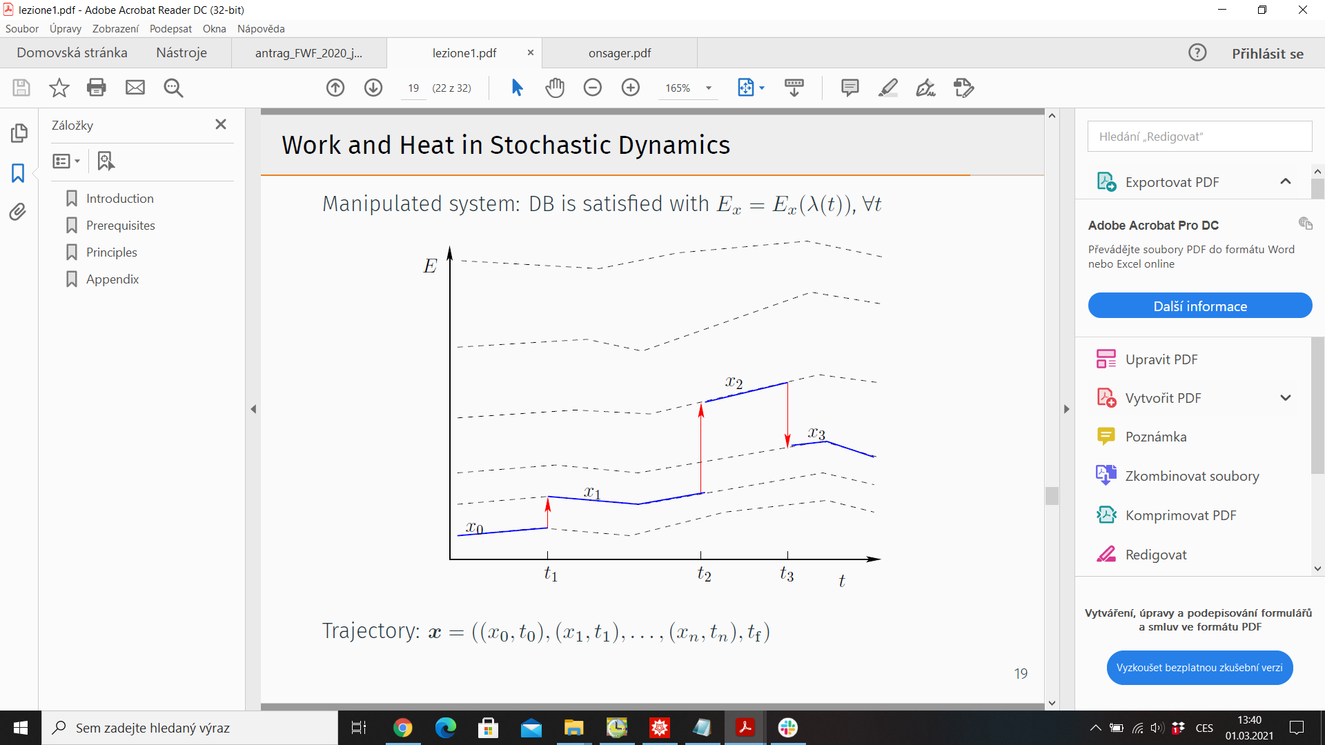
Probability of observing $\pmb{x}$: $\mathcal{P}(\pmb{x}$)

7.) Time reversal $\tilde{\pmb{x}}(t) = \pmb{x}(T-t)$

Reversed protocol $\tilde{\lambda}(t) = \lambda(T-t)$

Probability of observing reversed trajectory under reversed protocol $\tilde{\mathcal{P}}(\tilde{\pmb{x}})$

Stochastic thermodynamics

8.) Trajectory second law

Trajectory entropy: $s_t(\pmb{x}) = - \log p_t(\pmb{x}(t)$) 

Ensemble entropy: $S_t = \langle s_t(\pmb{x}) \rangle_{\mathcal{P}(\pmb{x})} = \int \mathcal{D} \pmb{x} \mathcal{P}(\pmb{x}) s_t(\pmb{x})$

Trajectory 2nd law $\Delta s =   \sigma +  \epsilon$

Trajectory EP: $\sigma = \underbrace{\ln p_t(\pmb{x}(t)) - \ln p_0(\pmb{x}(0))}_{\Delta s} + \underbrace{\sum_{i=1}^M \ln \frac{K_{\pmb{x}_{T_i}\pmb{x}_{T_{i-1}}}}{\tilde{K}_{\pmb{x}_{T_{i-1}}\pmb{x}_{T_i}}}}_{-\epsilon}$

Stochastic thermodynamics

9.) Detailed Fluctuation theorem

Relation to the trajectory probabilities

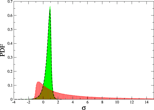
$$\log \frac{\mathcal{P}(\pmb{x})}{\tilde{\mathcal{P}}(\tilde{\pmb{x}})} =  \sigma$$

Detailed fluctuation theorem (DFT)

$$\frac{P(\sigma)}{\tilde{P}(-\sigma)} = e^{\sigma}$$

10.) Integrated fluctuation theorem 

By rearraning DFT we get $P(\sigma) e^{-\sigma} = \tilde{P}(-\sigma)$

By integrating over $\sigma$, we obtain IFT

$$\langle e^{- \sigma} \rangle = 1 \quad \stackrel{Jensen}{\Rightarrow} \langle \sigma \rangle =  \Sigma \geq 0$$

2nd law is consequence of FTs!

Stochastic thermodynamics in uncertain environment

Thermodynamics of systems coupled to uncertain environment

• Consider a set of apparatuses $\mathcal{A}$.
• For each apparatus $\alpha \in \mathcal{A}$, we have a system with a precise number of baths, temperatures, chemical potentials, etc. satisfying local detailed balance
• We consider a probability distribution $P^\alpha$ over the apparatuses

Effective value over the apparatuses can be defined as 

$$\overline{X}:= \int \mathrm{d} P^\alpha X^\alpha$$

Effective distribution $\bar{p}_x(t)$ fulfills the equation

  $\dot{\bar{p}}_x(t) = \sum_{x'} \int \mathrm{d} P^\alpha K^\alpha_{xx'} p^\alpha_{x'}(t)$   which is generally non-Markovian

Effective ensemble stochastic thermodynamics

• Expected internal energy is $\bar{U} = \int \mathrm{d} P^\alpha \sum_x p^\alpha_t(x) u^\alpha(x)$
• Expected first law of thermodynamics

$$\dot{\bar{U}} = \dot{\bar{Q}} + \dot{\bar{W}}$$

• Expected ensemble entropy $\bar{S} =  - \sum_x \int \mathrm{d} P^\alpha p_t^\alpha(x) \ln p_t^\alpha(x)$
• Expected second law of thermodynamics $$\dot{\bar{S}} = \dot{\bar{\Sigma}} + \dot{\bar{\mathcal{E}}}$$
• $\dot{\bar{\Sigma}} \geq 0$

• $\dot{\bar{\mathcal{E}}} = \overline{\beta \dot{Q}}$ - no explicit relation between $\dot{\bar{\mathcal{E}}}$ and $\dot{\bar{Q}}$

Effective trajectory stochastic thermodynamics

• Effective trajectory entropy is defined as $\overline{s}_t(\pmb{x}) = - \overline{\log p_t(\pmb{x}(t)}$)
• Ensemble average $\langle \overline{s}_t(\pmb{x})\rangle_{\overline{\mathcal{P}}(\pmb{x})} \neq \bar{S}_t \equiv \overline{\langle s^\alpha_t(\pmb{x}) \rangle_{\mathcal{P}^\alpha(\pmb{x})}}$
• In general, ensemble average and effective averaging do not commute
• As a consequence, the fluctuation theorems do not hold for $\overline{\sigma}$

Decomposition of effective EP

Denote $\mathcal{P}^\alpha(\pmb{x}) \equiv \mathcal{P}(\pmb{x}|\alpha)$ and $\mathcal{P}(\pmb{x},\alpha) = \mathcal{P}(\pmb{x}|\alpha) P^\alpha$

Effective ensemble EP $\bar{\Sigma}$ can be expressed as $$\bar{\Sigma} = \int \mathrm{d} P^\alpha \mathcal{D} \pmb{x} \, \mathcal{P}^\alpha(\pmb{x}) \sigma^\alpha(\pmb{x}) = \int \mathrm{d} \alpha \mathcal{D} \pmb{x} P^\alpha \mathcal{P}^\alpha(\pmb{x}) \ln \frac{\mathcal{P}^\alpha(\pmb{x}) P^\alpha}{\tilde{\mathcal{P}}^\alpha(\tilde{\pmb{x}}) P^\alpha}$$

$$= D_{KL}(\mathcal{P}(\pmb{x},\alpha)||\tilde{\mathcal{P}}(\tilde{\pmb{x}},\alpha))$$

By using chair rule for KL-divergence

$$D_{KL}(\mathcal{P}(\pmb{x},\alpha)||\tilde{\mathcal{P}}(\tilde{\pmb{x}},\alpha)) = D_{KL}(\mathcal{P}(\pmb{x})||\tilde{\mathcal{P}}(\tilde{\pmb{x}})) + D_{KL}(\mathcal{P}(\alpha|\pmb{x})||\tilde{\mathcal{P}}(\alpha|\tilde{\pmb{x}}))$$

where $\mathcal{P}(\pmb{x}) = \int \mathrm{d} \alpha \, P^\alpha \mathcal{P}(\pmb{x}|\alpha) \equiv \bar{\mathcal{P}}(\pmb{x})$ and $\mathcal{P}(\alpha|\pmb{x}) = \frac{\mathcal{P}(\pmb{x}|\alpha) P^\alpha}{\mathcal{P}(\pmb{x})}$

Phenomenological EP

Phenomenological EP $\underline{\Sigma} = D_{KL}(\mathcal{P}(\pmb{x})||\tilde{\mathcal{P}}(\tilde{\pmb{x}})) = \int \mathcal{D} \pmb{x} \mathcal{P}(\pmb{x}) \ln \frac{\mathcal{P}(\pmb{x})}{\tilde{\mathcal{P}}(\tilde{\pmb{x}})}$

Phenomenological trajectory EP is $\underline{\sigma} = \ln \frac{\mathcal{P}(\pmb{x})}{\tilde{\mathcal{P}}({\tilde{\pmb{x}}})}$

It is straightforward to show that $\underline{\sigma}$ fullfills detailed fluctuation theorem

$$\frac{P(\underline{\sigma})}{\tilde{P}(-\underline{\sigma})} = e^{\underline{\sigma}}$$

Phenomenological EP describes thermodynamics for the case of expected probability

It is a lower bound for the effective EP: $\overline{\Sigma} \geq \underline{\Sigma}$

Inference EP

Inference EP $\Omega = D_{KL}(\mathcal{P}(\alpha|\pmb{x})||\tilde{\mathcal{P}}(\alpha|\tilde{\pmb{x}})) = \int \mathrm{d} P^\alpha \mathcal{P}(\alpha|\pmb{x}) \ln \frac{\mathcal{P}(\alpha|\pmb{x})}{\tilde{\mathcal{P}}(\alpha|\tilde{\pmb{x}})}$

Inference trajectory EP as $\omega:= \sigma^\alpha - \underline{\sigma} =  \ln \frac{\mathcal{P}(\alpha|\pmb{x})}{\tilde{\mathcal{P}}(\alpha|\tilde{\pmb{x}})}$

We can also show that $\omega$ fulfills Detailed FT:

$$\frac{P(\omega|\pmb{x})}{\tilde{P}(-\omega|\tilde{\pmb{x}})} = e^{\omega}$$

From Integrated FT, we obtain that $\Omega_{\pmb{x}} = \langle \omega \rangle_{P(\omega|\pmb{x})} \geq 0$

Interpretation: $\Omega$ is the average rate of how much information we gain from Bayesian inference of $P(\alpha)$ from observing $\pmb{x}$

Interpretation of phenomenological EP

Let us consider $\pmb{x}_t$ as a part of trajectory $\pmb{x}$ from 0 to t.

Define $\underline{X}_t := \int \mathrm{d} \alpha  \mathcal{P}(\alpha|\pmb{x}_t) X^\alpha$

Then we can show that 

$$\underline{\sigma} = \underbrace{\ln \underline{p}_t(x(t)) - \ln \underline{p}_0(x_0)}_{\Delta \underline{s}} + \underbrace{\sum_{i=1}^M \ln \frac{\underline{K}_{\pmb{x}_{T_i}\pmb{x}_{T_{i-1}}}}{\tilde{\underline{K}}_{\pmb{x}_{T_{i-1}} \pmb{x}_{T_i}}}}_{-\underline{\epsilon}}$$ 

We can effectively treat the non-Markovian model with uncertain $\alpha$ as Markovian model with trajectory-dependent distribution $\mathcal{P}(\alpha|\pmb{x}_t)$

Example:

two-state system with uncertain temperature

Two-state CTMC with unknown temperature

$E_0$

$E_1$

consider $E_1 > E_0$

Consider transition rates:

$K_{0 \rightarrow 1} = e^{-\beta(E_0-E_1)/2}$

$K_{1 \rightarrow 0} = e^{-\beta(E_1-E_0)/2}$

The rates satisfy detailed balance

Let us assume that we do not know the inv. temperature $\beta$

Two-state CTMC with unknown temperature

We observe a trajectory $\pmb{x}$

According to the waiting times, we can calculate $\mathcal{P}(\beta|\pmb{x}_t)$ for times

$t = \{T_1,T_2,T_3\}$

Updating of $P(\beta) \mapsto P(\beta|\pmb{x}_t)$

from observing $\pmb{x}_t$

Text

True value: $\beta^\star = 1$

Updating of $P(\beta) \mapsto P(\beta|\tilde{\pmb{x}}_t)$

from reversed dynamics

Trajectory Inference EP

$\Omega_{\pmb{x}_t}$ increases in time

There is more!

• Maximal work extractions with uncertain temperatures
• Dynamic of the thermodynamic value of information                    

Possible extensions:

• Systems with uncertain energy spectrums
• Experiments with uncertain control protocols
• Complete analysis of maximal work extraction to reach a target distribution with a given probability measure, both when one can specify aspects of the evolution (e.g., a quenching Hamiltonian) and when  one can only specify it up to a given precision.

Thanks!