Lorenz Attractor in GeoGebra

First of all

First of all

we need to know the equations

\displaystyle\left\{ \begin{array}{rcl} \dfrac{dx}{dt}&=&\sigma (-x + y)\\ \\ \dfrac{dy}{dt}&=& -x z + \rho x - y \\ \\ \dfrac{dz}{dt}&=& x y - \beta z \end{array} \right.

System of differential equations

Lorenz system

\sigma\text{(sigma)}, \rho\text{(rho)},\text{ and } \beta\text{(beta)} \;\;\;\\ \text{are constants}
t
t
t
x
y
z
x
x
x
y
y
y
z
z
x

Non-linear system of

ordinary differential equations (ODEs)

Lorenz system

\sigma\text{(sigma)}, \rho\text{(rho)},\text{ and } \beta\text{(beta)} \;\;\;\\ \text{are constants}
\displaystyle\left\{ \begin{array}{rcl} \dfrac{dx}{dt}&=&\sigma (-x + y)\\ \\ \dfrac{dy}{dt}&=& -x z + \rho x - y \\ \\ \dfrac{dz}{dt}&=& x y - \beta z \end{array} \right.
t
t
t
x
y
z
x
x
x
y
y
y
z
z
x

Lorenz system

\(\dfrac{dx}{dt}=x'\)

\displaystyle\left\{ \begin{array}{rcl} x'&=&\sigma (-x + y)\\ \\ y'&=& -x z + \rho x - y \\ \\ z'&=& x y - \beta z \end{array} \right.
\sigma\text{(sigma)}, \rho\text{(rho)},\text{ and } \beta\text{(beta)} \;\;\;\\ \text{are constants}
x
y
z
x
x
x
y
y
y
z
x
z

Lorenz system

Lorenz E. N. (1963). Deterministic Nonperiodic Flow. Journal of the Atmospheric Sciences. 20(2): 130–141.
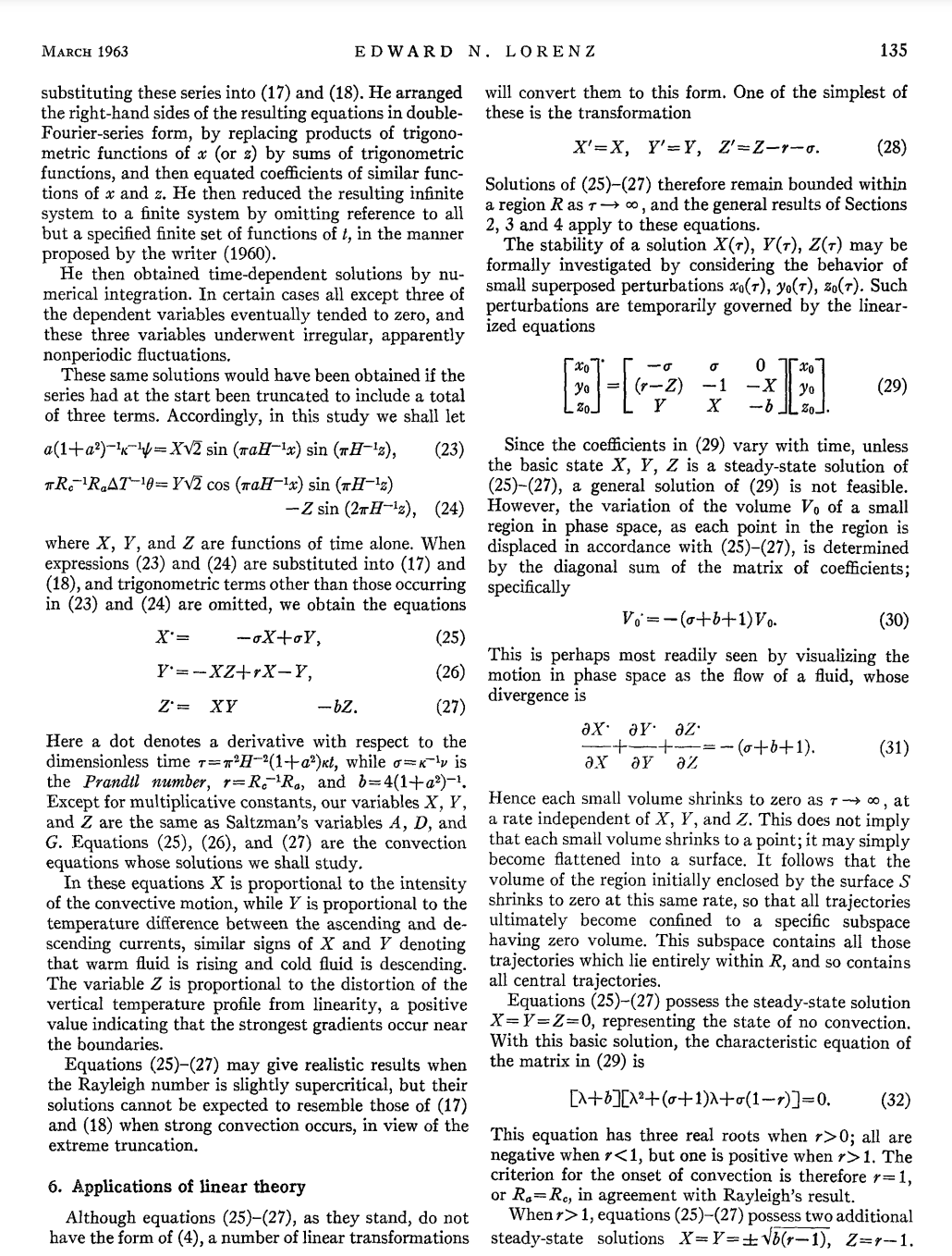
It was introduced in the 1960s

by Edward Norton Lorenz

Lorenz system

Lorenz E. N. (1963). Deterministic Nonperiodic Flow. Journal of the Atmospheric Sciences. 20(2): 130–141.

as a simplified mathematical model

for the atmospheric convection.

It was introduced in the 1960s

by Edward Norton Lorenz

Lorenz system

\displaystyle\left\{ \begin{array}{r} x(t,x,y,z)\\ \\ y(t,x,y,z)\\ \\ z(t,x,y,z) \end{array} \right.

We are looking for the functions

such that

\displaystyle\left\{ \begin{array}{rcl} x'&=&\sigma (-x + y)\\ \\ y'&=& -x z + \rho x - y \\ \\ z'&=& x y - \beta z \end{array} \right.

What does it mean to solve a system?

Lorenz system

\((x,y,z)\)

\(x\)

\(y\)

\(z\)

\displaystyle\left\{ \begin{array}{rcl} x'&=&\sigma (-x + y)\\ \\ y'&=& -x z + \rho x - y \\ \\ z'&=& x y - \beta z \end{array} \right.

The solution gives you the position

If the system represents the velocity of this particle

time

\(t\)

Lorenz system

\((x,y,z)\)

\(x\)

\(y\)

\(z\)

time

\(t\)

\displaystyle\left\{ \begin{array}{rcl} x'&=&\sigma (-x + y)\\ \\ y'&=& -x z + \rho x - y \\ \\ z'&=& x y - \beta z \end{array} \right.

The solution gives you the position

at any time \(t\)

General systems

\displaystyle\left\{ \begin{array}{rcl} x'_1&=&f_1(t,x_1,x_2,\ldots,x_n)\\ x'_2&=&f_2(t,x_1,x_2,\ldots,x_n)\\ x'_3&=&f_3(t,x_1,x_2,\ldots,x_n)\\ &\vdots& \\ x'_n&=&f_n(t,x_1,x_2,\ldots,x_n) \end{array} \right.

In general, solving systems of ODEs is incredibly difficult,

 sometimes even impossible!

The good news are that we still can solve them numerically!

General systems

\displaystyle\left\{ \begin{array}{rcl} x'_1&=&f_1(t,x_1,x_2,\ldots,x_n)\\ x'_2&=&f_2(t,x_1,x_2,\ldots,x_n)\\ x'_3&=&f_3(t,x_1,x_2,\ldots,x_n)\\ &\vdots& \\ x'_n&=&f_n(t,x_1,x_2,\ldots,x_n) \end{array} \right.

General systems

In GeoGebra we can use the command

 NSolveODE()

Here is where computers are quite useful

\displaystyle\left\{ \begin{array}{rcl} x'_1&=&f_1(t,x_1,x_2,\ldots,x_n)\\ x'_2&=&f_2(t,x_1,x_2,\ldots,x_n)\\ x'_3&=&f_3(t,x_1,x_2,\ldots,x_n)\\ &\vdots& \\ x'_n&=&f_n(t,x_1,x_2,\ldots,x_n) \end{array} \right.
NSolveODE(
	List of Derivatives, 
 	Initial x-coordinate, 
 	List of Initial y-coordinates, 
 	Final x-coordinate
)

Command

 NSolveODE()
\displaystyle\left\{ \begin{array}{rcl} x'&=&\sigma (-x + y)\\ \\ y'&=& -x z + \rho x - y \\ \\ z'&=& x y - \beta z \end{array} \right.

Initial time

\(t_0\)

Initial conditions

\((x_0,y_0,z_0)\) at \(t=t_0\)

Final time

\(t_f\)

Lorenz system

\((x_0,y_0,z_0)\)

\(x\)

\(y\)

\(z\)

time

\(t\)

\displaystyle\left\{ \begin{array}{rcl} x'&=&\sigma (-x + y)\\ \\ y'&=& -x z + \rho x - y \\ \\ z'&=& x y - \beta z \end{array} \right.

\(t_0\)

\(t_f\)

Lorenz system

\(x\)

\(y\)

\(z\)

time

\(t\)

\displaystyle\left\{ \begin{array}{rcl} x'&=&\sigma (-x + y)\\ \\ y'&=& -x z + \rho x - y \\ \\ z'&=& x y - \beta z \end{array} \right.

\(t_0\)

\(t_f\)

\((x_f,y_f,z_f)\)

\((x_0,y_0,z_0)\)

Chaotic behaviour

\displaystyle\left\{ \begin{array}{rcl} x'&=&\sigma (-x + y)\\ \\ y'&=& -x z + \rho x - y \\ \\ z'&=& x y - \beta z \end{array} \right.
(u_0,v_0,w_0)=(1,1.01,1)
(x_0,y_0,z_0)=(1,1,1)
d = 10
b = 8/3
p = 28

x'(t,x,y,z) = d * (y - x)
y'(t,x,y,z) = x * (p - z) - y
z'(t,x,y,z) = x * y - b * z

x0 = 1
y0 = 1
z0 = 1

NSolveODE({x', y', z'}, 0, {x0, y0, z0}, 20)

len = Length(numericalIntegral1)

L_1 = Sequence( (y(Point(numericalIntegral1, i)), y(Point(numericalIntegral2, i)), y(Point(numericalIntegral3, i))), i, 0, 1, 1 / len )

f = Polyline(L_1)

Script

The algorithm behind this command is based on

Runge-Kutta numeric methods

Command

 NSolveODE()
NSolveODE(
	List of Derivatives, 
 	Initial x-coordinate, 
 	List of Initial y-coordinates, 
 	Final x-coordinate
)