Recent advances in trustworthy machine learning for computational imaging

Jeremias Sulam

AWS Responsible AI Seminar

"The biggest lesson that can be read from 70 years of AI research is that general methods that leverage computation are ultimately the most effective, and by a large margin. [...] Seeking an improvement that makes a difference in the shorter term, researchers seek to leverage their human knowledge of the domain, but the only thing that matters in the long run is the leveraging of computation. [...]
We want AI agents that can discover like we can, not which contain what we have discovered."

The Bitter Lesson, Rich Sutton 2019

{f}\huge(

{\huge)} = \text{\texttt{sick}}

What parts of the image are important for this prediction?

What are the subsets of the input so that

{f}(x_C) \approx {f}(x) ?

C \subseteq [d]

Interpretability in Image Classification

Sensitivity or Gradient-based perturbations
Shapley coefficients
Variational formulations
Counterfactual & causal explanations

LIME [Ribeiro et al, '16], CAM [Zhou et al, '16], Grad-CAM [Selvaraju et al, '17]

Shap [Lundberg & Lee, '17], ...

RDE [Macdonald et al, '19], ...

[Sani et al, 2020] [Singla et al '19],..

Post-hoc Interpretability in Image Classification

Sensitivity or Gradient-based perturbations
Shapley coefficients
Variational formulations
Counterfactual & causal explanations

LIME [Ribeiro et al, '16], CAM [Zhou et al, '16], Grad-CAM [Selvaraju et al, '17]

Shap [Lundberg & Lee, '17], ...

RDE [Macdonald et al, '19], ...

[Sani et al, 2020] [Singla et al '19],..

Post-hoc Interpretability in Image Classification

Adebayo et al, Sanity checks for saliency maps, 2018
Ghorbani et al, Interpretation of neural networks is fragile, 2019
Shah et al, Do input gradients highlight discriminative features? 2021

Sensitivity or Gradient-based perturbations
Shapley coefficients
Variational formulations
Counterfactual & causal explanations

LIME [Ribeiro et al, '16], CAM [Zhou et al, '16], Grad-CAM [Selvaraju et al, '17]

Shap [Lundberg & Lee, '17], ...

RDE [Macdonald et al, '19], ...

[Sani et al, 2020] [Singla et al '19],..

Post-hoc Interpretability in Image Classification

Post-hoc Interpretability Methods

Interpretable by

construction

Adebayo et al, Sanity checks for saliency maps, 2018
Ghorbani et al, Interpretation of neural networks is fragile, 2019
Shah et al, Do input gradients highlight discriminative features? 2021

Sensitivity or Gradient-based perturbations
Shapley coefficients
Variational formulations
Counterfactual & causal explanations

LIME [Ribeiro et al, '16], CAM [Zhou et al, '16], Grad-CAM [Selvaraju et al, '17]

Shap [Lundberg & Lee, '17], ...

RDE [Macdonald et al, '19], ...

[Sani et al, 2020] [Singla et al '19],..

Post-hoc Interpretability in Image Classification

Post-hoc Interpretability Methods

Interpretable by

construction

Adebayo et al, Sanity checks for saliency maps, 2018
Ghorbani et al, Interpretation of neural networks is fragile, 2019
Shah et al, Do input gradients highlight discriminative features? 2021

efficiency
nullity
symmetry

exponential complexity

Lloyd S Shapley. A value for n-person games. Contributions to the Theory of Games, 2(28):307–317, 1953.

Let be an -person cooperative game with characteristic function

G = ([n],f)

f : \mathcal P([n]) \mapsto \mathbb R

How important is each player for the outcome of the game?

\displaystyle \phi_i = \sum_{S_j\subseteq [n]\setminus \{i\} } w_{S_j} \left[ f(S_j\cup \{i\}) - f(S_j) \right]

marginal contribution of player i with coalition S

Shapley values

f \approx \mathbb E[Y|X=x]

X \in \mathcal X \subset \mathbb R^n

Y\in \mathcal Y = \{0,1\}

inputs

responses

f:\mathcal X \to \mathcal Y

\text{For any}~ S \subset [n],~ \text{and a sample } { x} \newline \text{ define }\tilde{X}_S = [{x_S},X_{S^c}], \text{ where } X_{S^c}\sim \mathcal D_{X_S={x_S}}

predictor

Shap-Explanations

x_S

x_{S^c}

f \approx \mathbb E[Y|X=x]

X \in \mathcal X \subset \mathbb R^n

Y\in \mathcal Y = \{0,1\}

inputs

responses

f:\mathcal X \to \mathcal Y

\text{For any}~ S \subset [n],~ \text{and a sample } { x} \newline \text{ define }\tilde{X}_S = [{x_S},X_{S^c}], \text{ where } X_{S^c}\sim \mathcal D_{X_S={x_S}}

predictor

Shap-Explanations

x_S

x_{S^c}

\tilde{X}_S:

Shap-Explanations

x_S

\tilde{X}_S

f \approx \mathbb E[Y|X=x]

X \in \mathcal X \subset \mathbb R^n

Y\in \mathcal Y = \{0,1\}

inputs

responses

f:\mathcal X \to \mathcal Y

\text{For any}~ S \subset [n],~ \text{and a sample } { x} \newline \text{ define }\tilde{X}_S = [{x_S},X_{S^c}], \text{ where } X_{S^c}\sim \mathcal D_{X_S={x_S}}

predictor

\displaystyle \phi_i = \sum_{S_j\subseteq [n]\setminus \{i\}} w_j ~ \mathbb E \left[ f(\tilde X_{S_j\cup \{i\}}) - f(\tilde X_{S_j}) \right]

Scott Lundberg and Su-In Lee. A Unified Approach to Interpreting Model Predictions, NeurIPS , 2017

Shap-Explanations

f \approx \mathbb E[Y|X=x]

X \in \mathcal X \subset \mathbb R^n

Y\in \mathcal Y = \{0,1\}

inputs

responses

f:\mathcal X \to \mathcal Y

\text{For any}~ S \subset [n],~ \text{and a sample } { x} \newline \text{ define }\tilde{X}_S = [{x_S},X_{S^c}], \text{ where } X_{S^c}\sim \mathcal D_{X_S={x_S}}

predictor

Guiding Questions

Question 1)

Can we resolve the computational bottleneck (and when)?

Question 2)

What do these coefficients mean, statistically?

Question 3)

How to go beyond input-features explanations?

Time permitting... an observation on fairness

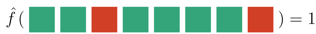
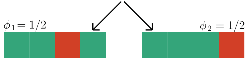
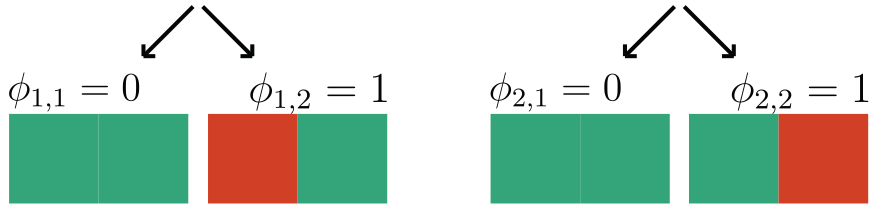
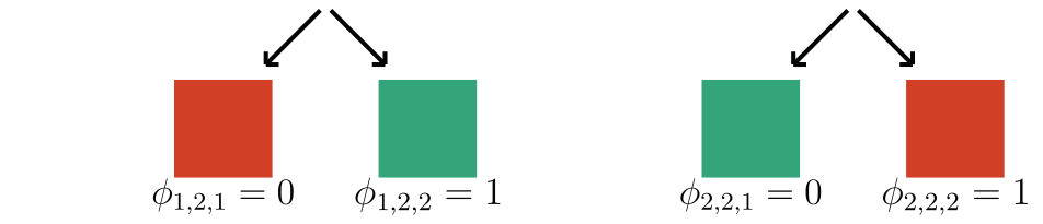
We focus on data with certain structure:

f\huge(

{\huge)} = 0

{f}\huge(

{\huge)} = 1

{f}\huge(

{\huge)} = 0

Example:

f(x) = 1

if contains a sick cell

Hierarchical Shap (h-Shap)

\text{\textbf{Assumption 1:}}~ f(x) = 1 \Leftrightarrow \exist~ i: f(\tilde X_i) = 1

Question 1) Can we resolve the computational bottleneck (and when) ?

\gamma = 2

We focus on data with certain structure:

\text{\textbf{Assumption 1:}}~ f(x) = 1 \Leftrightarrow \exist~ i: f(\tilde X_i) = 1

Theorem (informal)

h-Shap runs in linear time
Under A1, h-Shap \(\to\) Shapley

\mathcal O(2^\gamma k \log n)

Hierarchical Shap (h-Shap)

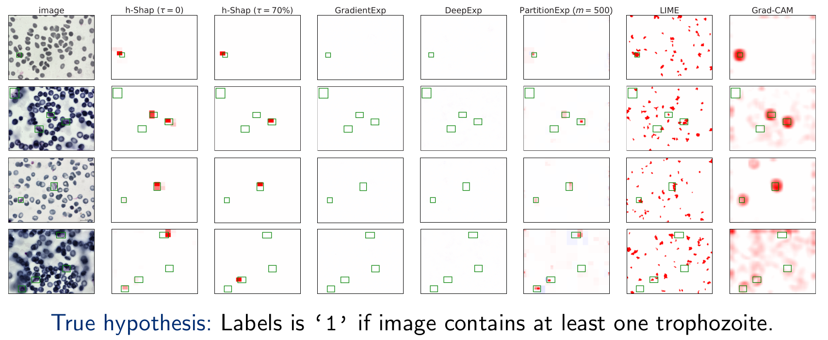
Hierarchical Shap (h-Shap)

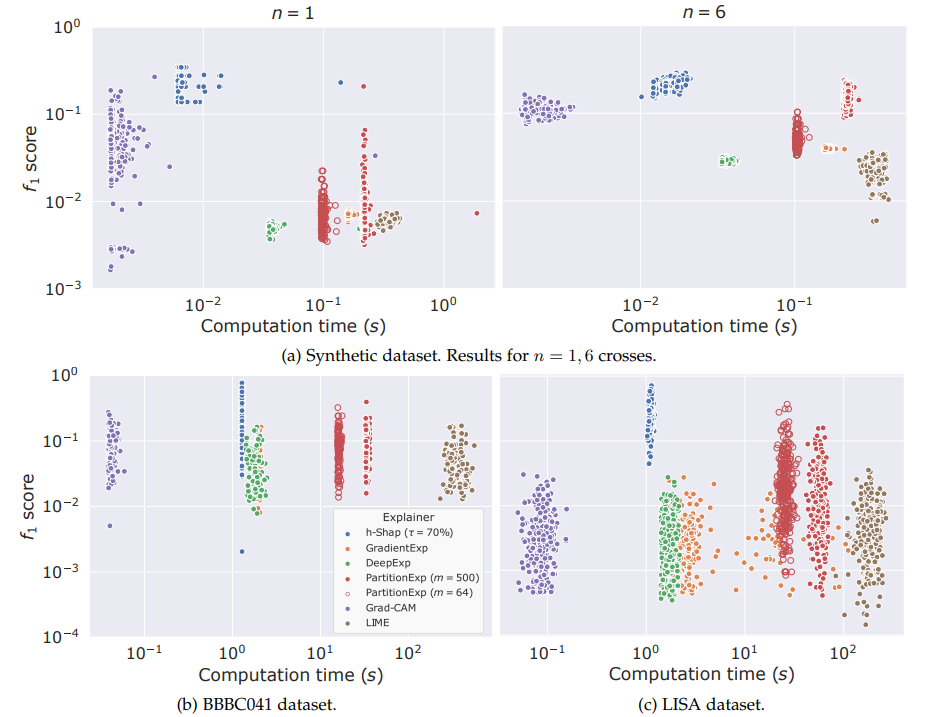
Fast hierarchical games for image explanations, Teneggi, Luster & S., IEEE Transactions on Pattern Analysis and Machine Intelligence, 2022

Hierarchical Shap (h-Shap)

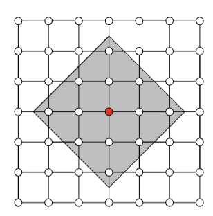
Other notions of structure

Local models

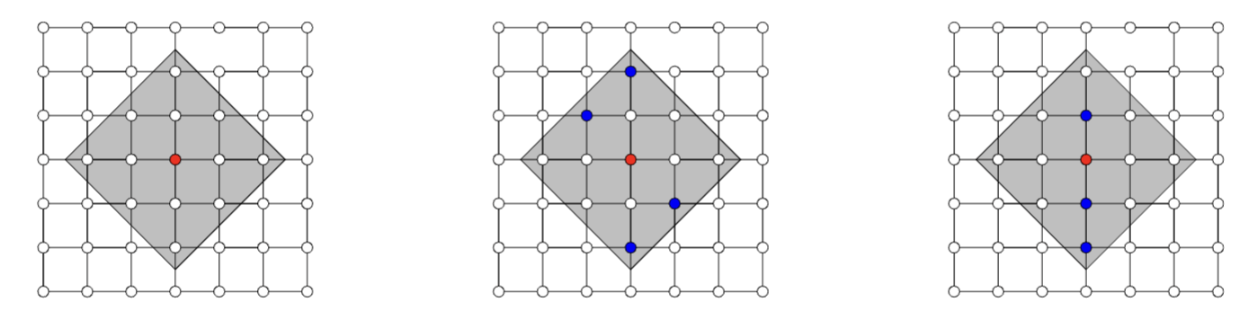
Observation: Restrict computation of \(\phi_i(f)\) to local areas of influence given by a graph structure

L-Shap

C-Shap

\displaystyle \hat{\phi}^k_i(v) = \frac{1}{|\mathcal N_k(i)|} \sum_{S\subseteq\mathcal N_k(i)\setminus i } w(S) \left[ v(S\cup \{i\}) - v(S) \right]

\(\Rightarrow\) complexity \(\mathcal O(2^k n)\)

[Chen et al, 2019]

Other notions of structure

Local models

[Chen et al, 2019]

Observation: Restrict computation of \(\phi_i(f)\) to local areas of influence given by a graph structure

\(\Rightarrow\) complexity \(\mathcal O(2^k n)\)

Correct approximations (informal statement)

Let \(S\subset \mathcal N_k(i)\). If \((X_i \perp\!\!\!\perp X_{[n]\setminus S} | X_T) \) and \((X_i \perp\!\!\!\perp X_{[n]\setminus S} | X_T,Y) \) for any \(T\subset S\setminus i\).

Then \(\hat{\phi}^k_i(v) = \phi_i(v)\)

(and approximately bounded otherwise, controlled)

\displaystyle \hat{\phi}^k_i(v) = \frac{1}{|\mathcal N_k(i)|} \sum_{S\subseteq\mathcal N_k(i)\setminus i } w(S) \left[ v(S\cup \{i\}) - v(S) \right]

Question 2) What do these coefficients mean, statistically?

Precise notions of importance

Formal Feature Importance

H_{0,S}:~ X_S \perp\!\!\!\perp Y | X_{[n]\setminus S}

[Candes et al, 2018]

Question 2) What do these coefficients mean, statistically?

Precise notions of importance

XRT: eXplanation Randomization Test

returns a \(\hat{p}_{i,S}\) for the test above

\text{reject} ~\Rightarrow~ i=2 \text{: important}

H^0_{i=2,S=\{1,3,4\}}

i=1

i=2

i=3

i=4

How do we test?

\text{For any } S \subseteq [n]\setminus \{{\color{Red}i}\}, \text{ and a sample } x\sim \mathcal p_X

H^0_{{\color{red}i},S}:~ (f(\tilde X_{S\cup \{{\color{red}i}\}}) ) \overset{d}{=} (f(\tilde X_{S}) )

Local Feature Importance

Precise notions of importance

Local Feature Importance

\text{For any } S \subseteq [n]\setminus \{{\color{Red}i}\}, \text{ and a sample } x\sim \mathcal D_X

H^0_{{\color{red}i},S}:~ (f(\tilde X_{S\cup \{{\color{red}i}\}}) ) \overset{d}{=} (f(\tilde X_{S}) )

\gamma_{i,S}

\displaystyle \phi_{\color{red}i}(x) = \sum_{S\subseteq [n]\setminus \{{\color{red}i}\}} w_{S} ~ \mathbb E \left[ f(\tilde X_{S\cup \{{\color{red}i}\}}) - f(\tilde X_S) \right]

Given the Shapley coefficient of any feature

Then

p_{i,S}

and the (expected) p-value obtained for , i.e. ,

H^0_{i,S}

Theorem:

p_{i,S} \leq 1 - \gamma_{i,S}.

i\in[n],

Teneggi, Bharti, Romano, and S. "SHAP-XRT: The Shapley Value Meets Conditional Independence Testing." TMLR (2023).

Question 3)

How to go beyond input-features explanations?

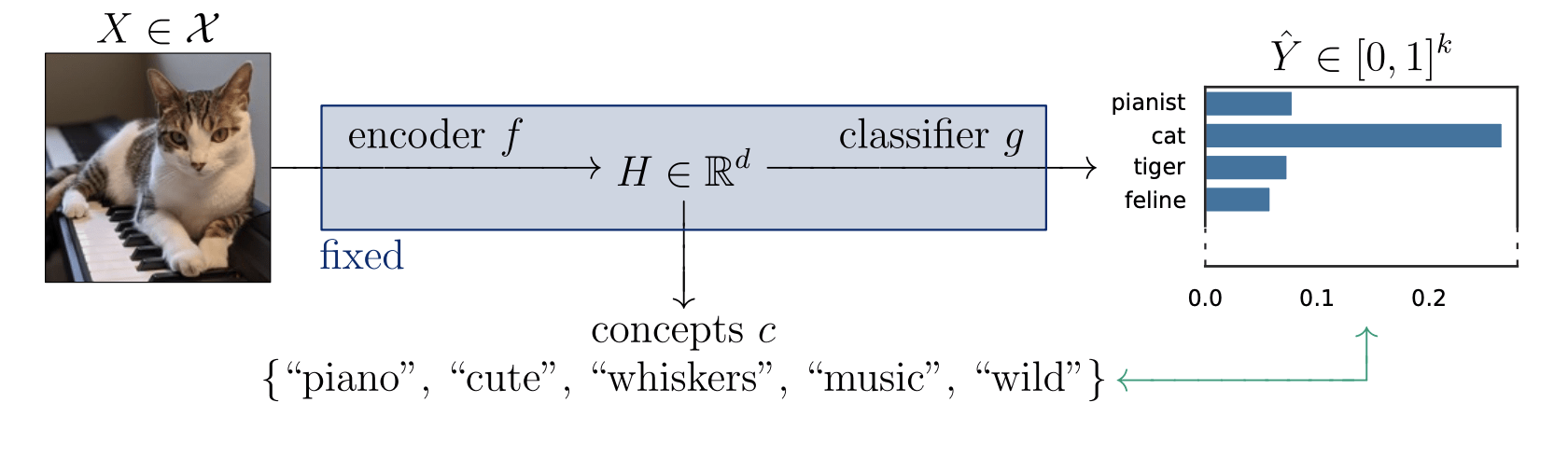
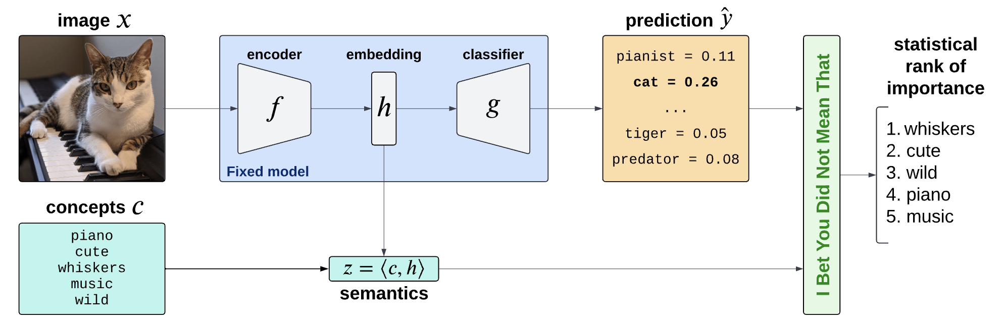
Is the piano important for \(\hat Y = \text{cat}\)?

How can we explain black-box predictors with semantic features?

Is the piano important for \(\hat Y = \text{cat}\), given that there is a cute mammal in the image?

Semantic Interpretability of classifiers

Is the presence of \(\color{Blue}\texttt{edema}\) important for \(\hat Y = \text{lung opacity}\)?

How can we explain black-box predictors with semantic features?

Is the presence of \(\color{magenta}\texttt{devices}\) important for \(\hat Y = \texttt{lung opacity}\), given that there is \(\color{blue}\texttt{edema}\) in the image?

model-agnostic interpretability

lung opacity

cardiomegaly

fracture

no findding

Semantic Interpretability of classifiers

Concept Bank: \(C = [c_1, c_2, \dots, c_m] \in \mathbb R^{d\times m}\)

Embeddings: \(H = f(X) \in \mathbb R^d\)

Semantics: \(Z = C^\top H \in \mathbb R^m\)

Concept Bank: \(C = [c_1, c_2, \dots, c_m] \in \mathbb R^{d\times m}\)

Concept Activation Vectors

(Kim et al, 2018)

\(c_\text{cute}\)

Semantic Interpretability of classifiers

Vision-language models

(CLIP, BLIP, etc... )

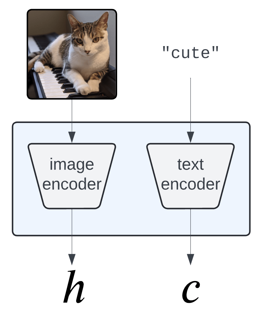
Semantic Interpretability of classifiers

Concept Bank: \(C = [c_1, c_2, \dots, c_m] \in \mathbb R^{d\times m}\)

Vision-language models

(training)

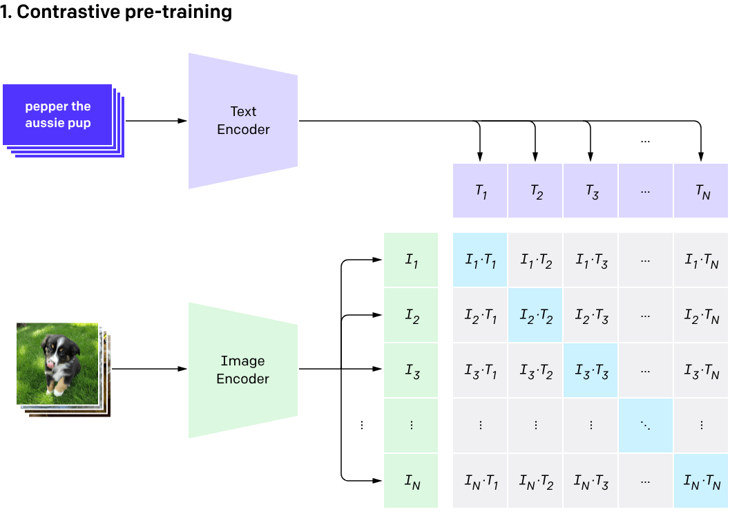
[Radford et al, 2021]

Semantic Interpretability of classifiers

[Bhalla et al, "Splice", 2024]

Concept Bottleneck Models (CMBs)

[Koh et al '20, Yang et al '23, Yuan et al '22 ]

Need to engineer a (large) concept bank
Performance hit w.r.t. original predictor

\(\tilde{Y} = \hat w^\top Z\)

\(\hat w_j\) is the importance of the \(j^{th}\) concept

Desiderata

Fixed original predictor (post-hoc)
Global and local importance notions
Testing for any concepts (no need for large concept banks)
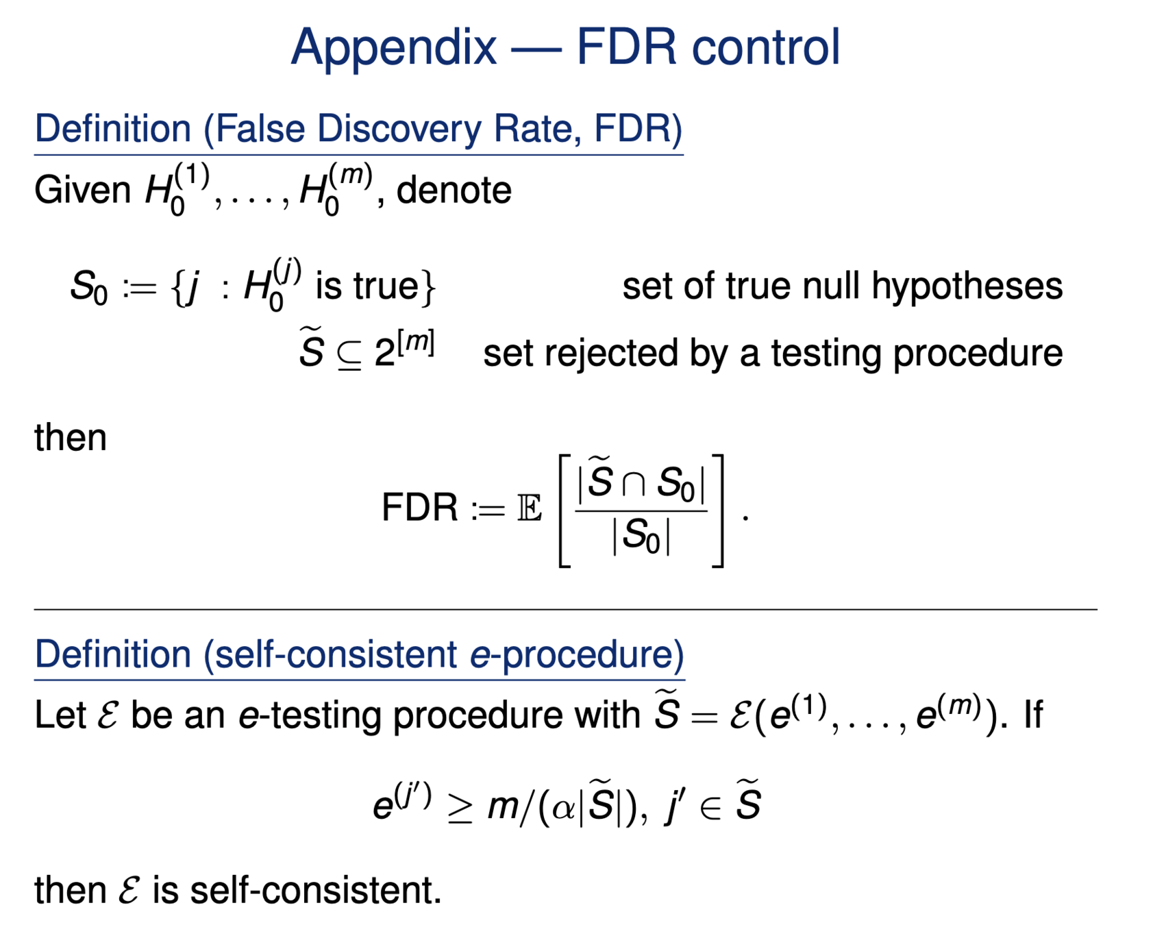
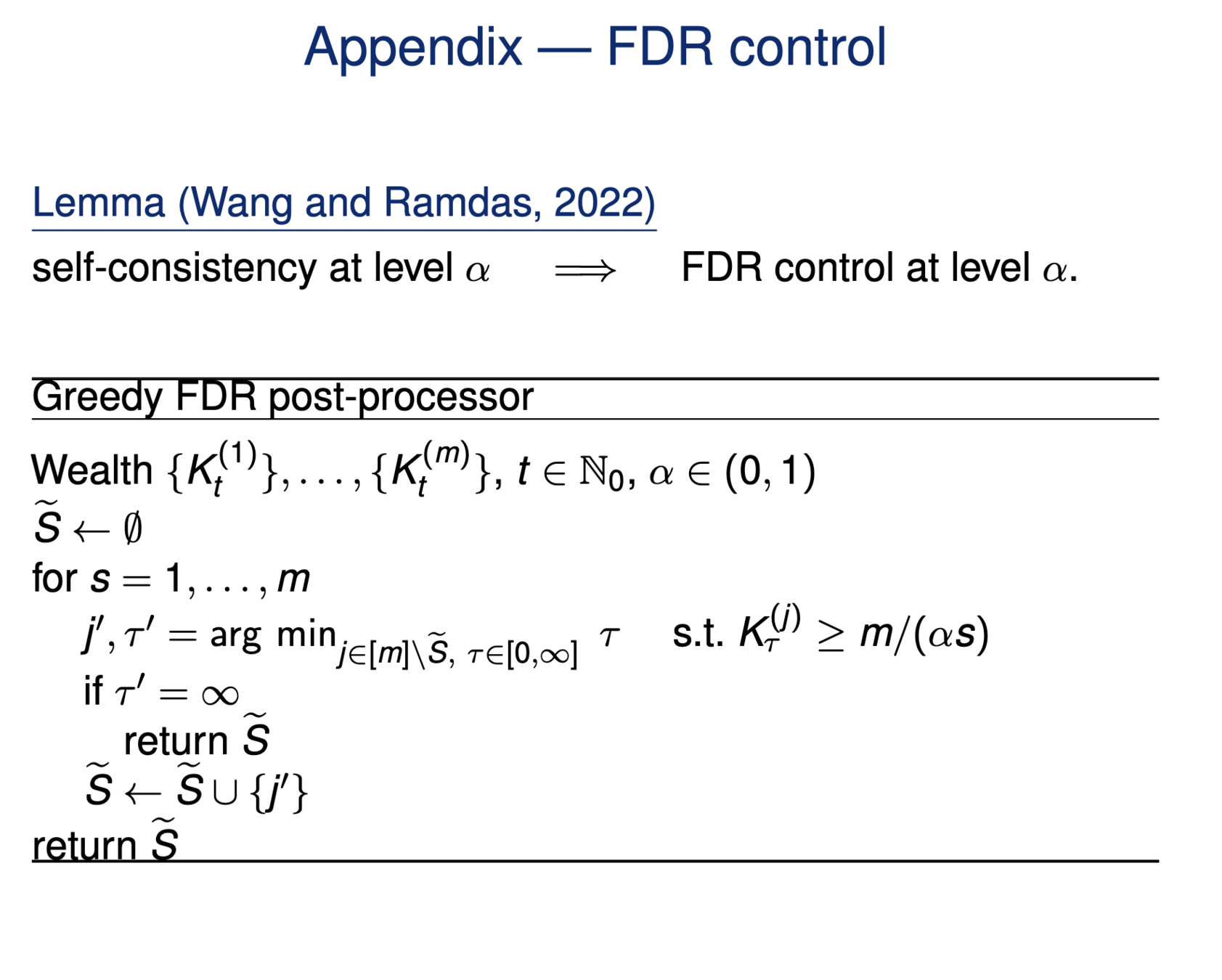
Precise testing with guarantees (Type 1 error/FDR control)

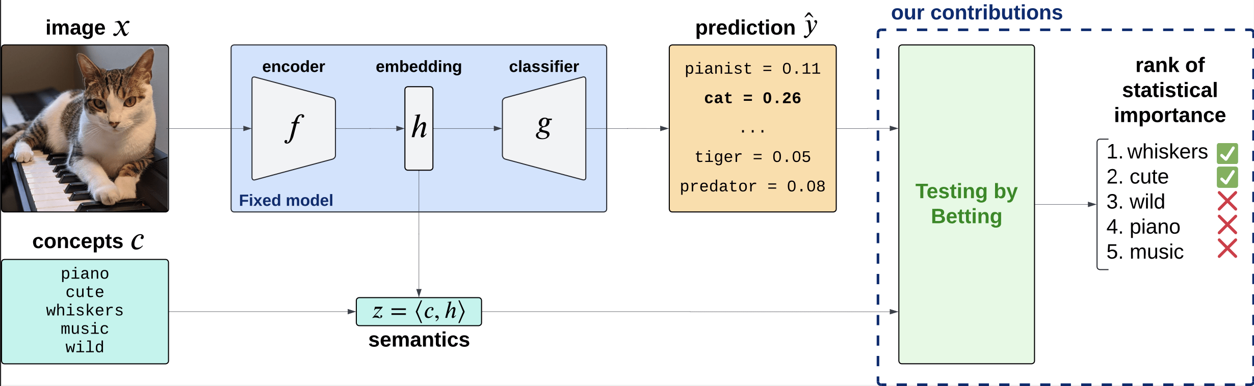
Precise notions of semantic importance

\(C = \{\text{``cute''}, \text{``whiskers''}, \dots \}\)

Global Importance

\(H^G_{0,j} : \hat{Y} \perp\!\!\!\perp Z_j \)

Global Conditional Importance

\(H^{GC}_{0,j} : \hat{Y} \perp\!\!\!\perp Z_j | Z_{-j}\)

Precise notions of semantic importance

Global Importance

\(C = \{\text{``cute''}, \text{``whiskers''}, \dots \}\)

\(H^G_{0,j} : g(f(X)) \perp\!\!\!\perp c_j^\top f(X) \)

Global Conditional Importance

\(H^{GC}_{0,j} : g(f(X)) \perp\!\!\!\perp c_j^\top f(X) | C_{-j}^\top f(X)\)

\(H^G_{0,j} : \hat{Y} \perp\!\!\!\perp Z_j \)

\(H^{GC}_{0,j} : \hat{Y} \perp\!\!\!\perp Z_j | Z_{-j}\)

Precise notions of semantic importance

"The classifier (its distribution) does not change if we condition

on concepts \(S\) vs on concepts \(S\cup\{j\} \)"

\(C = \{\text{``cute''}, \text{``whiskers''}, \dots \}\)

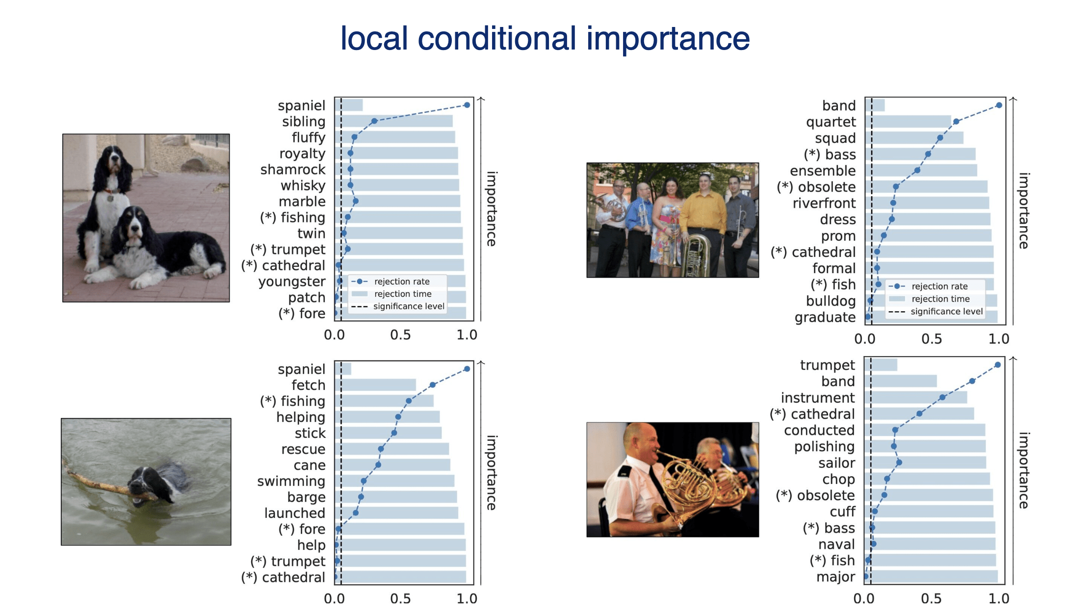
Local Conditional Importance

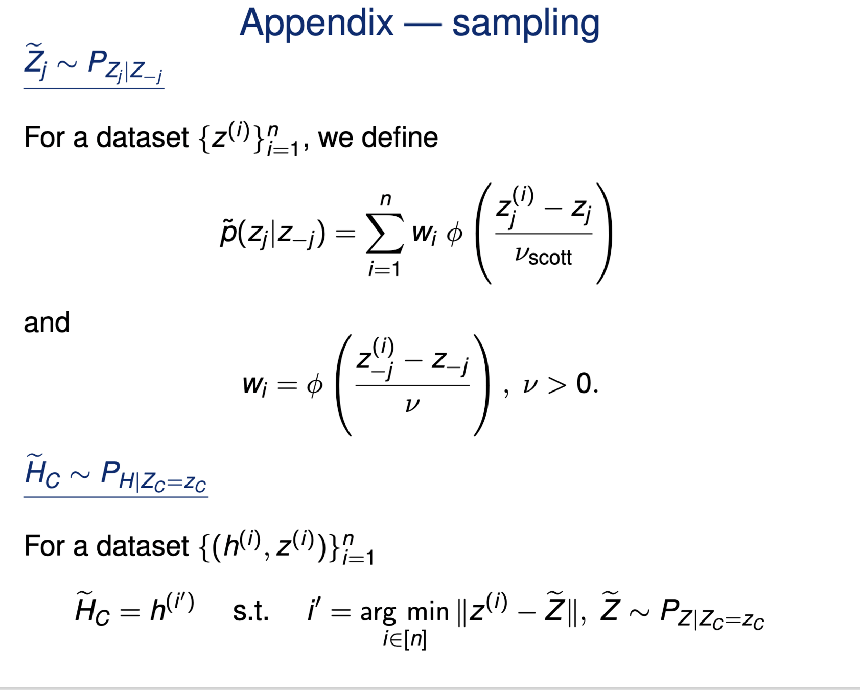
\[H^{j,S}_0:~ g({\tilde H_{S \cup \{j\}}}) \overset{d}{=} g(\tilde H_S), \qquad \tilde H_S \sim P_{H|Z_S = C_S^\top f(x)} \]

Precise notions of semantic importance

"The classifier (its distribution) does not change if we condition

on concepts \(S\) vs on concepts \(S\cup\{j\} \)"

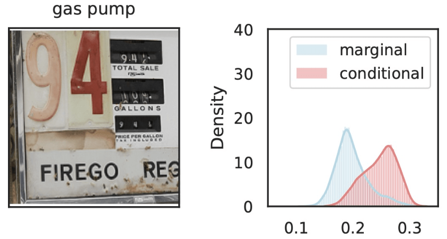
\(\hat{Y}_\text{gas pump}\)

\(Z_S\cup Z_{j}\)

\(Z_{S}\)

\(Z_j=\)

Local Conditional Importance

\[H^{j,S}_0:~ g({\tilde H_{S \cup \{j\}}}) \overset{d}{=} g(\tilde H_S), \qquad \tilde H_S \sim P_{H|Z_S = C_S^\top f(x)} \]

Precise notions of semantic importance

"The classifier (its distribution) does not change if we condition

on concepts \(S\) vs on concepts \(S\cup\{j\} \)"

\(\hat{Y}_\text{gas pump}\)

\(Z_S\cup Z_{j}\)

\(Z_{S}\)

\(Z_S\cup Z_{j}\)

\(Z_{S}\)

Local Conditional Importance

\(Z_j=\)

\[H^{j,S}_0:~ g({\tilde H_{S \cup \{j\}}}) \overset{d}{=} g(\tilde H_S), \qquad \tilde H_S \sim P_{H|Z_S = C_S^\top f(x)} \]

we can sample from these

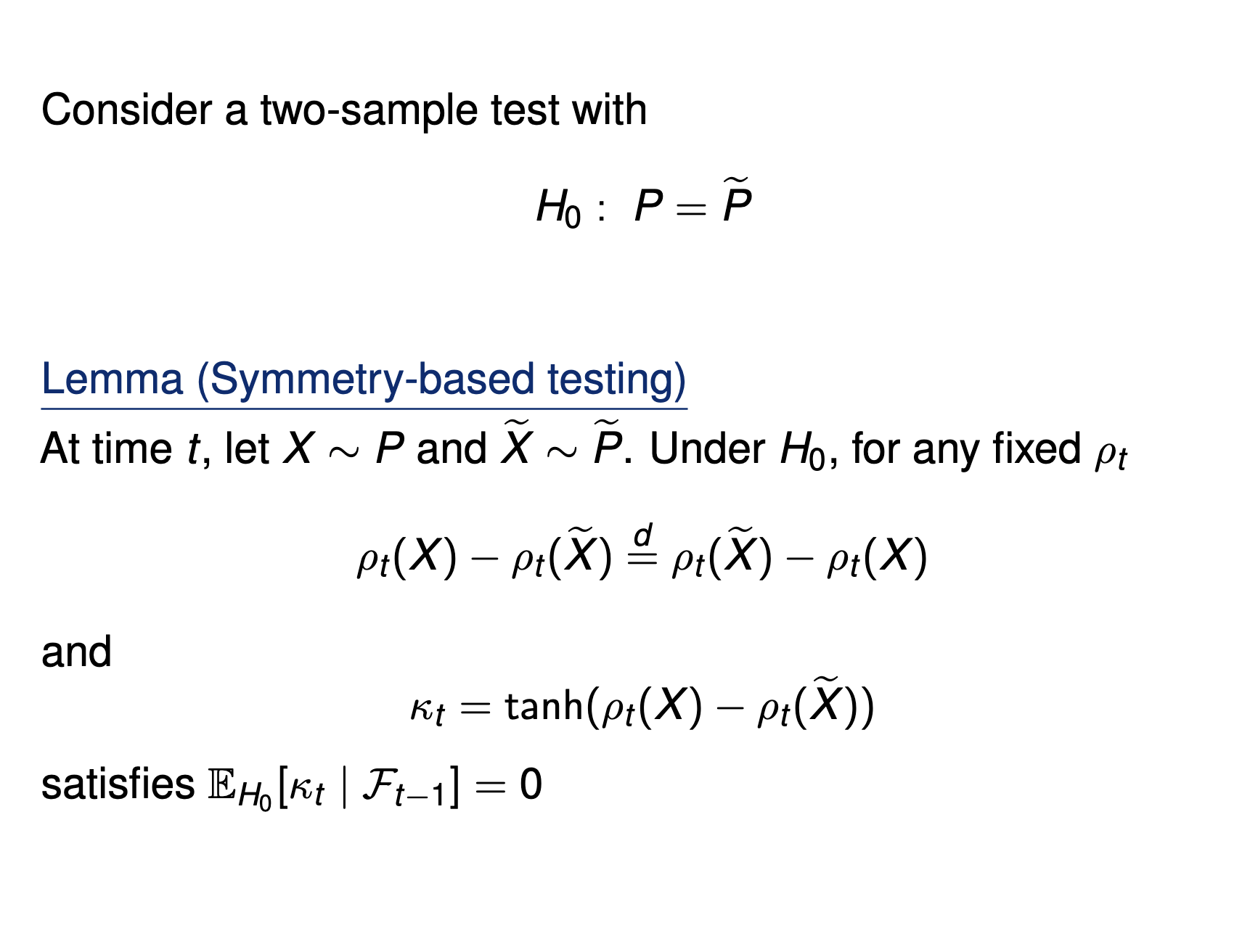
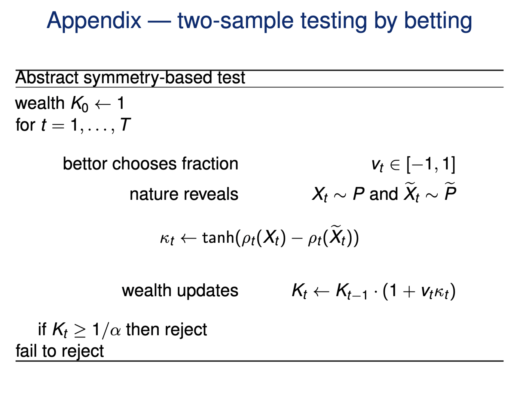
Testing by betting

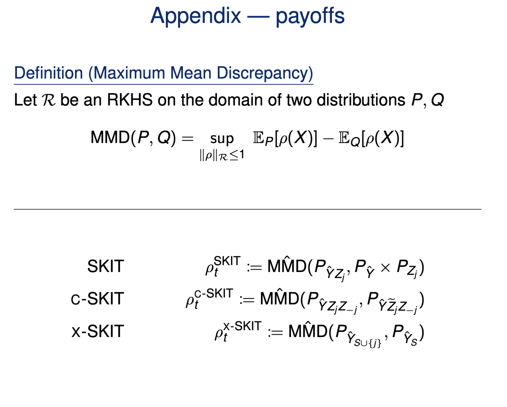
\(H^G_{0,j} : \hat{Y} \perp\!\!\!\perp Z_j \iff P_{\hat{Y},Z_j} = P_{\hat{Y}} \times P_{Z_j}\)

Testing importance via two-sample tests

\(H^{GC}_{0,j} : \hat{Y} \perp\!\!\!\perp Z_j | Z_{-j} \iff P_{\hat{Y}Z_jZ_{-j}} = P_{\hat{Y}\tilde{Z}_j{Z_{-j}}}\)

\(\tilde{Z_j} \sim P_{Z_j|Z_{-j}}\)

[Shaer et al, 2023]

[Teneggi et al, 2023]

\[H^{j,S}_0:~ g({\tilde H_{S \cup \{j\}}}) \overset{d}{=} g(\tilde H_S), \qquad \tilde H_S \sim P_{H|Z_S = C_S^\top f(x)} \]

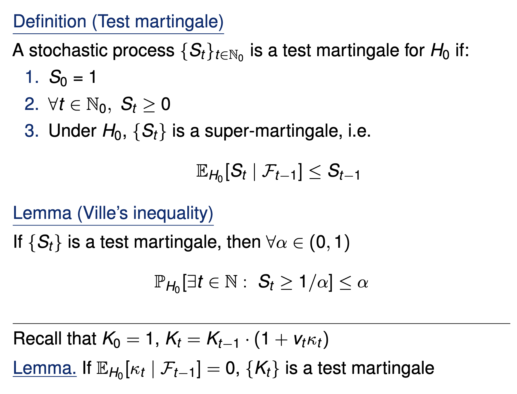
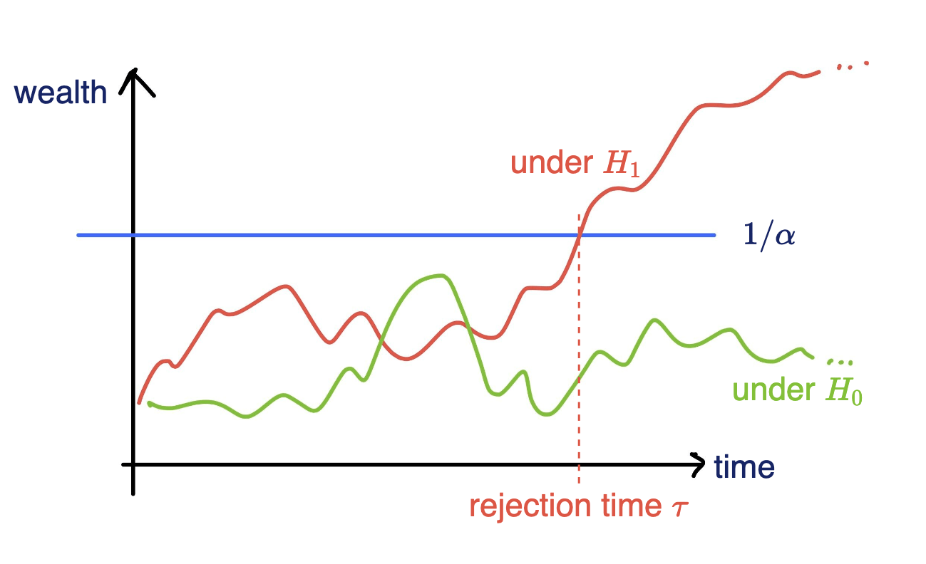
Testing by betting

Goal: Test a null hypothesis \(H_0\) at significance level \(\alpha\)

Standard testing by p-values

Collect data, then test, and reject if \(p \leq \alpha\)

Online testing by e-values

Any-time valid inference, monitor online and reject when \(e\geq 1/\alpha\)

[Shaer et al. 2023, Shekhar and Ramdas 2023, Podkopaev et al 2023]

Testing by betting via SKIT (Podkopaev et al., 2023)

Online testing by e-values

Any-time valid inference, track and reject when \(e\geq 1/\alpha\)

Consider a wealth process
\(K_0 = 1;\)
\(\text{for}~ t = 1, \dots \\ \quad K_t = K_{t-1}(1+\kappa_t v_t)\)

Fair game (test martingale): \(~~\mathbb E_{H_0}[\kappa_t | \text{Everything seen}_{t-1}] = 0\)

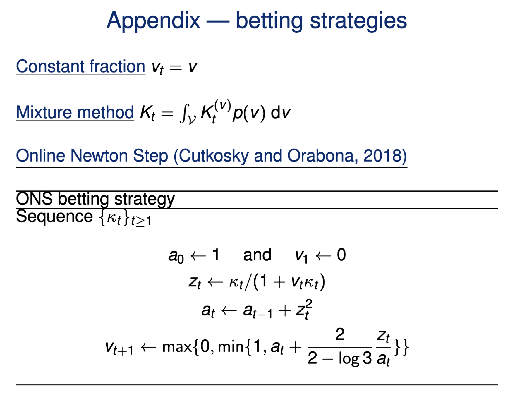
\(v_t \in (0,1):\) betting fraction

\(\kappa_t \in [-1,1]\) payoff

[Grünwald 2019, Shafer 2021, Shaer et al. 2023, Shekhar and Ramdas 2023. Podkopaev et al., 2023]

\(\mathbb P_{H_0}[\exists t \in \mathbb N: K_t \leq 1/\alpha]\leq \alpha\)

Goal: Test a null hypothesis \(H_0\) at significance level \(\alpha\)

Testing by betting via SKIT (Podkopaev et al., 2023)

Online testing by e-values

Any-time valid inference, track and reject when \(e\geq 1/\alpha\)

Consider a wealth process
\(K_0 = 1;\)
\(\text{for}~ t = 1, \dots \\ \quad K_t = K_{t-1}(1+\kappa_t v_t)\)

Fair game (test martingale): \(~~\mathbb E_{H_0}[\kappa_t | \text{Everything seen}_{t-1}] = 0\)

\(v_t \in (0,1):\) betting fraction

\(\kappa_t \in [-1,1]\) payoff

[Grünwald 2019, Shafer 2021, Shaer et al. 2023, Shekhar and Ramdas 2023. Podkopaev et al., 2023]

\(\mathbb P_{H_0}[\exists t \in \mathbb N: K_t \leq 1/\alpha]\leq \alpha\)

Goal: Test a null hypothesis \(H_0\) at significance level \(\alpha\)

Data efficient

Rank induced by rejection time

Online testing by e-values

\(v_t \in (0,1):\) betting fraction

\(H_0: ~ P = Q\)

\(\kappa_t = \text{tahn}({\color{teal}\rho(X_t)} - {\color{teal}\rho(Y_t)})\)

Payoff function

\({\color{black}\text{MMD}(P,Q)} : \text{ Maximum Mean Discrepancy}\)

\({\color{teal}\rho} = \underset{\rho\in \mathcal R:\|\rho\|_\mathcal R\leq 1}{\arg\sup} ~\mathbb E_P [\rho(X)] - \mathbb E_Q[\rho(Y)]\)

\( K_t = K_{t-1}(1+\kappa_t v_t)\)

Data efficient

Rank induced by rejection time

Testing by betting via SKIT (Podkopaev et al., 2023)

[Shaer et al. 2023, Shekhar and Ramdas 2023, Podkopaev et al 2023]

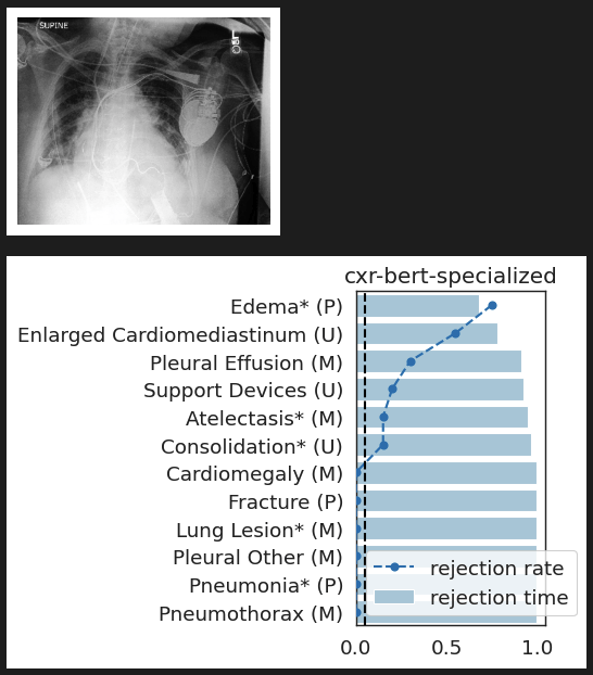
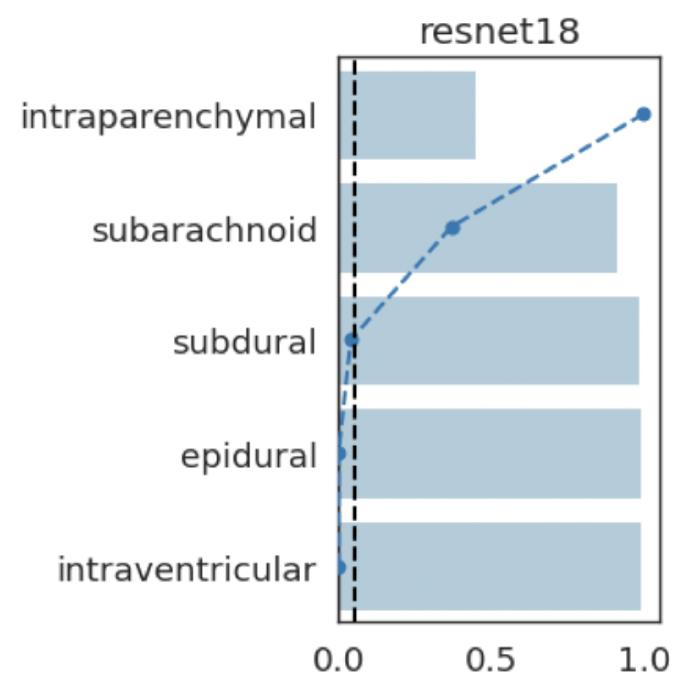
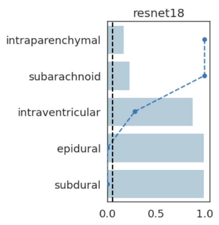
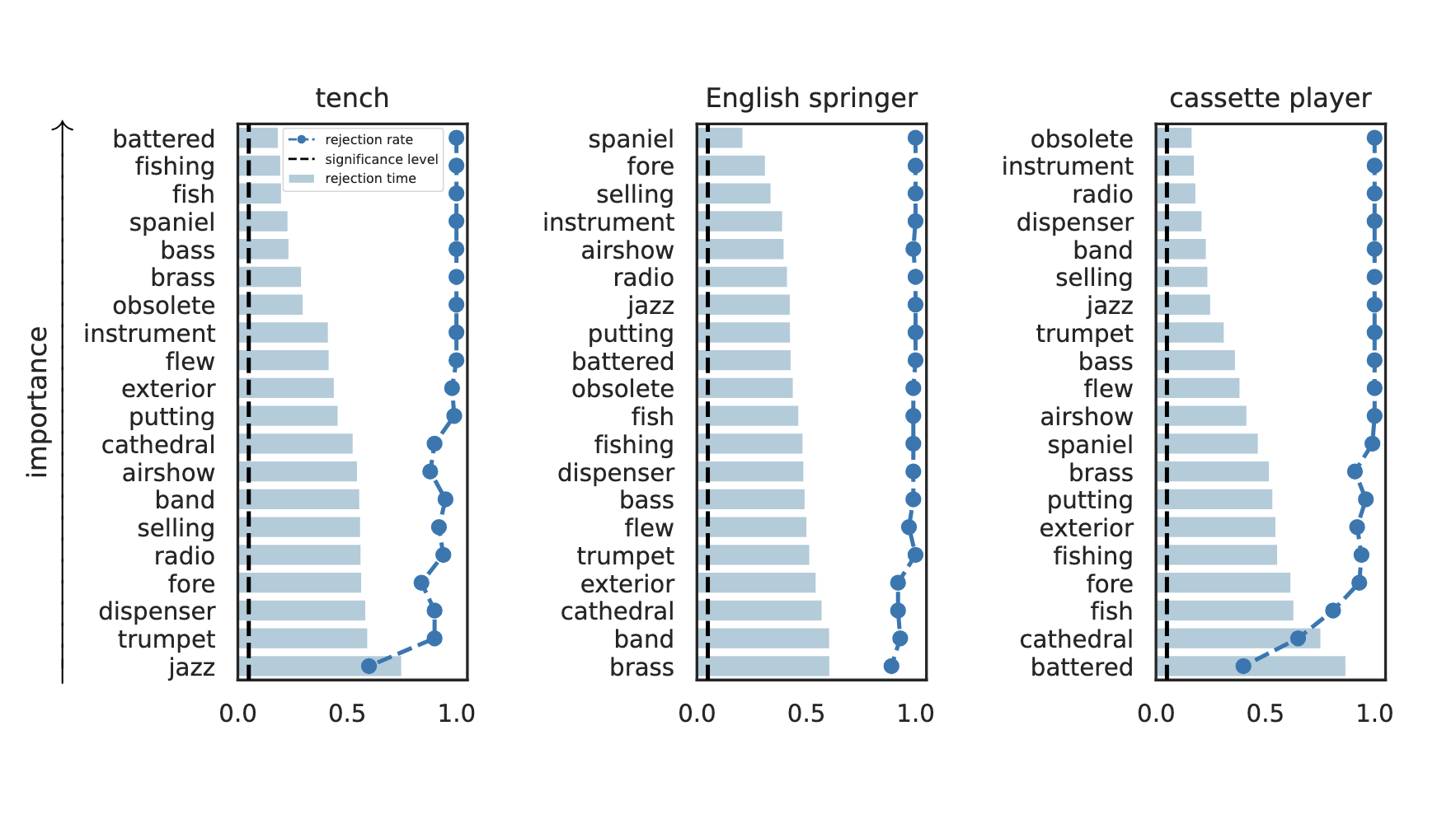
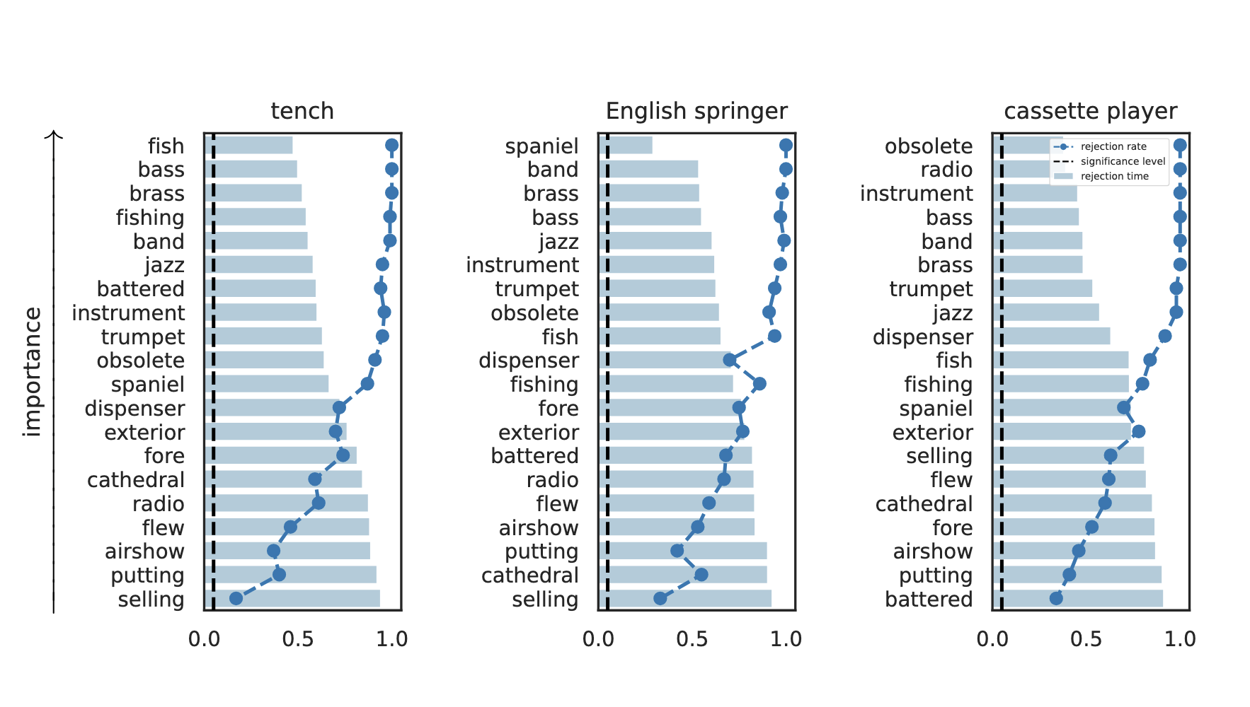
rejection time

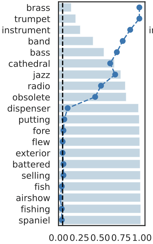
rejection rate

Important Semantic Concepts
(Reject \(H_0\))

Unimportant Semantic Concepts

(fail to reject \(H_0\))

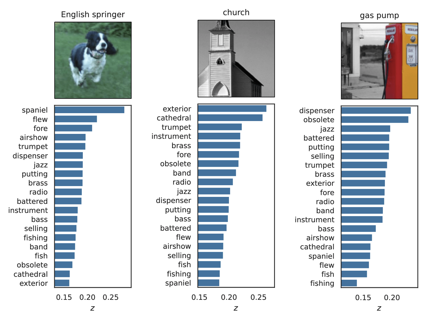
Results: Imagenette

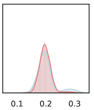
Type 1 error control

False discovery rate control

Results: Imagenette

Results: Imagenette

Results: CUB dataset

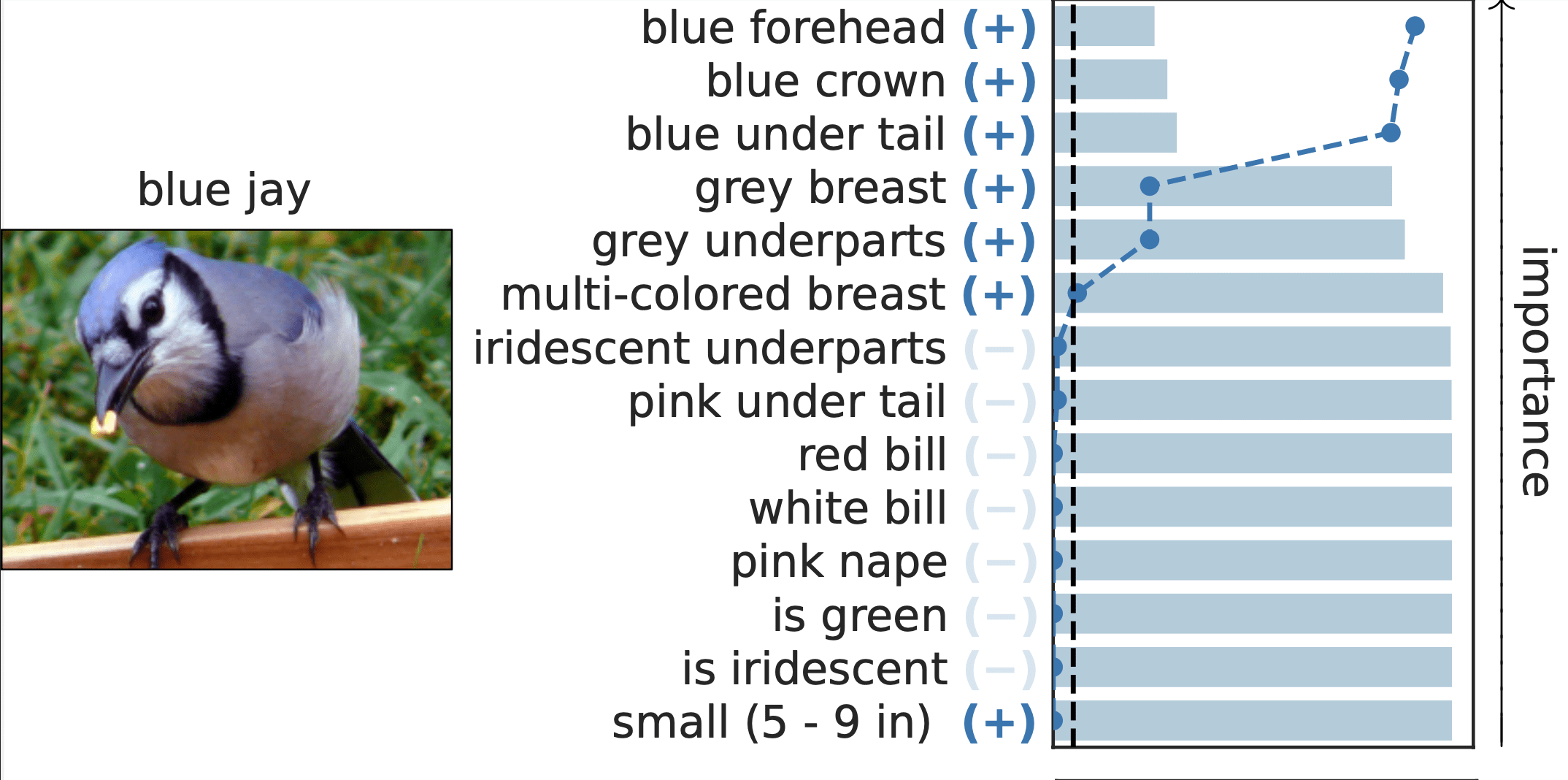
Important Semantic Concepts
(Reject \(H_0\))

Unimportant Semantic Concepts

(Fail to reject)

rejection time

rejection rate

0.0

1.0

CheXpert: validating BiomedVLP

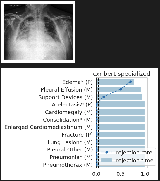
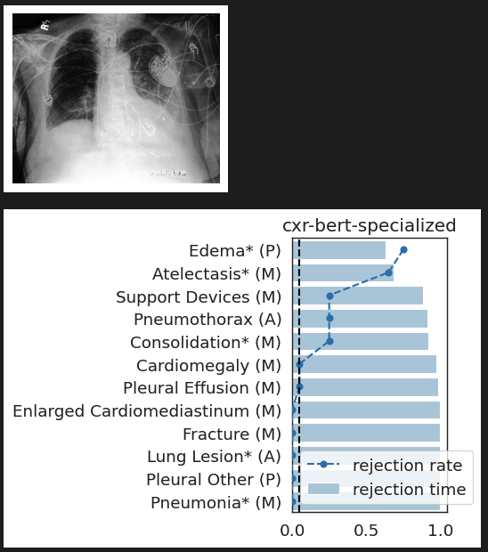
What concepts does BiomedVLP find important to predict ?

lung opacity

Results: RSNA Brain CT Hemorrhage Challenge

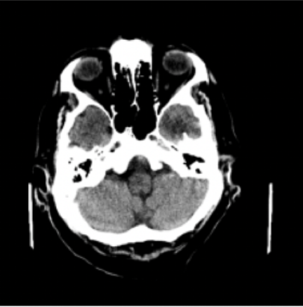
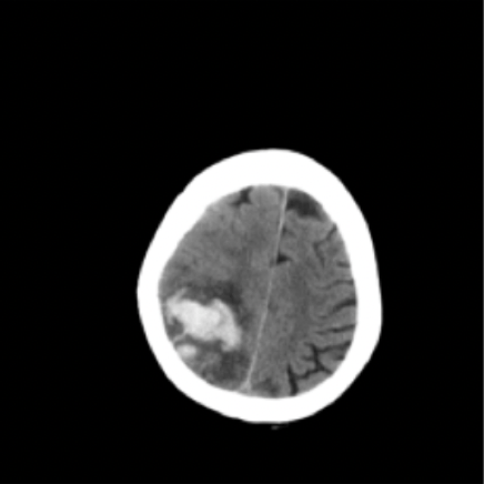
Hemorrhage

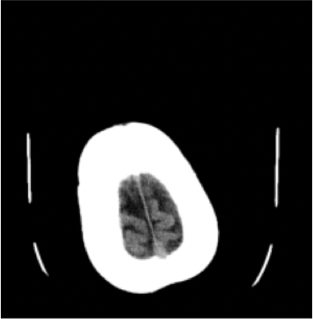
No Hemorrhage

Hemorrhage

Hemorrhage

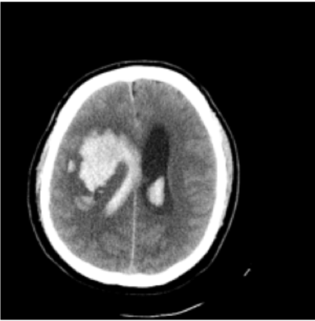
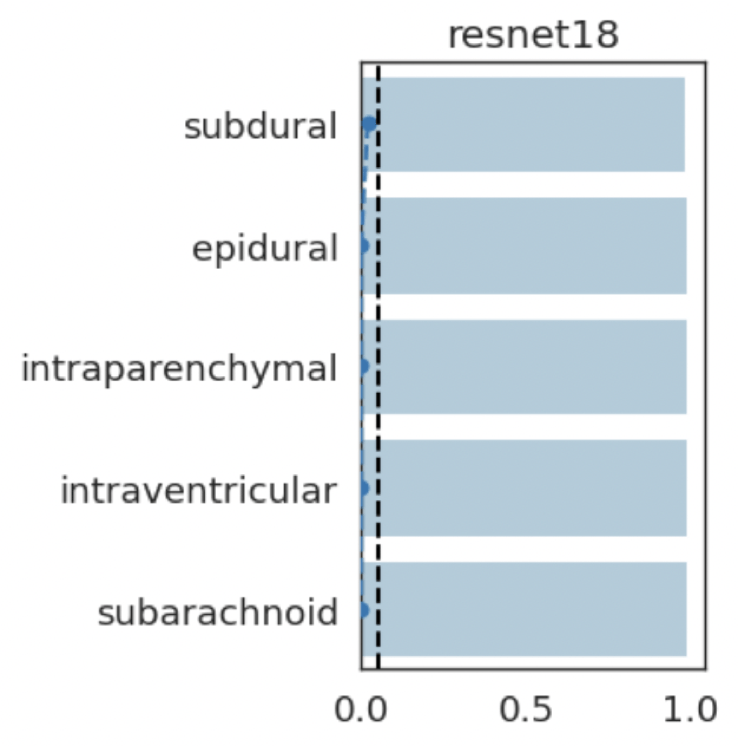
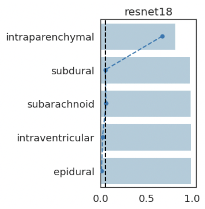
intraparenchymal

subdural

subarachnoid

intraventricular

epidural

intraparenchymal

subarachnoid

intraventricular

epidural

subdural

intraparenchymal

subarachnoid

subdural

epidural

intraventricular

intraparenchymal

subarachnoid

intraventricular

epidural

subdural

(+)

(-)

(-)

(-)

(-)

(+)

(-)

(+)

(-)

(-)

(+)

(+)

(-)

(-)

(-)

(-)

(-)

(-)

(-)

(-)

Results: Imagenette

Global Importance

Results: Imagenette

Global Conditional Importance

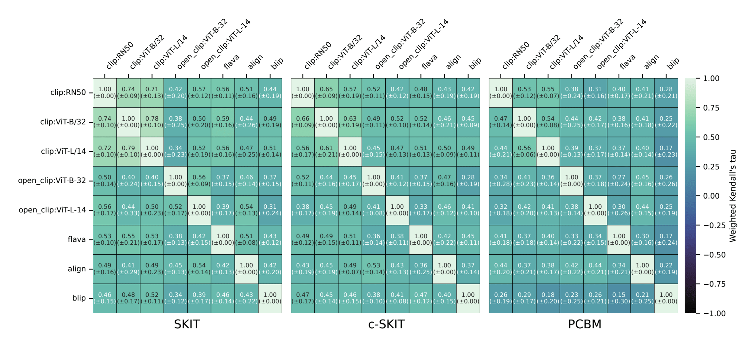
Results: Imagenette

Semantic comparison of vision-language models

Question 1)

Can we resolve the computational bottleneck (and when)?

Question 2)

What do these coefficients mean statistically?

Question 3)

How to go beyond input-features explanations?

Summary

Distributional assumptions + hierarchical extensions

Allow us to conclude on differences in distributions

Use online testing by betting for semantic concepts

CODA: Demographic fairness

Inputs (features): \(X\in\mathcal X \subset \mathbb R^d\)

Responses (labels): \(Y\in\mathcal Y = \{0,1\}\)

Sensitive attributes \(Z \in \mathcal Z \subseteq \mathbb R^k \) (sex, race, age, etc)

\((X,Y,Z) \sim \mathcal D\)

Eg: \(Z_1: \) biological sex, \(X_1: \) BMI, then

\( g(Z,X) = \boldsymbol{1}\{Z_1 = 1 \land X_1 > 35 \}: \) women with BMI > 35

Goal: ensure that \(f\) is fair w.r.t groups \(g \in \mathcal G\)

Demographic fairness

Group memberships \( \mathcal G = \{ g:\mathcal X \times \mathcal Z \to \{0,1\} \} \)

Predictor \( f(X) : \mathcal X \to [0,1]\) (e.g. likelihood of X having disease Y)

Group/Associative Fairness
Predictors should not have very different (error) rates among groups
[Calders et al, '09][Zliobaite, '15][Hardt et al, '16]

Individual Fairness
Similar individuals/patients should have similar outputs
[Dwork et al, '12][Fleisher, '21][Petersen et al, '21]

Causal Fairness
Predictors should be fair in a counter-factual world
[Nabi & Shpitser, '18][Nabi et al, '19][Plecko & Bareinboim, '22]

Multiaccuracy/Multicalibration
Predictors should be approximately unbiased/calibrated for every group
[Kim et al, '20][Hebert-Johnson et al, '18][Globus-Harris et at, 22]

Demographic fairness

Multiaccuracy/Multicalibration
Predictors should be approximately unbiased/calibrated for every group
[Kim et al, '20][Hebert-Johnson et al, '18][Globus-Harris et at, 22]

Demographic fairness

Observation 1:
measuring (& correcting) for MA/MC requires samples over \((X,Y,Z)\)

Definition: \(\text{MA} (f,g) = \big| \mathbb E [ g(X,Z) (f(X) - Y) ] \big| \)

\(f\) is \((\mathcal G,\alpha)\)-multiaccurate if \( \max_{g\in\mathcal G} \text{MA}(f,g) \leq \alpha \)

Definition: \(\text{MC} (f,g) = \mathbb E\left[ \big| \mathbb E [ g(X,Z) (f(X) - Y) | f(X) = v] \big| \right] \)

\(f\) is \((\mathcal G,\alpha)\)-multicalibrated if \( \max_{g\in\mathcal G} \text{MC}(f,g) \leq \alpha \)

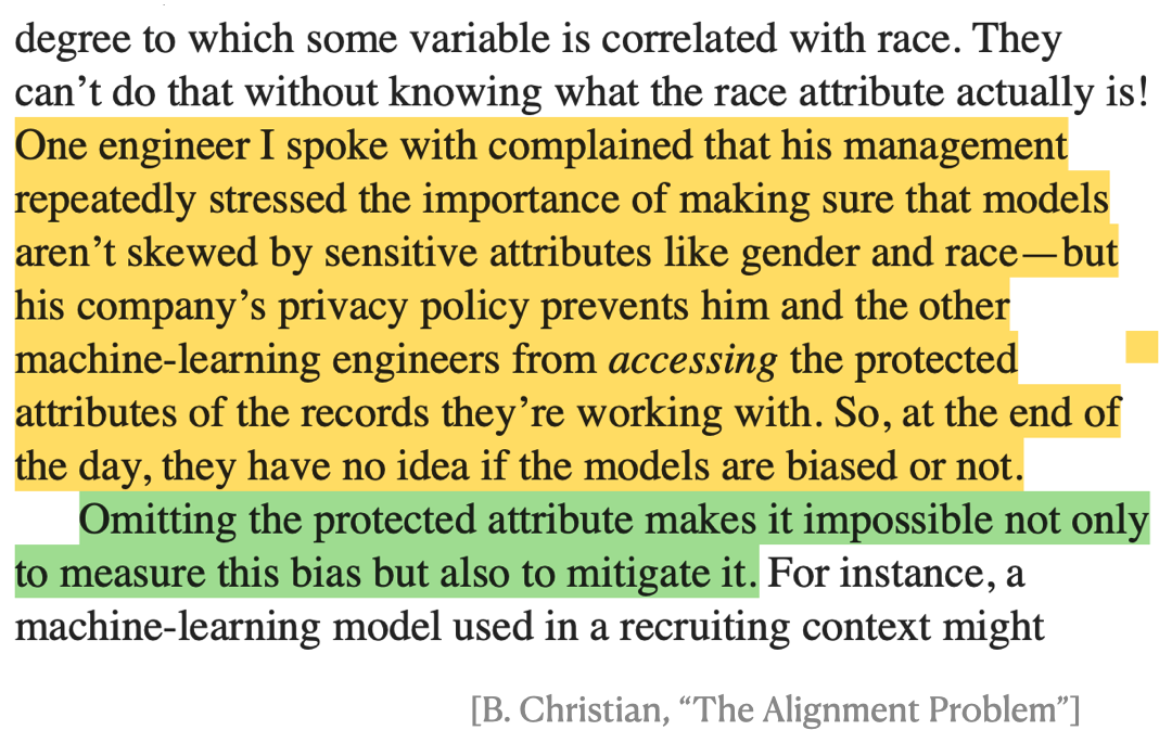
Observation 2: That's not always possible...

sex and race attributes missing

We might want to conceal \(Z\) on purpose, or might need to

We observe samples over \((X,Y)\) to obtain \(\hat Y = f(X)\) for \(Y\)

Fairness in partially observed regimes

\( \text{MSE}(f) = \mathbb E [(Y-f(X))^2 ] \)

A developer provides us with proxies \( \color{Red} \hat{g} : \mathcal X \to \{0,1\} \)

\( \text{err}(\hat g) = \mathbb P [({\color{Red}\hat g(X)} \neq {\color{blue}g(X,Z)} ] \)

[Awasti et al, '21][Kallus et al, '22][Zhu et al, '23][Bharti et al, '24]

Question

Can we (how) use \(\hat g\) to measure (and correct) \( (\mathcal G,\alpha)\)-MA/MC?

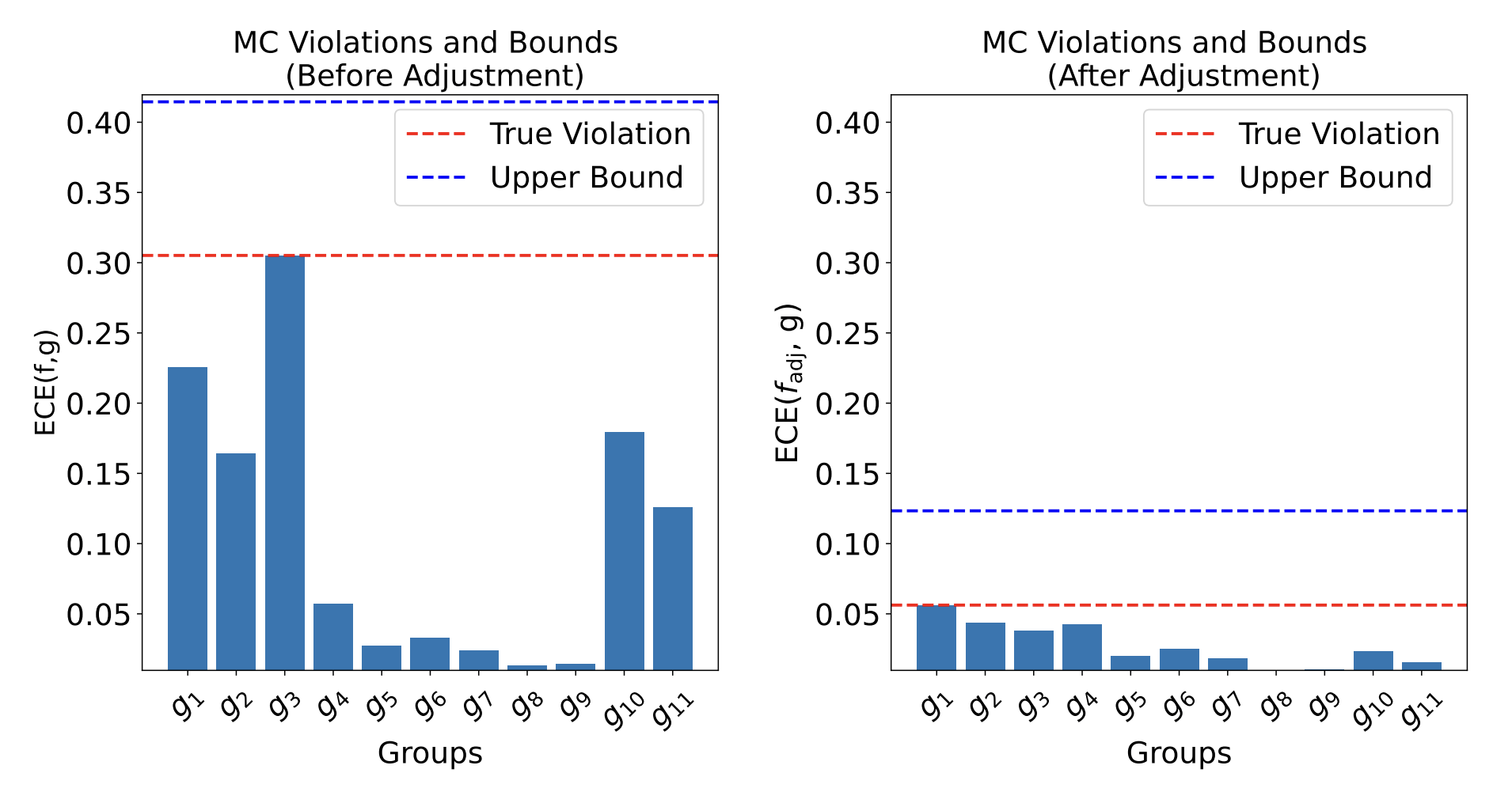
Fairness in partially observed regimes

Theorem [Bharti, Clemens-Sewall, Yi, S.]

With access to \((X,Y)\sim \mathcal D_{\mathcal{XY}}\), proxies \( \hat{\mathcal G}\) and predictor \(f\)

\[ \max_{\color{Blue}g\in\mathcal G} MC(f,{\color{blue}g}) \leq \max_{\color{red}\hat g\in \hat{\mathcal{G}} } B(f,{\color{red}\hat g}) + MC(f,{\color{red}\hat g}) \]

with \(B(f,\hat g) = \min \left( \text{err}(\hat g), \sqrt{MSE(f)\cdot \text{err}(\hat g)} \right) \)

Practical/computable upper bounds \(\)
Multicalibrating w.r.t \(\hat{\mathcal G}\) provably improves upper bound
[Gopalan et al. (2022)][Roth (2022)]

true error

worst-case error

Fairness in partially observed regimes

CheXpert: Predicting abnormal findings in chest X-rays
(not accessing race or biological sex)

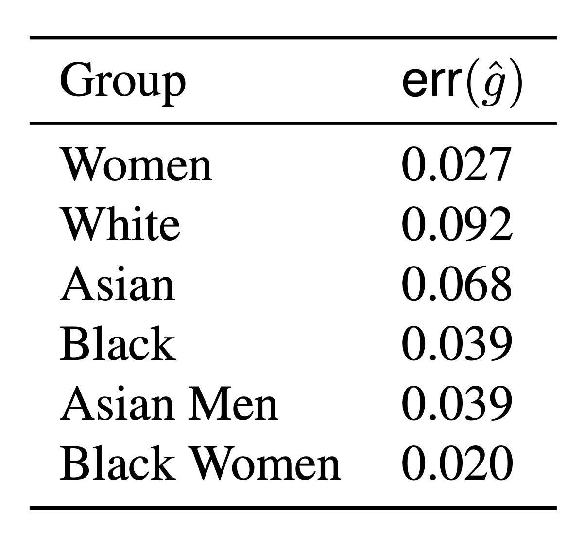
\(f(X): \) likelihood of \(X\) having \(\texttt{pleural effusion}\)

Demographic fairness

Take-home message

Proxies can be very useful in certifying max. fairness violations
Can allow for simple post-processing corrections

Jacopo Teneggi
JHU

Beepul Bharti
JHU

Teneggi et al, SHAP-XRT: The Shapley Value Meets Conditional Independence Testing, TMLR (2023).

Teneggi et al, Fast hierarchical games for image explanations, Teneggi, Luster & S., IEEE TPAMI (2022)

Teneggi & S., Testing Semantic Importance via Betting, Neurips (2024).

Yaniv Romano Technion

Bharti et al, Multiaccuracy and Multicalibration via Proxy Groups, 
ICML (2025).

Recent advances in trustworthy machine learning for computational imaging

Jeremias Sulam

Interpretability in Image Classification

Sensitivity or Gradient-based perturbations

Shapley coefficients

Variational formulations

Counterfactual & causal explanations

LIME [Ribeiro et al, '16], CAM [Zhou et al, '16], Grad-CAM [Selvaraju et al, '17]

Shap [Lundberg & Lee, '17], ...

RDE [Macdonald et al, '19], ...

[Sani et al, 2020] [Singla et al '19],..

Post-hoc Interpretability in Image Classification

Sensitivity or Gradient-based perturbations

Shapley coefficients

Variational formulations

Counterfactual & causal explanations

LIME [Ribeiro et al, '16], CAM [Zhou et al, '16], Grad-CAM [Selvaraju et al, '17]

Shap [Lundberg & Lee, '17], ...

RDE [Macdonald et al, '19], ...

[Sani et al, 2020] [Singla et al '19],..

Post-hoc Interpretability in Image Classification

Adebayo et al, Sanity checks for saliency maps, 2018

Ghorbani et al, Interpretation of neural networks is fragile, 2019

Shah et al, Do input gradients highlight discriminative features? 2021

Sensitivity or Gradient-based perturbations

Shapley coefficients

Variational formulations

Counterfactual & causal explanations

LIME [Ribeiro et al, '16], CAM [Zhou et al, '16], Grad-CAM [Selvaraju et al, '17]

Shap [Lundberg & Lee, '17], ...

RDE [Macdonald et al, '19], ...

[Sani et al, 2020] [Singla et al '19],..

Post-hoc Interpretability in Image Classification

Adebayo et al, Sanity checks for saliency maps, 2018

Ghorbani et al, Interpretation of neural networks is fragile, 2019

Shah et al, Do input gradients highlight discriminative features? 2021

Sensitivity or Gradient-based perturbations

Shapley coefficients

Variational formulations

Counterfactual & causal explanations

LIME [Ribeiro et al, '16], CAM [Zhou et al, '16], Grad-CAM [Selvaraju et al, '17]

Shap [Lundberg & Lee, '17], ...

RDE [Macdonald et al, '19], ...

[Sani et al, 2020] [Singla et al '19],..

Post-hoc Interpretability in Image Classification

Adebayo et al, Sanity checks for saliency maps, 2018

Ghorbani et al, Interpretation of neural networks is fragile, 2019

Shah et al, Do input gradients highlight discriminative features? 2021

marginal contribution of player i with coalition S

Shapley values

Shap-Explanations

Shap-Explanations

Shap-Explanations

Shap-Explanations

Guiding Questions

Hierarchical Shap (h-Shap)

Theorem (informal)

Hierarchical Shap (h-Shap)

Hierarchical Shap (h-Shap)

Hierarchical Shap (h-Shap)

Other notions of structure

Other notions of structure

Precise notions of importance

Formal Feature Importance

Precise notions of importance

How do we test?

Local Feature Importance

Precise notions of importance

Local Feature Importance

Semantic Interpretability of classifiers

model-agnostic interpretability

Semantic Interpretability of classifiers

Semantic Interpretability of classifiers

Semantic Interpretability of classifiers

Semantic Interpretability of classifiers

Concept Bottleneck Models (CMBs)

Precise notions of semantic importance

Precise notions of semantic importance

Precise notions of semantic importance

Precise notions of semantic importance