Modern problems in Biomedical Imaging

2026 Workshop on MR Phase, Magnetic Susceptibility and Electrical Properties Mapping

Jeremias Sulam

50 years ago ...

first CT scan

ELECTRIC & MUSICAL INDUSTRIES

50 years ago ...

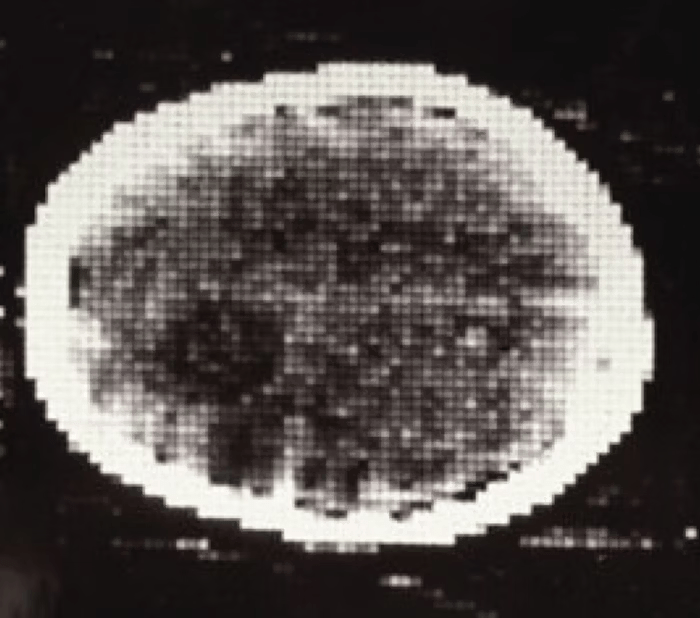
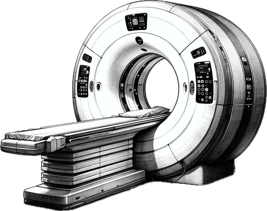
imaging

diagnostics

complete hardware & software description

human expert diagnosis and recommendations

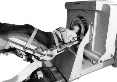
imaging was "simple"

... 50 years forward

Data

Compute & Hardware

Sensors & Connectivity

Research & Engineering

... 50 years forward

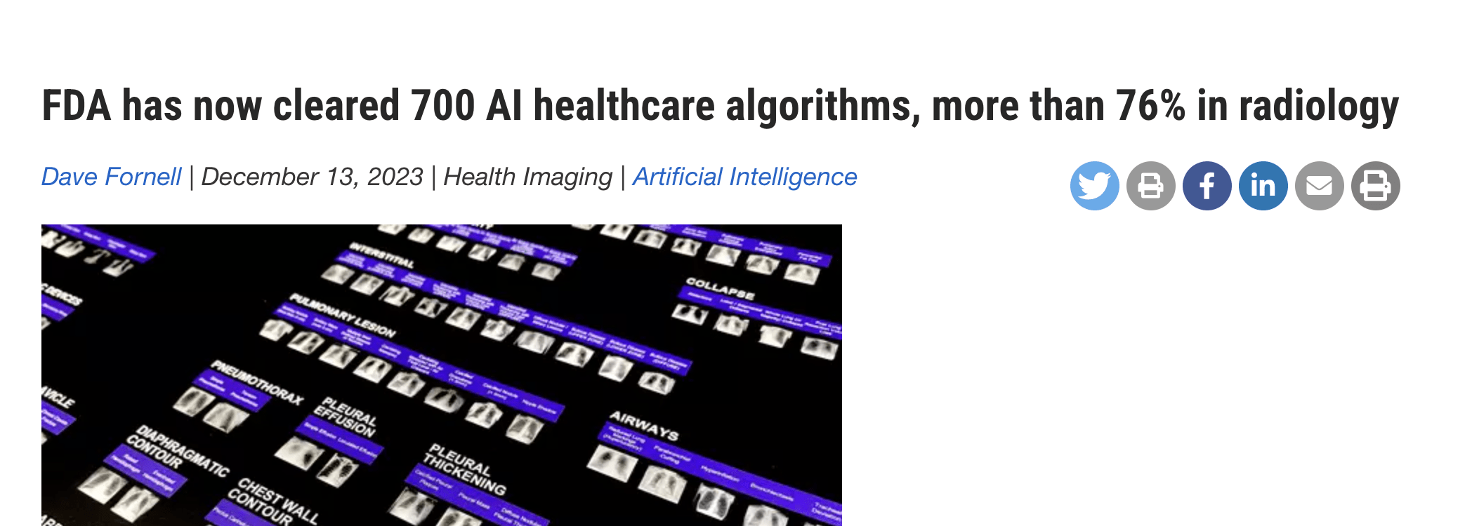
data-driven  imaging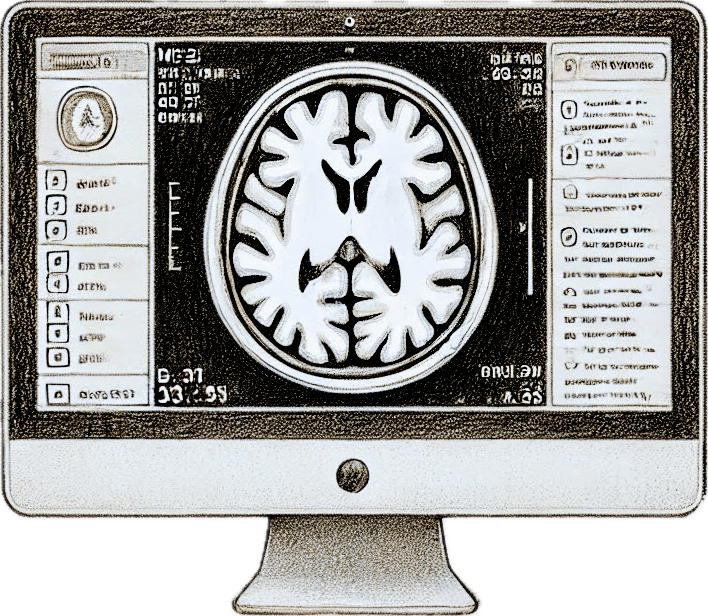

automatic analysis and rec.

societal implications

Data

Compute & Hardware

Sensors & Connectivity

Research & Engineering

data-driven  imaging

automatic analysis and rec.

societal implications

Problems in trustworthy biomedical imaging

inverse problems

uncertainty quantification

robustness

generalization

demographic fairness

hardware & protocol optimization

model-agnostic interpretability

policy & regulation

monitoring & auditing

data-driven  imaging

automatic analysis and rec.

societal implications

Problems in trustworthy biomedical imaging

inverse problems

uncertainty quantification

robustness

generalization

demographic fairness

hardware & protocol optimization

model-agnostic interpretability

policy & regulation

monitoring & auditing

$x\sim p_x$

$z\sim \mathcal N(0,\sigma^2 I)$

$y = x + z$

$x\sim p_x$

$z\sim \mathcal N(0,\sigma^2 I)$

$A~\cdot$

$y = Ax + z$

estimate

Inverse Problems

$= \underset{x}{\arg\max} ~~~ p(y|x)p_x(x)$

$= \underset{x}{\arg\min} ~ -\log p(y|x) - \log p_x(x)$

$= \underset{x}{\arg\min} ~ \frac{1}{2\sigma^2} \|y-x\|^2_2 - \log p_x(x)$

$\hat{x} = \underset{x}{\arg\max} ~ p(x|y)$

Maximum a

Posteriori

estimator

MAP

likelihood

prior

$= \text{prox}_{-\sigma^2 \log p_x}(y)$

Inverse Problems

$x\sim p_x$

$z\sim \mathcal N(0,\sigma^2 I)$

$y = x + z$

Inverse Problems

$x\sim p_x$

$z\sim \mathcal N(0,\sigma^2 I)$

$y = A x + z$

$A~ \cdot$

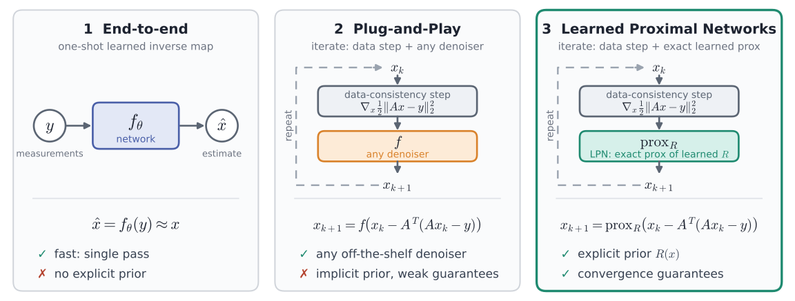
Inverse Problems

$x\sim p_x$

$z\sim \mathcal N(0,\sigma^2 I)$

$y = A x + z$

$A~ \cdot$

Inverse Problems

$x\sim p_x$

$z\sim \mathcal N(0,\sigma^2 I)$

$y = A x + z$

$A~ \cdot$

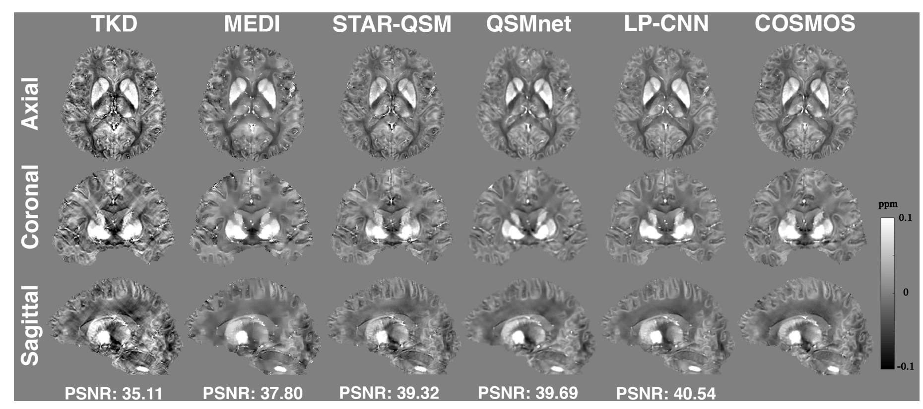
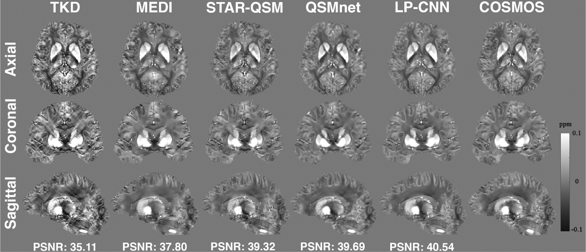
Quantitative Susceptibility Mapping

[Lai, Kuo-Wei, et al. "Learned proximal networks for quantitative susceptibility mapping." International Conference on Medical Image Computing and Computer-Assisted Intervention. Cham: Springer International Publishing, 2020.]

[Fang, Zhenghan, et al. "DeepSTI: Towards tensor reconstruction using fewer orientations in susceptibility tensor imaging." Medical image analysis 87 (2023): 102829.]

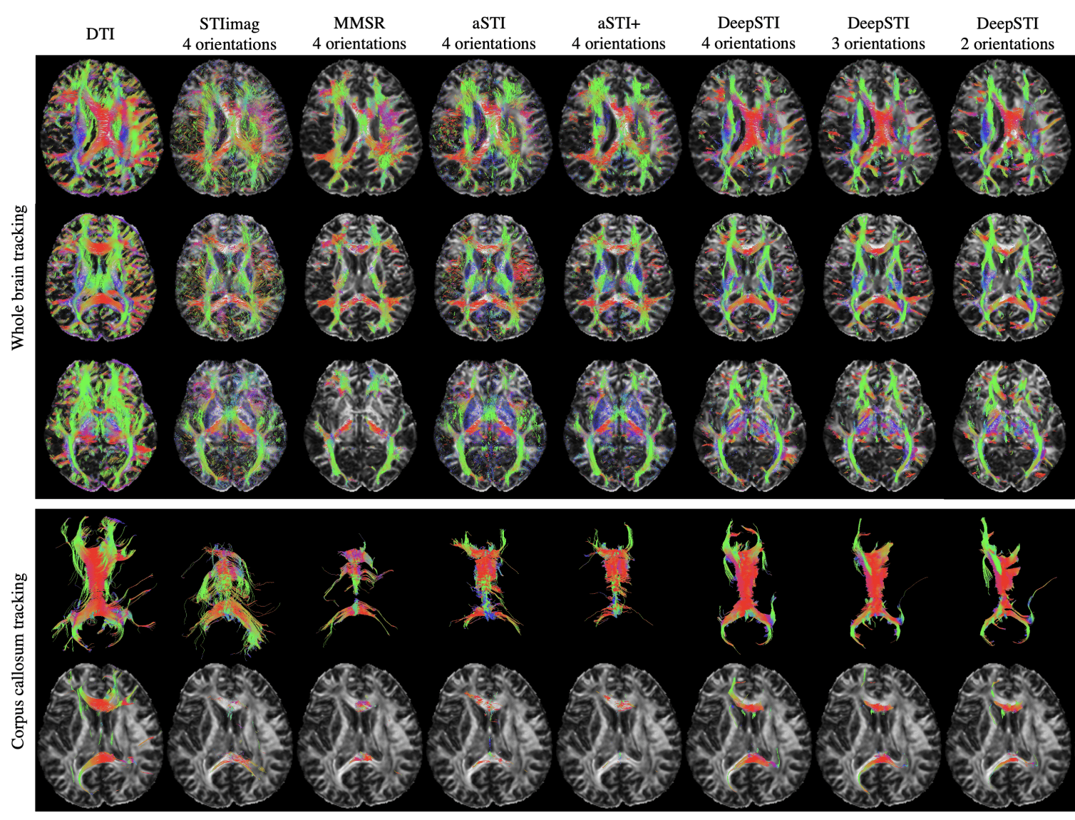
Susceptibility Tensor Imaging

[Fang, Zhenghan, et al. "DeepSTI: Towards tensor reconstruction using fewer orientations in susceptibility tensor imaging." Medical image analysis 87 (2023): 102829.]

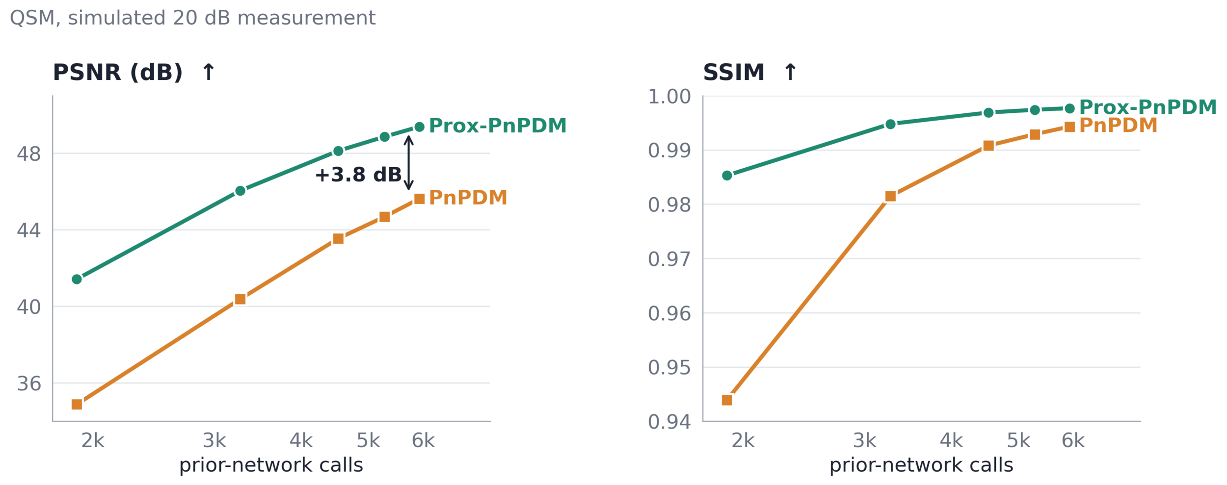
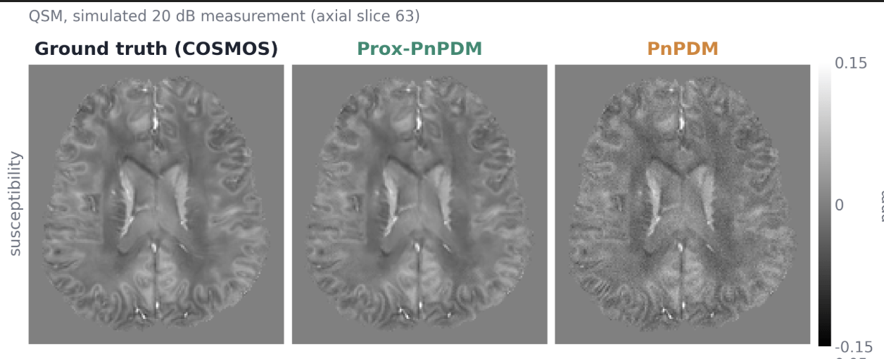
Conditional (Prox) Diffusion Sampling

baseline

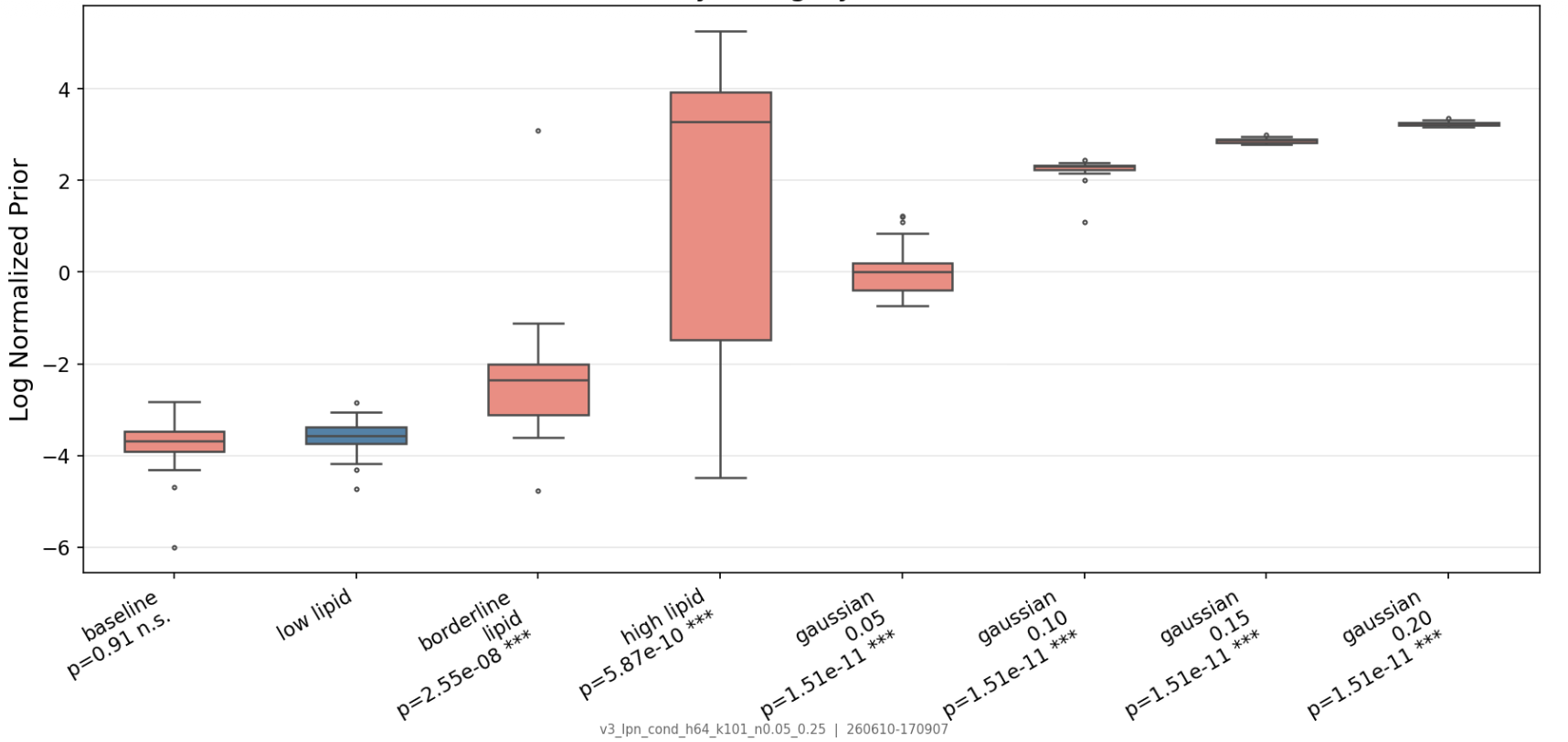
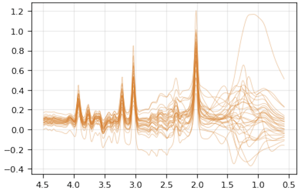
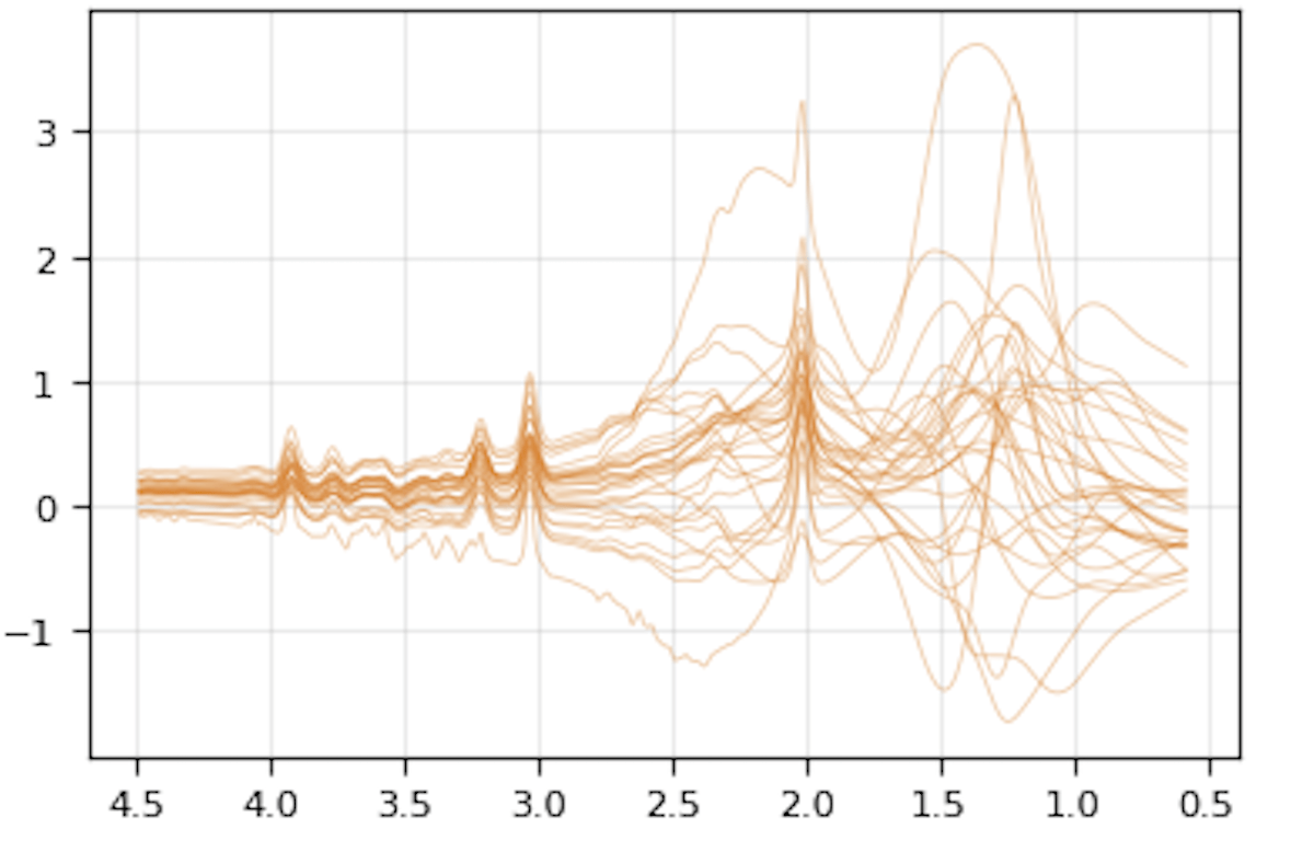
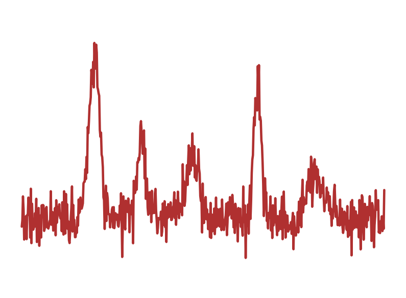
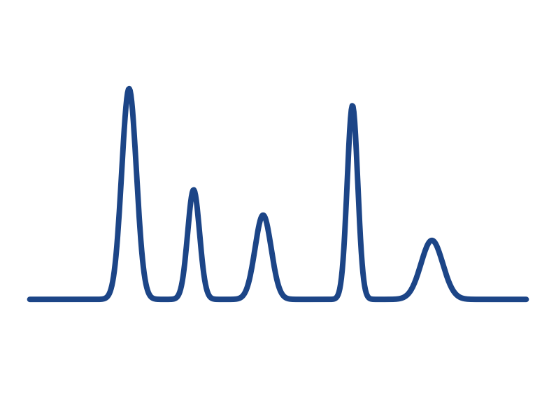
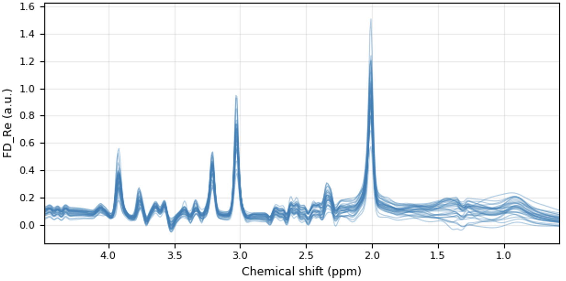
Priors for MR Spectroscopy

data-driven  imaging

automatic analysis and rec.

societal implications

Problems in trustworthy biomedical imaging

inverse problems

uncertainty quantification

robustness

generalization

demographic fairness

hardware & protocol optimization

model-agnostic interpretability

policy & regulation

monitoring & auditing

in a box

Denoiser

Measurements

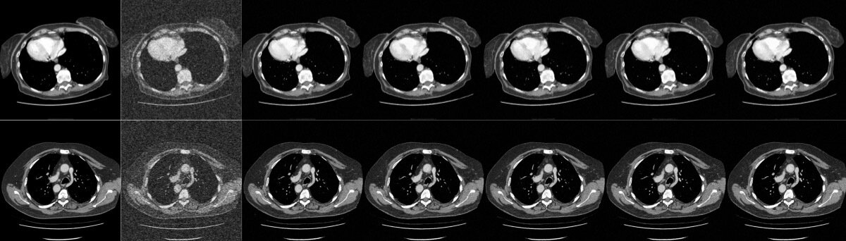
Reconstruction

Uncertainty Quantification

$\hat{x} = f_\theta(y)$

$\text{pixel}_j$

$\hat{x}_j$

(point predictors)

What is the uncertainty in the guess $\hat x_j$ ?

How do we report uncertainty rigorously?

$y = Ax + z$

Measurements

$\hat{X} = F(y) \sim \mathcal{P}_y$

Sampling

$\text{pixel}_j$

$\hat{x}_j$

(predictive distribution)

What is the uncertainty in the guess $\hat x_j$ ?

How do we report uncertainty rigorously?

Uncertainty Quantification

$y = Ax + z$

in a box

Denoiser

$0$

$1$

$l(y)_j$

$u(y)_j$

Uncertainty through Prediction Sets

How do we construct them?

pixel-wise mean $\pm$ standard deviation
Quantile regression
MC-dropout (Gal & Ghahramani, 2016)
any other heuristics...

$C: y \mapsto C(y) \subseteq [0,1]^d$

$\mathcal C(y)_j = [l(y)_j,u(y)_j]$

Miscoverage:

$\ell(y,x) = \frac{1}{d} \sum_{j\in[d]} \mathbf{1}\!\left\{x_j \notin C(y)_j\right\}$

$0$

$1$

$l(y)_j$

$u(y)_j$

Uncertainty through Prediction Sets

$C: y \mapsto C(y) \subseteq [0,1]^d$

ground truth!

$x_j$

$0$

$1$

$l(y)_j$

$\mathcal C(y)_j$

$u(y)_j$

$\lambda$

$C(y)_j = [l_j(y),u_j(y)] \;\longrightarrow\; C_{\lambda}(y)_j = [l_j(y)-{\color{green}{\lambda}},\;u_j(y)+{\color{green}\lambda}]$

Uncertainty through Prediction Sets

Given a calibration set $S_\text{cal} = \{x_i,y_i\},$ provides a simple procedure so that

$\mathbb{E} [\ell(C(y),x))]\leq \epsilon $

(distribution free!)

Conformal Risk Control:

[Angelopoulos et al, 2024]

$C_{\lambda}(y)_j = [l_j(y)-{\color{green}{\lambda}},\;u_j(y)+{\color{green}\lambda}]$

Observation 1: Single $\lambda$ for all $d$ dimensions... suboptimal

Uncertainty through Prediction Sets

$C_{\lambda}(y)_j = [l_j(y)-{\color{green}{\lambda}},\;u_j(y)+{\color{green}\lambda}]$

Observation 1: Single $\lambda$ for all $d$ dimensions... suboptimal

Observation 2: High-dim data is heterogenous

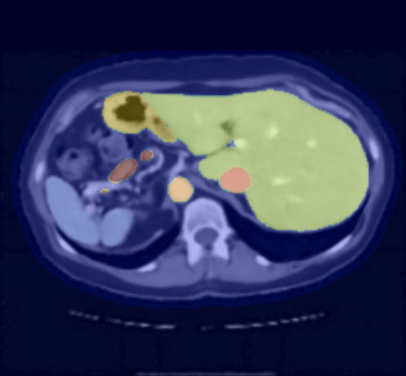
$C_{\lambda}(y)_j = [l_j(y)-{\color{green}{\lambda_j}},\;u_j(y)+{\color{green}\lambda_j}]$

$\lambda_j$ for each $j^\text{th}$ organ

Uncertainty through Prediction Sets

Semantic Uncertainty Quantification

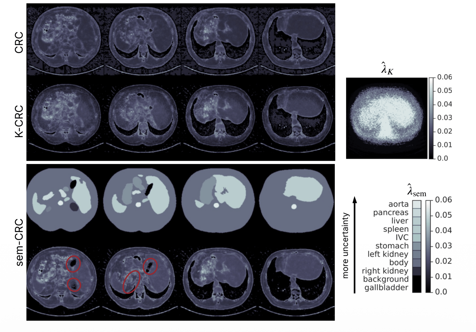
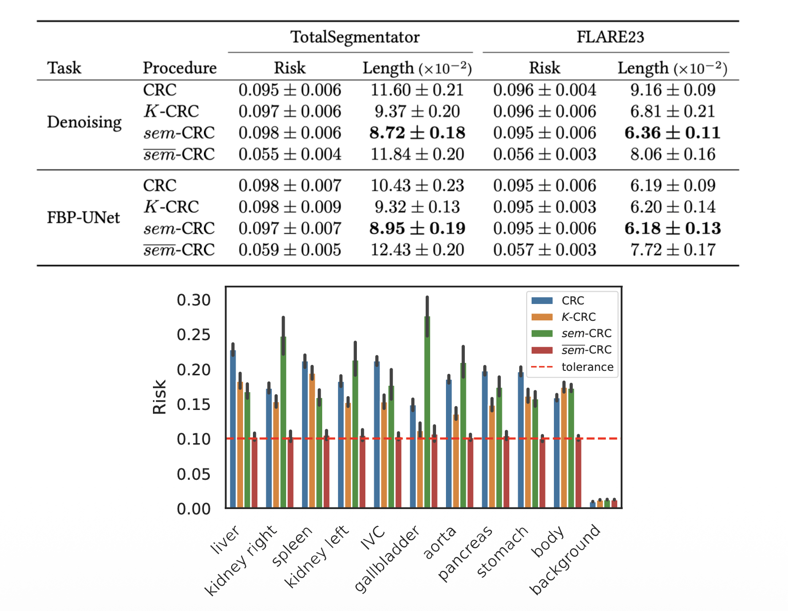
risk controlled uniformly for every organ

[Teneggi, Jacopo, J. Webster Stayman, and Jeremias Sulam. "Conformal risk control for semantic uncertainty quantification in computed tomography." MICCAI , 2025.]

data-driven  imaging

automatic analysis and rec.

societal implications

Problems in trustworthy biomedical imaging

inverse problems

uncertainty quantification

robustness

generalization

demographic fairness

hardware & protocol optimization

model-agnostic interpretability

policy & regulation

monitoring & auditing

Acknowledgements

Jacopo Teneggi

Zhenghan Fang

Yuqing He

Xu Li

Peter van Zijl

Georg Oeltzschner

Chris Davies-Jenkins

policy & regulation

robustness

generalization

uncertainty quantification

Mathematical tractability vs Complexity

in a box

simpler models

more assumptions

any model

no assumptions

Denoiser

Linear models

Linear networks

Shallow

ReLU Networks

Just ask GPT

Conformal guarantees

Modern problems in Biomedical Imaging

2026 Workshop on MR Phase, Magnetic Susceptibility and Electrical Properties Mapping

Jeremias Sulam

50 years ago ...

50 years ago ...

complete hardware & software description

human expert diagnosis and recommendations

imaging was "simple"

... 50 years forward

Data

Compute & Hardware

Sensors & Connectivity

Research & Engineering

... 50 years forward

Data

Compute & Hardware

Sensors & Connectivity

Research & Engineering

Problems in trustworthy biomedical imaging

inverse problems

uncertainty quantification

robustness

generalization

demographic fairness

hardware & protocol optimization

model-agnostic interpretability

policy & regulation

monitoring & auditing

Problems in trustworthy biomedical imaging

inverse problems

uncertainty quantification

robustness

generalization

demographic fairness

hardware & protocol optimization

model-agnostic interpretability

policy & regulation

monitoring & auditing

Inverse Problems

\(\hat{x} = \underset{x}{\arg\max} ~ p(x|y)\)

MAP

Inverse Problems

Inverse Problems

Inverse Problems

Inverse Problems

Quantitative Susceptibility Mapping

Susceptibility Tensor Imaging

Conditional (Prox) Diffusion Sampling

Priors for MR Spectroscopy

Problems in trustworthy biomedical imaging

inverse problems

uncertainty quantification

robustness

generalization

demographic fairness

hardware & protocol optimization

model-agnostic interpretability

policy & regulation

monitoring & auditing

in a box

Denoiser

Measurements

Reconstruction

Uncertainty Quantification

Measurements

Sampling

Uncertainty Quantification

in a box

Denoiser

Uncertainty through Prediction Sets

How do we construct them?

Miscoverage:

Uncertainty through Prediction Sets

Uncertainty through Prediction Sets

Conformal Risk Control:

Uncertainty through Prediction Sets

Uncertainty through Prediction Sets

Semantic Uncertainty Quantification

Problems in trustworthy biomedical imaging

inverse problems

Bayesian

MC Dropout