From Data to Insights
Jeremias Sulam
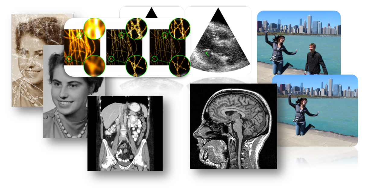
Trustworthy methods for modern biomedical imaging


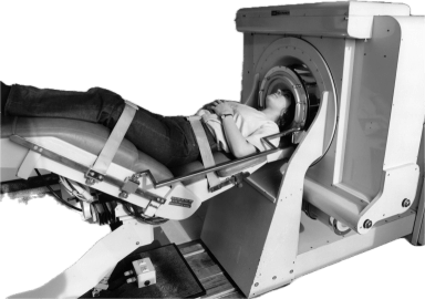
50 years ago ...
first CT scan


ELECTRIC & MUSICAL INDUSTRIES
50 years ago ...
imaging
diagnostics
complete hardware & software description
human expert diagnosis and recommendations
imaging was "simple"
... 50 years forward

Data

Compute & Hardware


Sensors & Connectivity


Research & Engineering
... 50 years forward
Data
Compute & Hardware
Sensors & Connectivity
Research & Engineering


data-driven imaging
automatic analysis and rec.
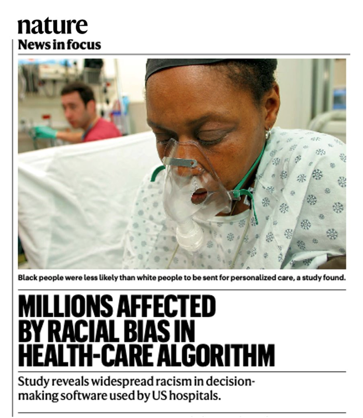
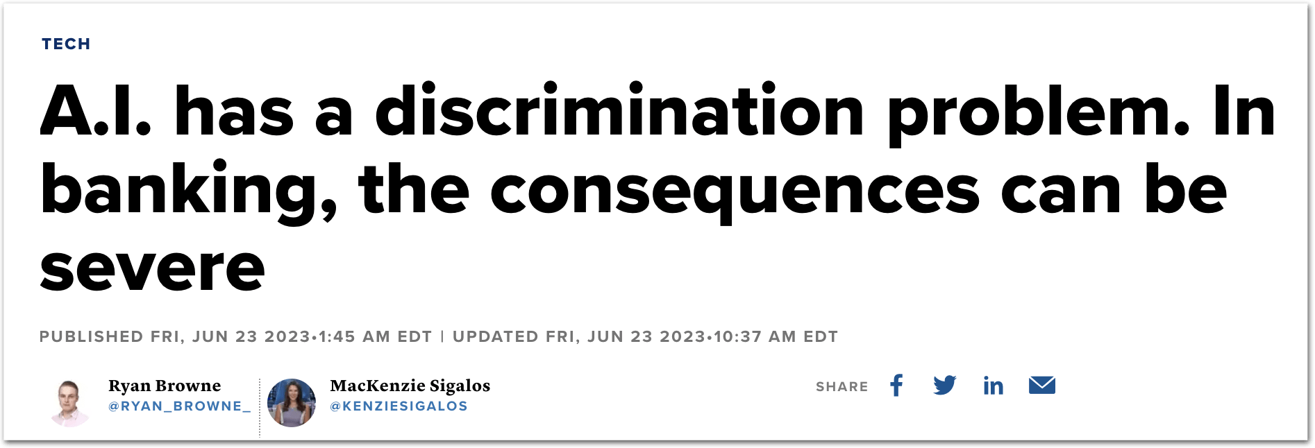
societal implications


Data
Compute & Hardware
Sensors & Connectivity
Research & Engineering


... 50 years forward
data-driven imagingautomatic analysis and rec.societal implicationsProblems in trustworthy biomedical imaging
inverse problems
uncertainty quantification
model-agnostic interpretability
robustness
generalization
policy & regulation
Demographic fairness
hardware & protocol optimization
inverse problems
uncertainty quantification
model-agnostic interpretability
robustness
generalization
policy & regulation
Demographic fairness
hardware & protocol optimization
data-driven imaging
automatic analysis and rec.
societal implications
Problems in trustworthy biomedical imaging
measurements
reconstruction
inverse problems
measurements
reconstruction

inverse problems
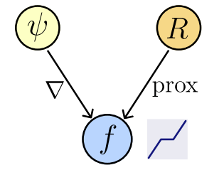
Proximal Gradient Descent: \( x^{t+1} = \text{prox}_R \left(x^t - \eta A^\top(Ax^t-y)\right) \)
... a denoiser
\({\color{red}f_\theta}\): off-the-shelf denoiser
[Venkatakrishnan et al., 2013; Zhang et al., 2017b; Meinhardt et al., 2017; Zhang et al., 2021; Gilton, Ongie, Willett, 2019; Kamilov et al., 2023b; Terris et al., 2023; S Hurault et al. 2021, Ongie et al, 2020; ...]
Plug and Play: Implicit Priors
Question 1)
What are these black-box functions computing? and what have they learned about the data?
Theorem [Fang, Buchanan, S.]
When will \(f_\theta(x)\) compute a \(\text{prox}_R(x)\), and for what \(R(x)\)?
Let \(f_\theta : \mathbb R^n\to\mathbb R^n\) be a network : \(f_\theta (x) = \nabla \psi_\theta (x)\),
where \(\psi_\theta : \mathbb R^n \to \mathbb R,\) convex and differentiable (ICNN).
Then,
1. Existence of regularizer
\(\exists ~R_\theta : \mathbb R^n \to \mathbb R\) not necessarily convex : \(f_\theta(x) \in \text{prox}_{R_\theta}(x),\)
2. Computability
We can compute \(R_{\theta}(x)\) by solving a convex problem
Learned Proximals
: revisiting PnP
How do we find \(f(x) = \text{prox}_R(x)\) for the "correct" \(R(x) \propto -\log p_x(x)\)?
Learned Proximals
: revisiting PnP
Theorem [Fang, Buchanan, S.]
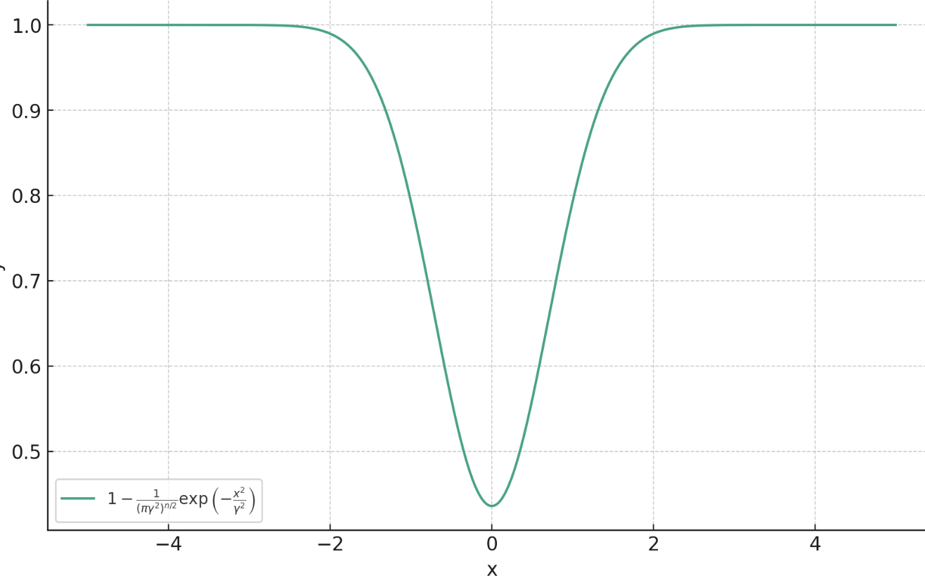
Proximal Matching Loss:\(\gamma\)
Goal: train a denoiser \(f(y)\approx x\)
Let
Then,
a.s.
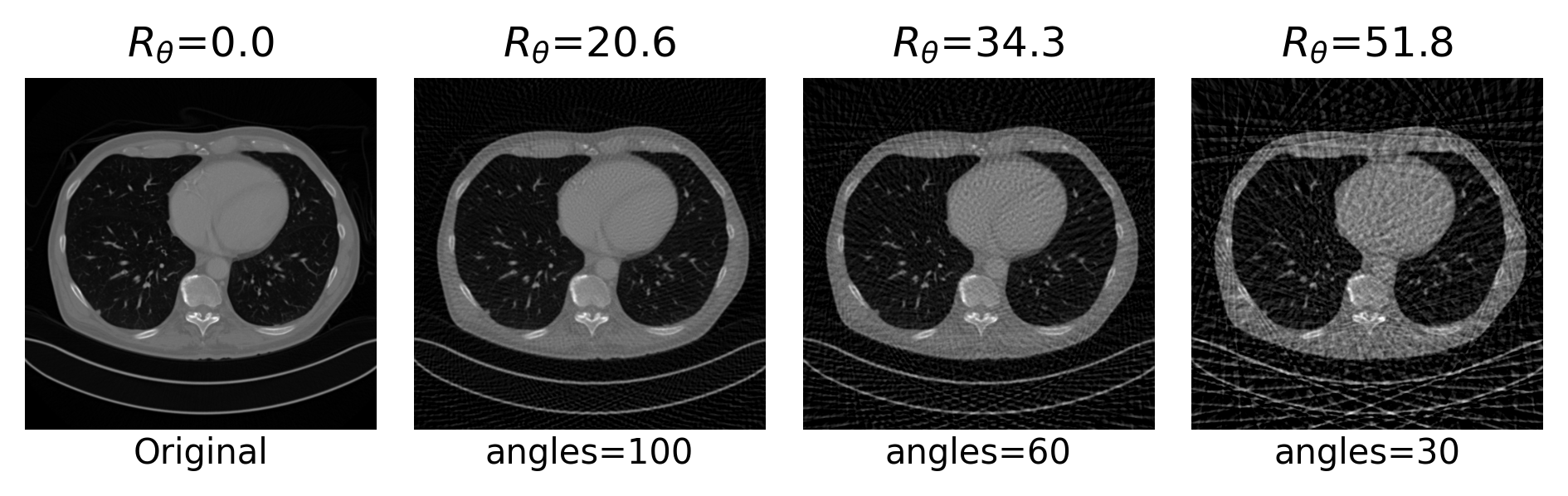
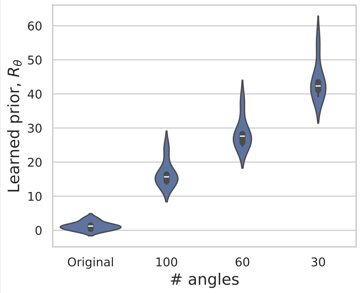
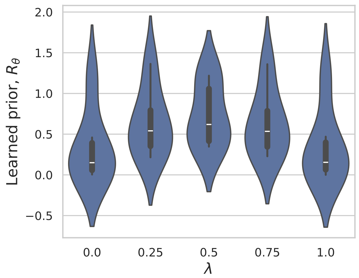
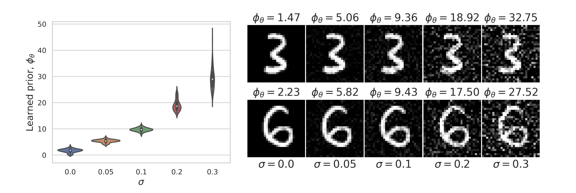
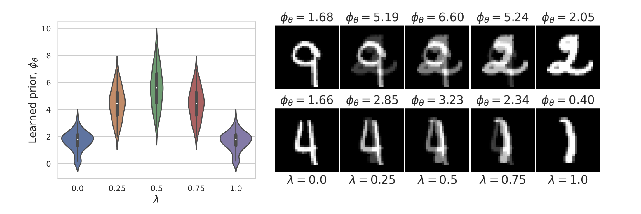
Learned Proximal Networks
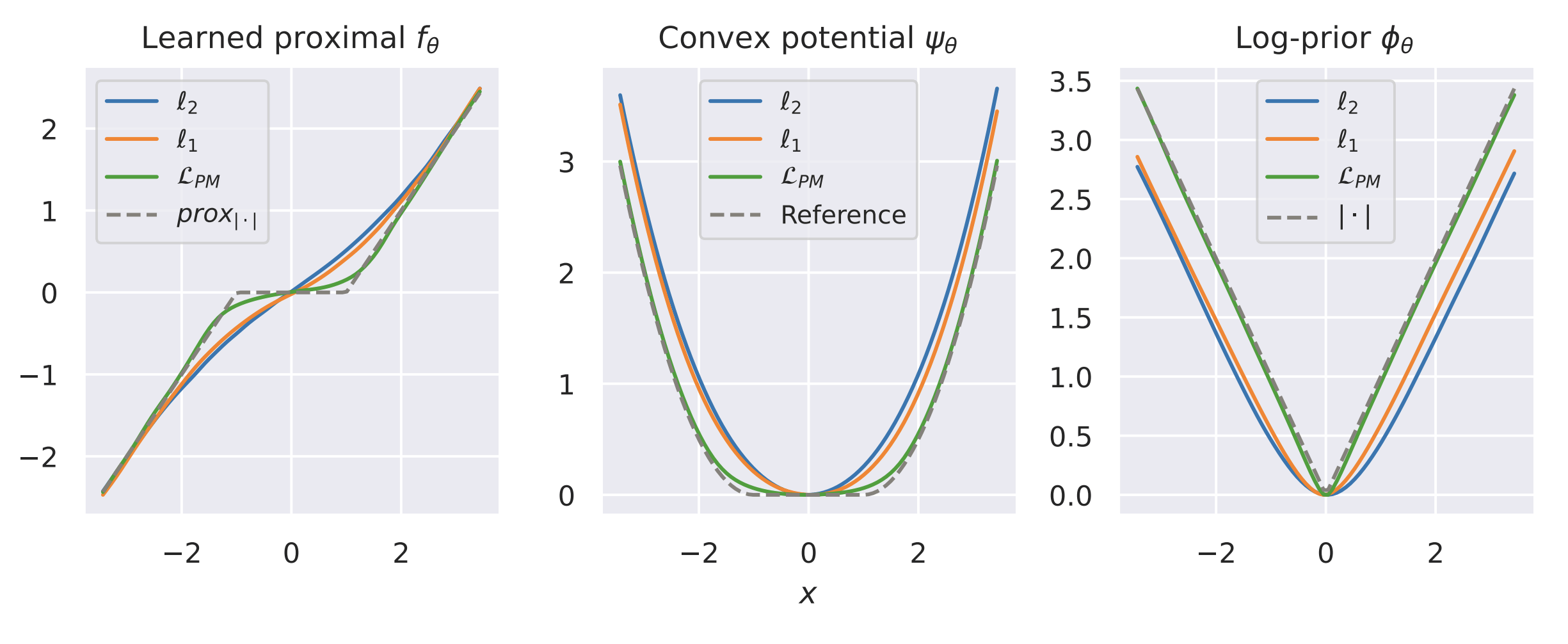
Example: recovering a prior
Fang, Buchanan & S. What's in a Prior? Learned Proximal Networks for Inverse Problems, ICLR 2024.
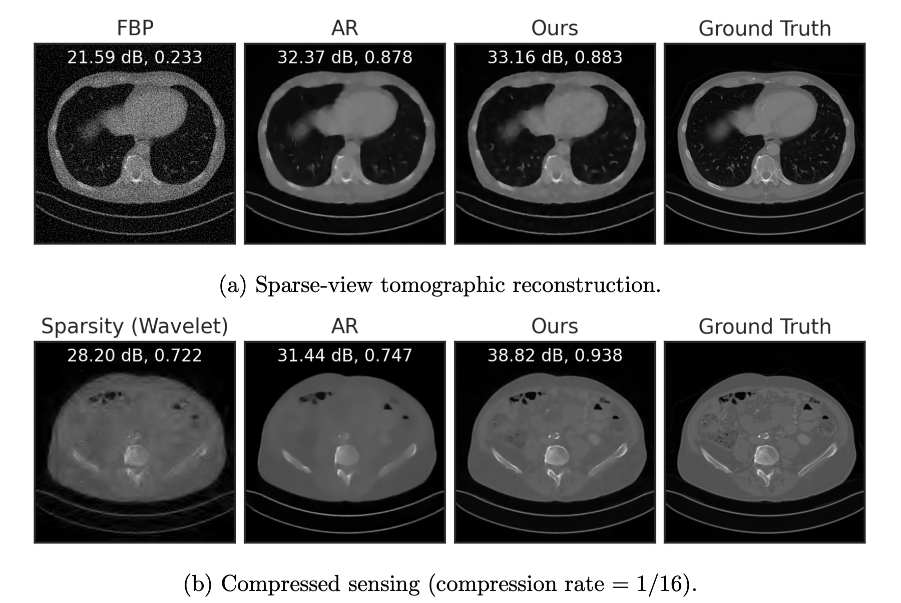
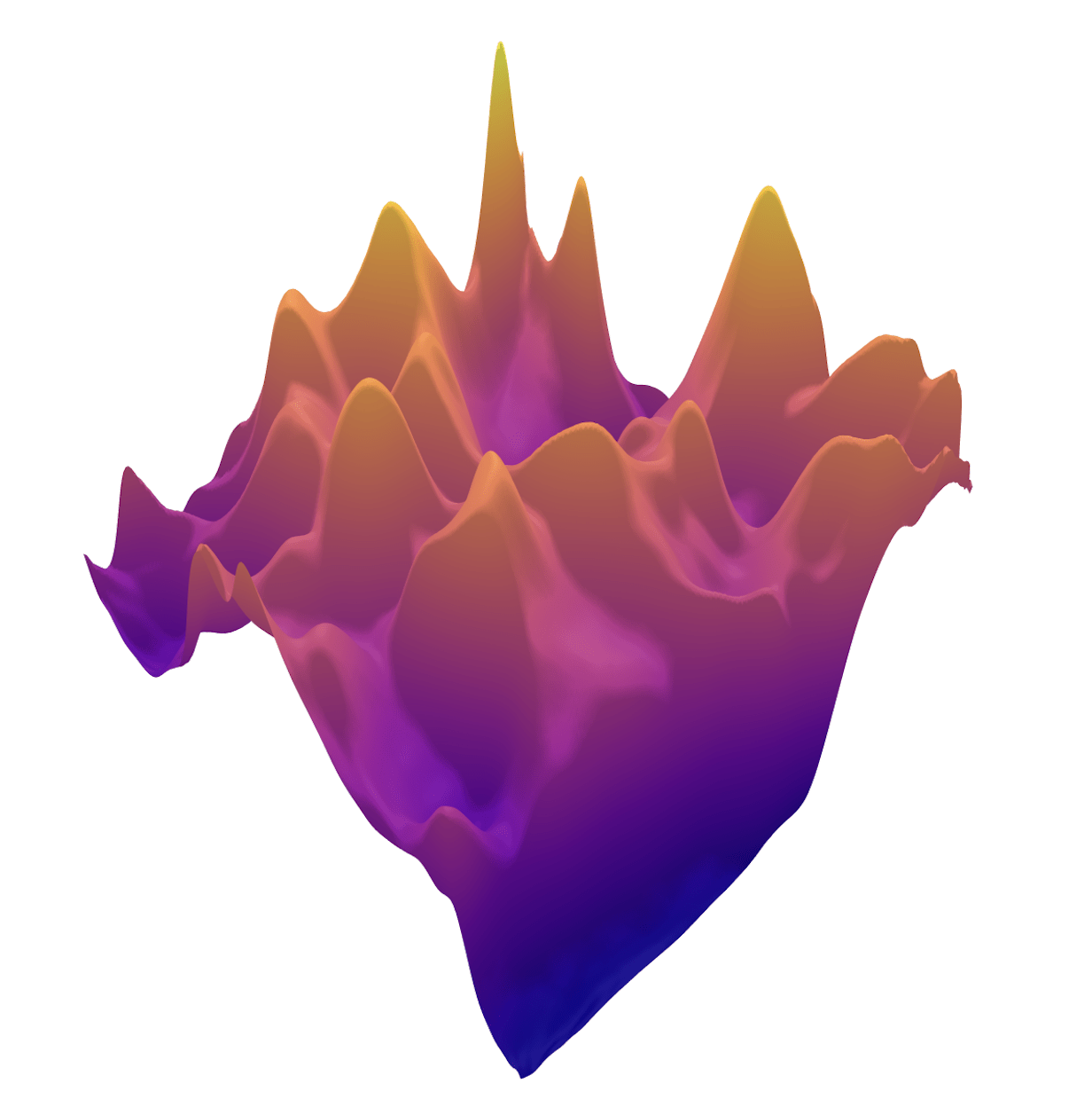
Learned Proximal Networks in
Convergence guarantees
inverse problems
Fang, Buchanan & S. What's in a Prior? Learned Proximal Networks for Inverse Problems, ICLR 2024.
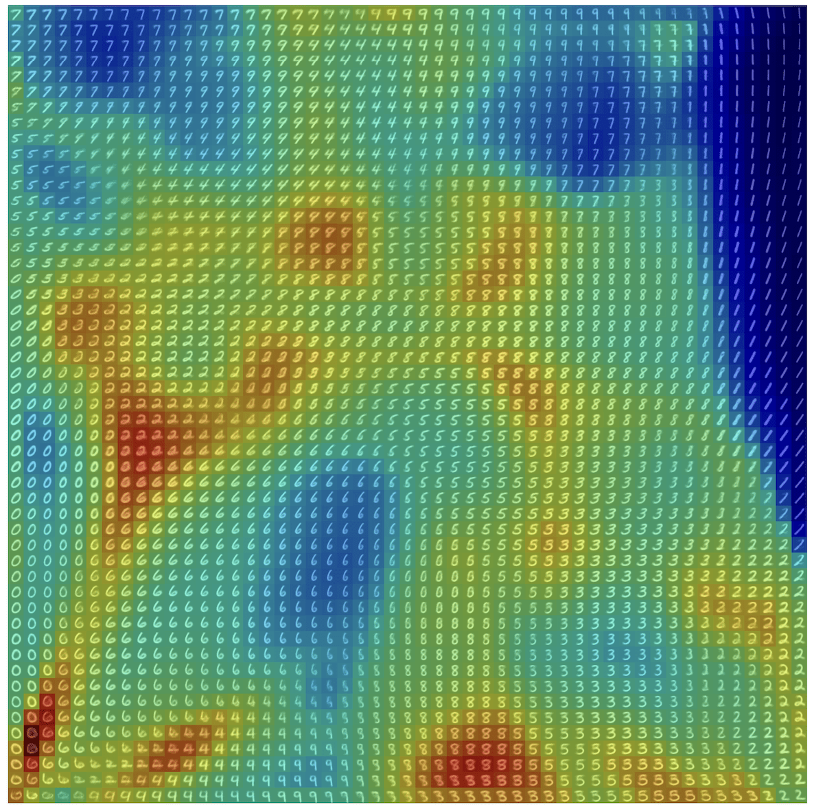
Learned Proximal Networks in
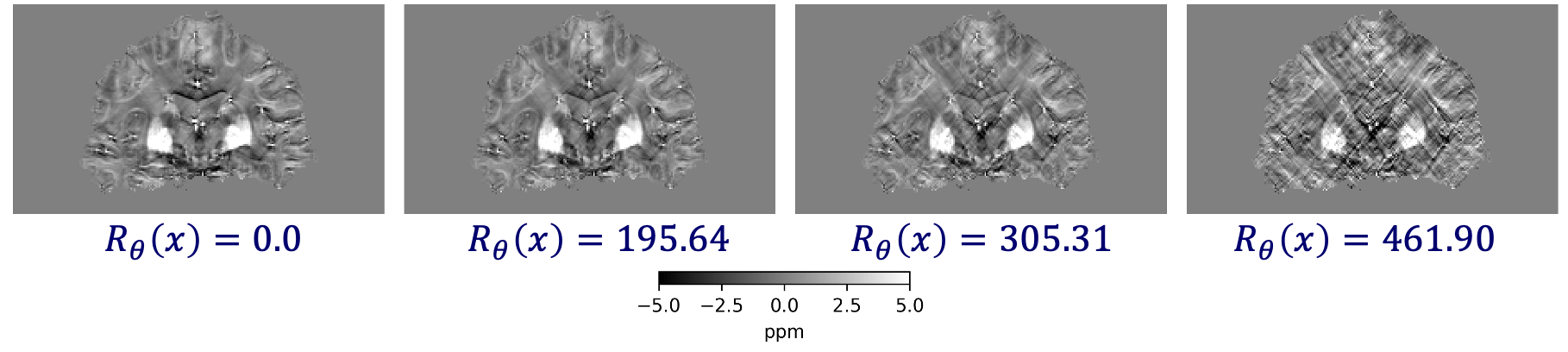
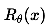
\(R_\theta(x) = 0.0\)
\(R_\theta(x) = 127.37\)
\(R_\theta(x) = 274.13\)
\(R_\theta(x) = 290.45\)
Understanding the learned model provides new insights:
inverse problems
Take-home message 1
- Learned Proximal Networks (LPNs) provide data-dependent proximal operators
- Allow characterization of the learned priors.
inverse problems
uncertainty quantification
model-agnostic interpretability
robustness
generalization
policy & regulation
Demographic fairness
hardware & protocol optimization
data-driven imaging
automatic analysis and rec.
societal implications
Problems in trustworthy biomedical imaging
Demographic fairness
Inputs (features): \(X\in\mathcal X \subset \mathbb R^d\)
Responses (labels): \(Y\in\mathcal Y = \{0,1\}\)
Sensitive attributes \(Z \in \mathcal Z \subseteq \mathbb R^k \) (sex, race, age, etc)
\((X,Y,Z) \sim \mathcal D\)
Eg: \(Z_1: \) biological sex, \(X_1: \) BMI, then
\( g(Z,X) = \boldsymbol{1}\{Z_1 = 1 \land X_1 > 35 \}: \) women with BMI > 35
Goal: ensure that \(f\) is fair w.r.t groups \(g \in \mathcal G\)
Demographic fairness
Group memberships \( \mathcal G = \{ g:\mathcal X \times \mathcal Z \to \{0,1\} \} \)
Predictor \( f(X) : \mathcal X \to [0,1]\) (e.g. likelihood of X having disease Y)
-
Group/Associative Fairness
Predictors should not have very different (error) rates among groups
[Calders et al, '09][Zliobaite, '15][Hardt et al, '16]
-
Individual Fairness
Similar individuals/patients should have similar outputs
[Dwork et al, '12][Fleisher, '21][Petersen et al, '21]
-
Causal Fairness
Predictors should be fair in a counter-factual world
[Nabi & Shpitser, '18][Nabi et al, '19][Plecko & Bareinboim, '22]
-
Multiaccuracy/Multicalibration
Predictors should be approximately unbiased/calibrated for every group
[Kim et al, '20][Hebert-Johnson et al, '18][Globus-Harris et at, 22]
Demographic fairness
-
Multiaccuracy/Multicalibration
Predictors should be approximately unbiased/calibrated for every group
[Kim et al, '20][Hebert-Johnson et al, '18][Globus-Harris et at, 22]
Demographic fairness
Observation 1:
measuring (& correcting) for MA/MC requires samples over \((X,Y,Z)\)
Definition: \(\text{MA} (f,g) = \big| \mathbb E [ g(X,Z) (f(X) - Y) ] \big| \)
\(f\) is \((\mathcal G,\alpha)\)-multiaccurate if \( \max_{g\in\mathcal G} \text{MA}(f,g) \leq \alpha \)
Definition: \(\text{MC} (f,g) = \mathbb E\left[ \big| \mathbb E [ g(X,Z) (f(X) - Y) | f(X) = v] \big| \right] \)
\(f\) is \((\mathcal G,\alpha)\)-multicalibrated if \( \max_{g\in\mathcal G} \text{MC}(f,g) \leq \alpha \)
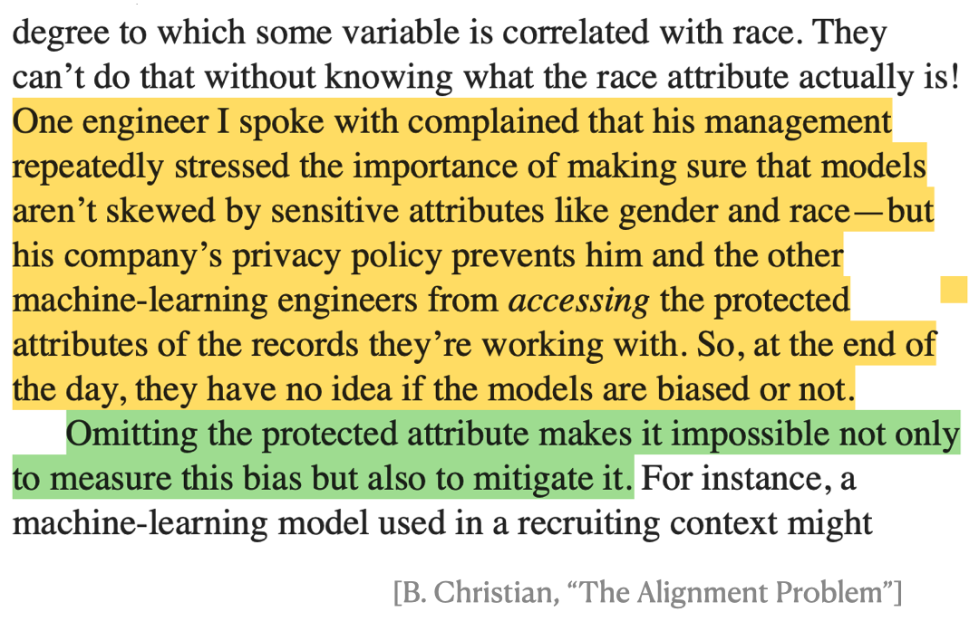
Observation 2: That's not always possible...

Observation 2: That's not always possible...
sex and race attributes missing
- We might want to conceal \(Z\) on purpose, or might need to
We observe samples over \((X,Y)\) to obtain \(\hat Y = f(X)\) for \(Y\)
Fairness in partially observed regimes
\( \text{MSE}(f) = \mathbb E [(Y-f(X))^2 ] \)
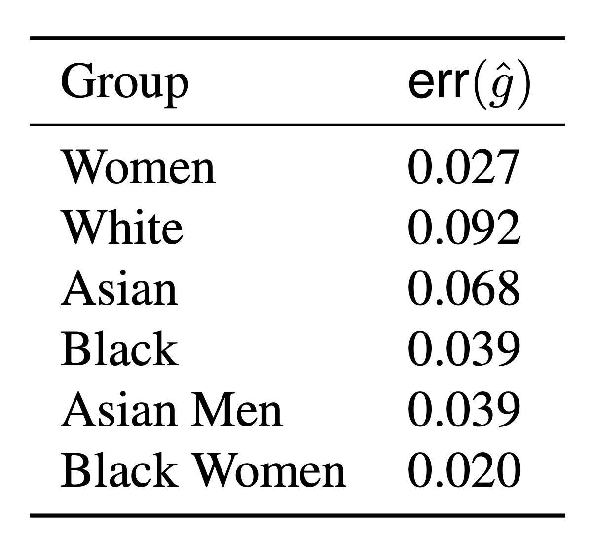
A developer provides us with proxies \( \color{Red} \hat{g} : \mathcal X \to \{0,1\} \)
\( \text{err}(\hat g) = \mathbb P [({\color{Red}\hat g(X)} \neq {\color{blue}g(X,Z)} ] \)
Question 2
Can we (how) use \(\hat g\) to measure (and correct) \( (\mathcal G,\alpha)\)-MA/MC?
[Awasti et al, '21][Kallus et al, '22][Zhu et al, '23][Bharti et al, '24]
Fairness in partially observed regimes
Theorem [Bharti, Clemens-Sewall, Yi, S.]
With access to \((X,Y)\sim \mathcal D_{\mathcal{XY}}\), proxies \( \hat{\mathcal G}\) and predictor \(f\)
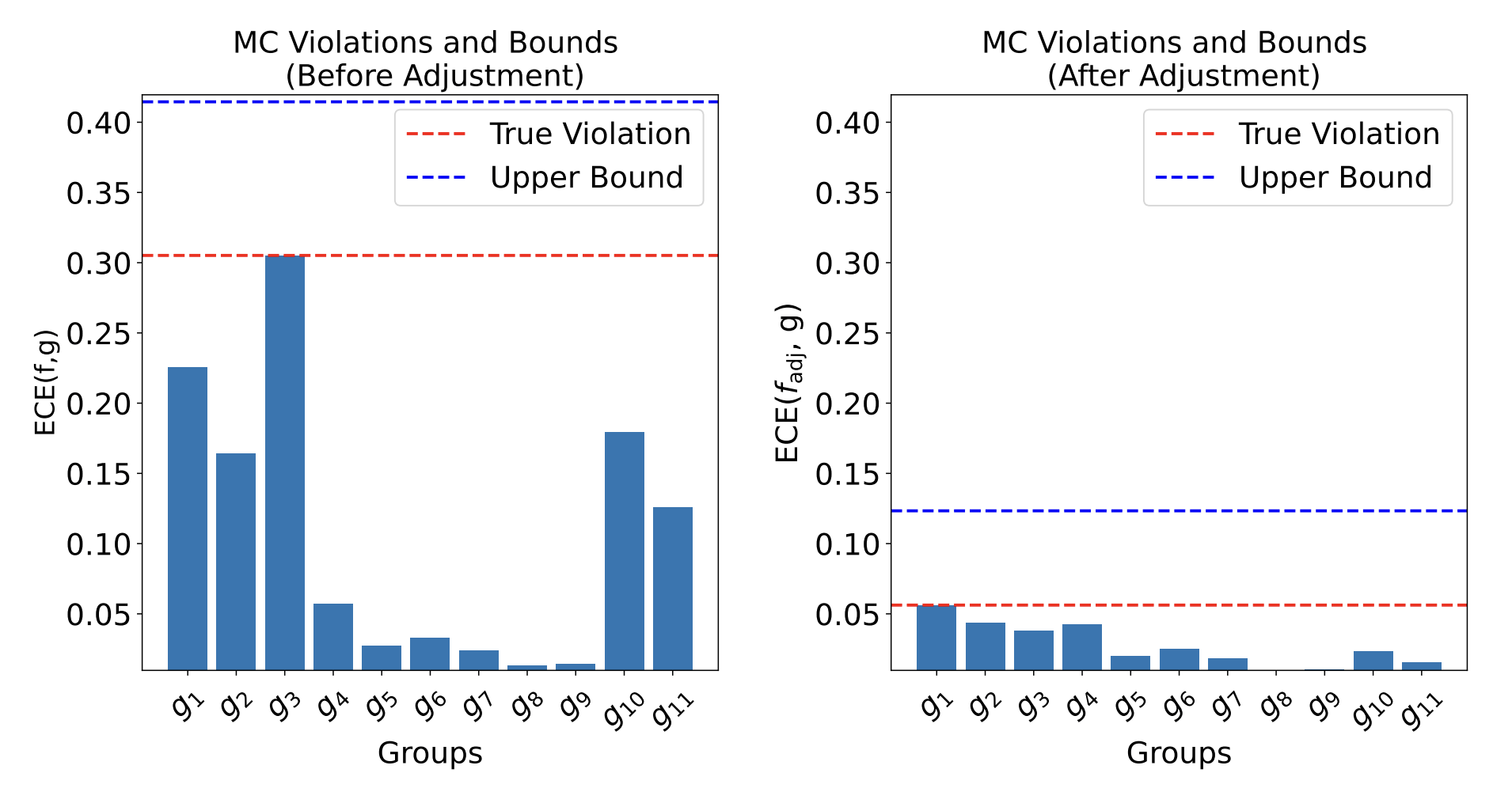
\[ \max_{\color{Blue}g\in\mathcal G} MC(f,{\color{blue}g}) \leq \max_{\color{red}\hat g\in \hat{\mathcal{G}} } B(f,{\color{red}\hat g}) + MC(f,{\color{red}\hat g}) \]
with \(B(f,\hat g) = \min \left( \text{err}(\hat g), \sqrt{MSE(f)\cdot \text{err}(\hat g)} \right) \)
- Practical/computable upper bounds \(\)
- Multicalibrating w.r.t \(\hat{\mathcal G}\) provably improves upper bound
[Gopalan et al. (2022)][Roth (2022)]
Fairness in partially observed regimes

CheXpert: Predicting abnormal findings in chest X-rays
(not accessing race or biological sex)
\(f(X): \) likelihood of \(X\) having \(\texttt{pleural effusion}\)
Demographic fairness
Take-home message 2
- Proxies can be very useful in certifying max. fairness violations
- Can allow for simple post-processing corrections
inverse problems
uncertainty quantification
model-agnostic interpretability
robustness
generalization
policy & regulation
Demographic fairness
hardware & protocol optimization
data-driven imaging
automatic analysis and rec.
societal implications
Problems in trustworthy biomedical imaging
\((X,Y) \in \mathcal X \times \mathcal Y\)
\((X,Y) \sim P_{X,Y}\)
\(\hat{Y} = f(X) : \mathcal X \to \mathcal Y\)
Setting:

-
What features are important for this prediction?
-
What does importance mean, exactly?
model-agnostic interpretability
Is the presence of \(\color{Blue}\texttt{edema}\) important for \(\hat Y = \text{lung opacity}\)?
How can we explain black-box predictors with semantic features?
Is the presence of \(\color{magenta}\texttt{devices}\) important for \(\hat Y = \texttt{lung opacity}\), given that there is \(\color{blue}\texttt{edema}\) in the image?
model-agnostic interpretability
lung opacity
cardiomegaly
fracture
no findding
Post-hoc Interpretability Methods
Interpretable by
construction
Is the presence of \(\color{Blue}\texttt{edema}\) important for \(\hat Y = \text{lung opacity}\)?
How can we explain black-box predictors with semantic features?
Is the presence of \(\color{magenta}\texttt{devices}\) important for \(\hat Y = \texttt{lung opacity}\), given that there is \(\color{blue}\texttt{edema}\) in the image?
model-agnostic interpretability
lung opacity
cardiomegaly
fracture
no findding
Interpretable by
construction
Post-hoc Interpretability Methods
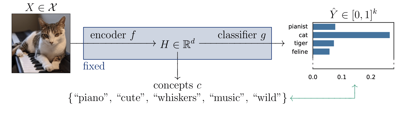
Semantic Interpretability of classifiers
Concept Bank: \(C = [c_1, c_2, \dots, c_m] \in \mathbb R^{d\times m}\)
Embeddings: \(H = f(X) \in \mathbb R^d\)
Semantics: \(Z = C^\top H \in R^m\)
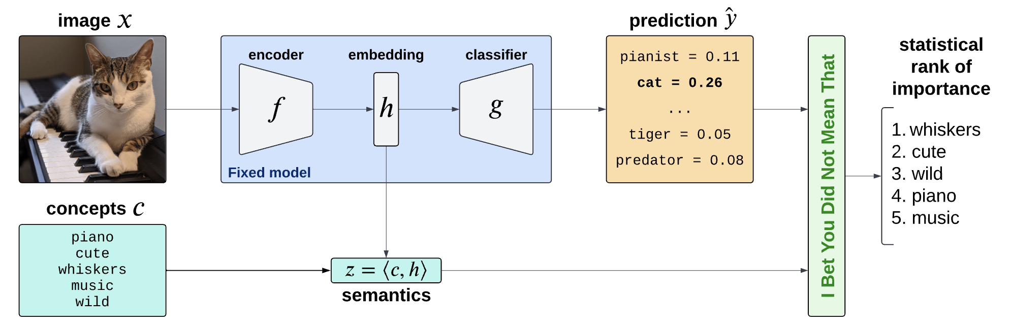
Semantic Interpretability of classifiers
Question 3 (last!)
How can we provide (local) notions of importance that allow for (efficient) statistical testing with valid guarantees (Type 1 error/FDR control)
Concept Bank: \(C = [c_1, c_2, \dots, c_m] \in \mathbb R^{d\times m}\)
Concept Activation Vectors
(Kim et al, 2018)
\(c_\text{cute}\)
Semantic Interpretability of classifiers
Vision-language models
(CLIP, BLIP, etc... )
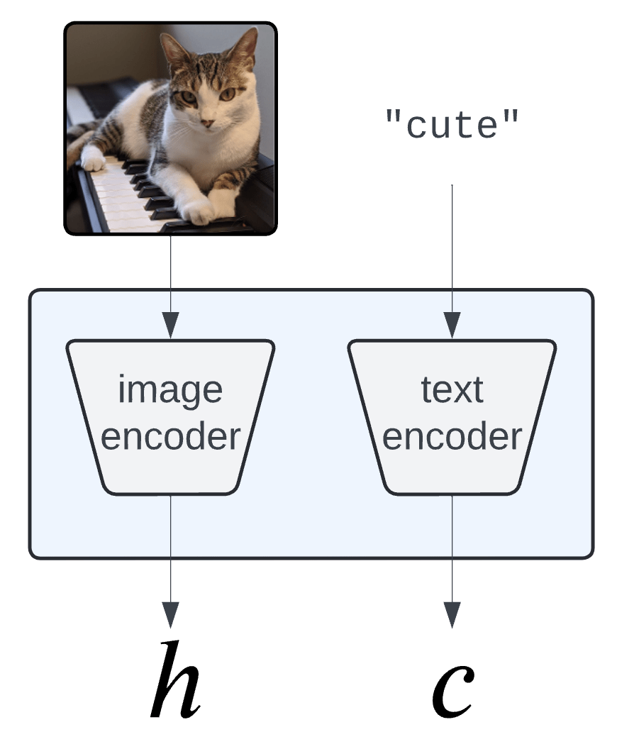
Concept Bank: \(C = [c_1, c_2, \dots, c_m] \in \mathbb R^{d\times m}\)
Semantic Interpretability of classifiers
Vision-language models
(training)
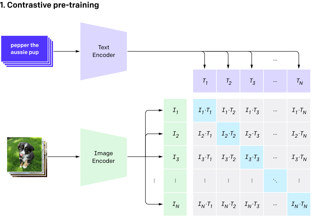
[Radford et al, 2021]
Semantic Interpretability of classifiers
[Bhalla et al, "Splice", 2024]
Concept Bottleneck Models (CMBs)
[Koh et al '20, Yang et al '23, Yuan et al '22 ]
- Need to engineer a (large) concept bank
- Performance hit w.r.t. original predictor
\(\tilde{Y} = \hat w^\top Z\)
\(\hat w_j\) is the importance of the \(j^{th}\) concept
Precise notions of semantic importance
\(C = \{\text{``cute''}, \text{``whiskers''}, \dots \}\)
Global Importance
\(H^G_{0,j} : \hat{Y} \perp\!\!\!\perp Z_j \)
Global Conditional Importance
\(H^{GC}_{0,j} : \hat{Y} \perp\!\!\!\perp Z_j | Z_{-j}\)
Precise notions of semantic importance
Global Importance
\(C = \{\text{``cute''}, \text{``whiskers''}, \dots \}\)
\(H^G_{0,j} : g(f(X)) \perp\!\!\!\perp c_j^\top f(X) \)
Global Conditional Importance
\(H^{GC}_{0,j} : g(f(X)) \perp\!\!\!\perp c_j^\top f(X) | C_{-j}^\top f(X)\)
\(H^G_{0,j} : \hat{Y} \perp\!\!\!\perp Z_j \)
\(H^{GC}_{0,j} : \hat{Y} \perp\!\!\!\perp Z_j | Z_{-j}\)
Precise notions of semantic importance
"The classifier (its distribution) does not change if we condition
on concepts \(S\) vs on concepts \(S\cup\{j\} \)"
\(C = \{\texttt{cute}, \texttt{whiskers}, \dots \}\)
Local Conditional Importance
\[H^{j,S}_0:~ g({\tilde H_{S \cup \{j\}}}) \overset{d}{=} g(\tilde H_S), \qquad \tilde H_S \sim P_{H|Z_S = C_S^\top f(x)} \]
Tightly related to Shapley values
[Teneggi et al, The Shapley Value Meets Conditional Independence Testing, 2023]
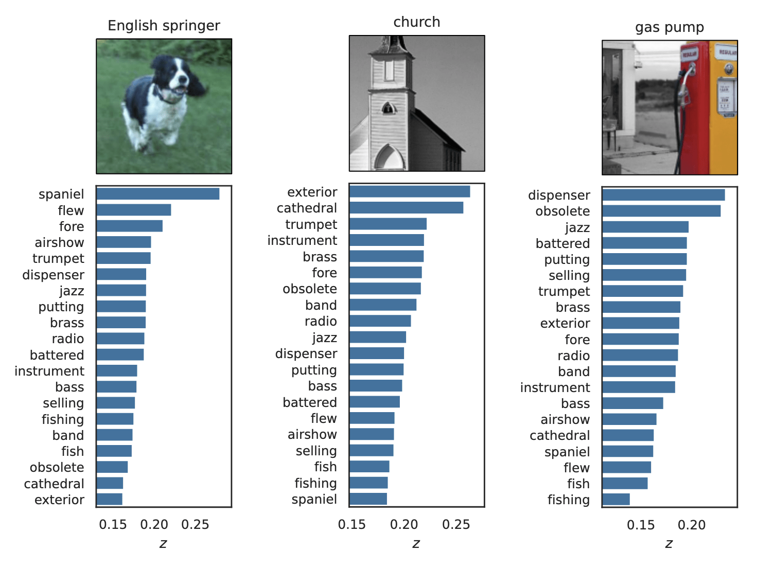
Precise notions of semantic importance
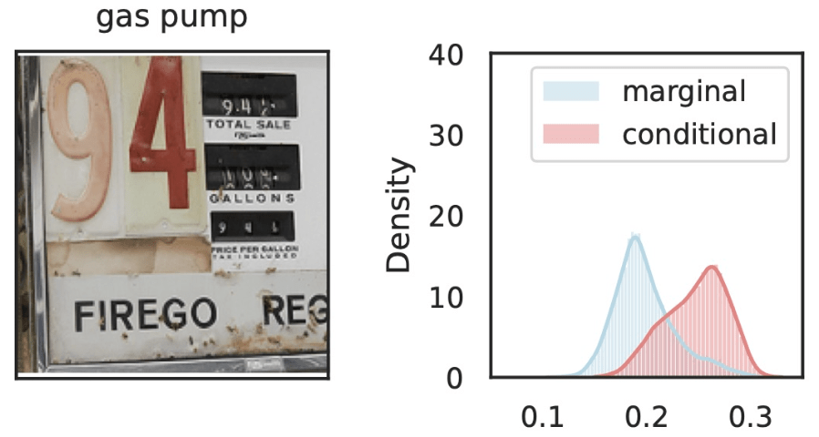

\(\hat{Y}_\text{gas pump}\)
\(Z_S\cup Z_{j}\)
\(Z_{S}\)
\(Z_j=\)
Local Conditional Importance
\[H^{j,S}_0:~ g({\tilde H_{S \cup \{j\}}}) \overset{d}{=} g(\tilde H_S), \qquad \tilde H_S \sim P_{H|Z_S = C_S^\top f(x)} \]
\(\tilde{Z}_S = [z_\text{text}, z_\text{old}, Z_\text{dispenser}, Z_\text{trumpet}, Z_\text{fire}, \dots ] \)
\(S\)

\(\tilde{Z}_{S\cup j} = [z_\text{text}, z_\text{old}, z_\text{dispenser}, Z_\text{trumpet}, Z_\text{Fire}, \dots ] \)
\(S\)
\(j\)
Precise notions of semantic importance
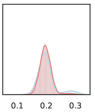

\(\hat{Y}_\text{gas pump}\)
\(\hat{Y}_\text{gas pump}\)
\(Z_S\cup Z_{j}\)
\(Z_{S}\)
\(Z_S\cup Z_{j}\)
\(Z_{S}\)
Local Conditional Importance
\(Z_j=\)
\(Z_j=\)
\[H^{j,S}_0:~ g({\tilde H_{S \cup \{j\}}}) \overset{d}{=} g(\tilde H_S), \qquad \tilde H_S \sim P_{H|Z_S = C_S^\top f(x)} \]
\(\tilde{Z}_S = [z_\text{text}, z_\text{old}, Z_\text{dispenser}, Z_\text{trumpet}, Z_\text{fire}, \dots ] \)
\(\tilde{Z}_{S\cup j} = [z_\text{text}, z_\text{old}, Z_\text{dispenser}, z_\text{trumpet}, Z_\text{Fire}, \dots ] \)
\(S\)
\(S\)
\(j\)
Testing by betting
\(H^G_{0,j} : \hat{Y} \perp\!\!\!\perp Z_j \iff P_{\hat{Y},Z_j} = P_{\hat{Y}} \times P_{Z_j}\)
Testing importance via two-sample tests
\(H^{GC}_{0,j} : \hat{Y} \perp\!\!\!\perp Z_j | Z_{-j} \iff P_{\hat{Y}Z_jZ_{-j}} = P_{\hat{Y}\tilde{Z}_j{Z_{-j}}}\)
\(\tilde{Z_j} \sim P_{Z_j|Z_{-j}}\)
[Shaer et al, 2023]
[Teneggi et al, 2023]
\[H^{j,S}_0:~ g({\tilde H_{S \cup \{j\}}}) \overset{d}{=} g(\tilde H_S), \qquad \tilde H_S \sim P_{H|Z_S = C_S^\top f(x)} \]
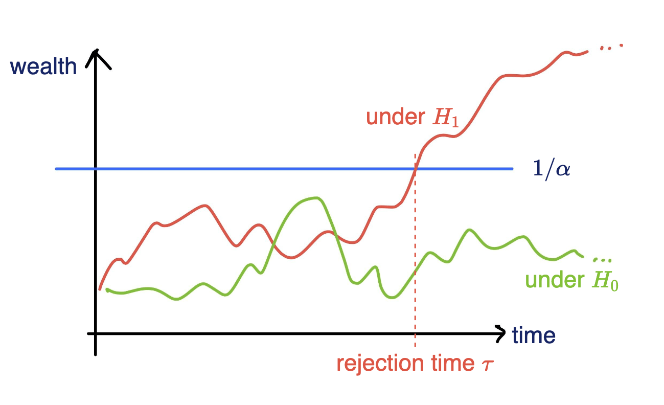
Testing by betting
Goal: Test a null hypothesis \(H_0\) at significance level \(\alpha\)
Standard testing by p-values
Collect data, then test, and reject if \(p \leq \alpha\)
[Grünwald 2019, Shafer 2021, Shaer et al. 2023, Shekhar and Ramdas 2023. Podkopaev et al., 2023]
Testing by betting
Goal: Test a null hypothesis \(H_0\) at significance level \(\alpha\)
Online testing by e-values
Any-time valid inference, track and reject when \(e\geq 1/\alpha\)
- Consider a wealth process
\(K_0 = 1;\)
\(\text{for}~ t = 1, \dots \\ \quad K_t = K_{t-1}(1+\kappa_t v_t)\)
Fair game (test martingale): \(~~\mathbb E_{H_0}[\kappa_t | \text{Everything seen}_{t-1}] = 0\)
\(v_t \in (0,1):\) betting fraction
\(\kappa_t \in [-1,1]\) payoff
[Grünwald 2019, Shafer 2021, Shaer et al. 2023, Shekhar and Ramdas 2023. Podkopaev et al., 2023]
\(\mathbb P_{H_0}[\exists t \in \mathbb N: K_t \leq 1/\alpha]\leq \alpha\)
Data efficient
Rank induced by rejection time
Testing by betting
Goal: Test a null hypothesis \(H_0\) at significance level \(\alpha\)
Online testing by e-values
Any-time valid inference, track and reject when \(e\geq 1/\alpha\)
- Consider a wealth process
\(K_0 = 1;\)
\(\text{for}~ t = 1, \dots \\ \quad K_t = K_{t-1}(1+\kappa_t v_t)\)
Fair game (test martingale): \(~~\mathbb E_{H_0}[\kappa_t | \text{Everything seen}_{t-1}] = 0\)
\(v_t \in (0,1):\) betting fraction
\(\kappa_t \in [-1,1]\) payoff
[Grünwald 2019, Shafer 2021, Shaer et al. 2023, Shekhar and Ramdas 2023. Podkopaev et al., 2023]
Data efficient
Rank induced by rejection time
\(\mathbb P_{H_0}[\exists t \in \mathbb N: K_t \leq 1/\alpha]\leq \alpha\)
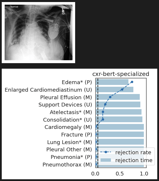
Testing by betting via SKIT (Podkopaev et al., 2023)
Online testing by e-values
\(v_t \in (0,1):\) betting fraction
\(H_0: ~ P = Q\)
\(\kappa_t = \text{tanh}({\color{teal}\rho(X_t)} - {\color{teal}\rho(Y_t)})\)
Payoff function
\({\color{black}\text{MMD}(P,Q)} : \text{ Maximum Mean Discrepancy}\)
\({\color{teal}\rho} = \underset{\rho\in \mathcal R:\|\rho\|_\mathcal R\leq 1}{\arg\sup} ~\mathbb E_P [\rho(X)] - \mathbb E_Q[\rho(Y)]\)
\( K_t = K_{t-1}(1+\kappa_t v_t)\)
Data efficient
Rank induced by rejection time
\(X_t \sim P, Y_t \sim Q\)
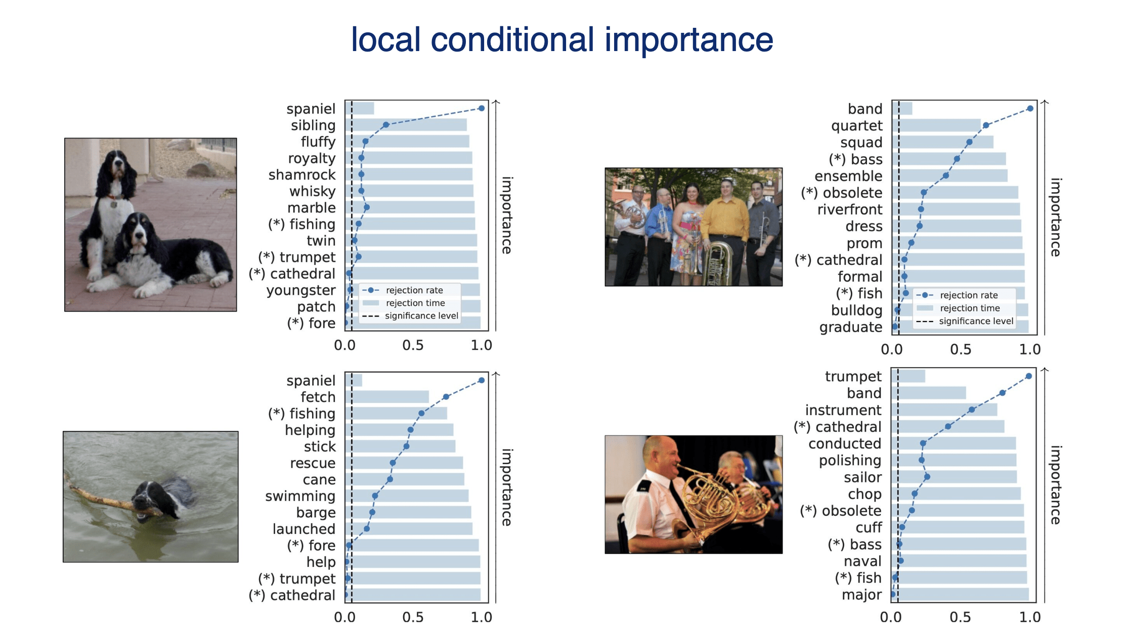
Results: Local Testing
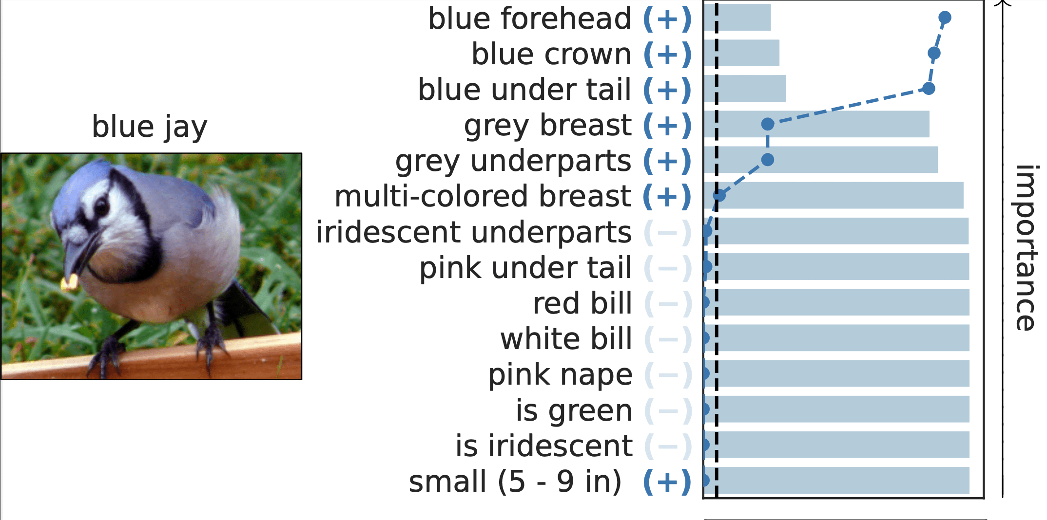
Important Semantic Concepts
(Reject \(H_0\))

Unimportant Semantic Concepts
(Fail to reject)
- Type 1 error control
- False discovery rate control
rejection time
rejection rate
0.0
1.0
Results: Local Testing

CheXpert: validating BiomedVLP
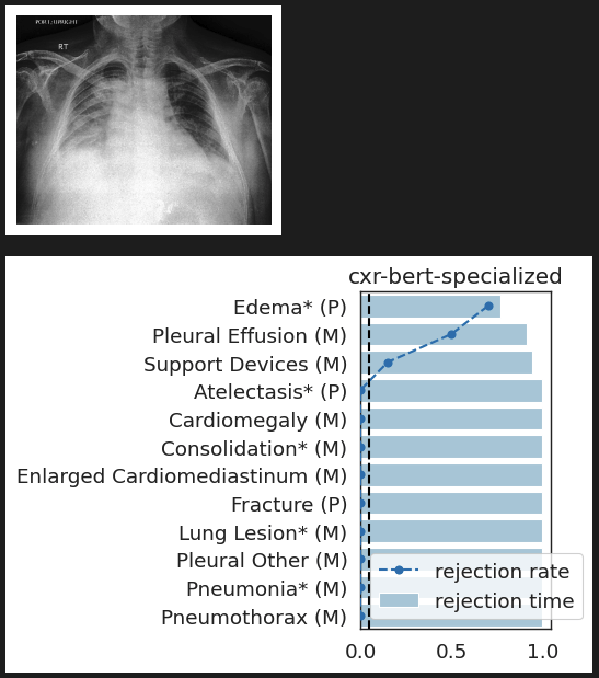
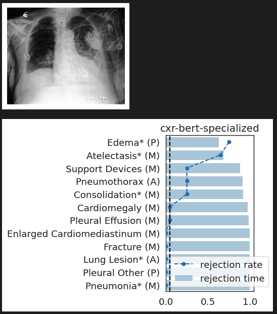
What concepts does BiomedVLP find important to predict ?
lung opacityCheXpert: validating BiomedVLP
What concepts does BiomedVLP find important to predict ?
lung opacityTake-home message 3
- Model-agnostic interpretability can be posed as local hypothesis tests
- Online efficient testing procedures for statistical control
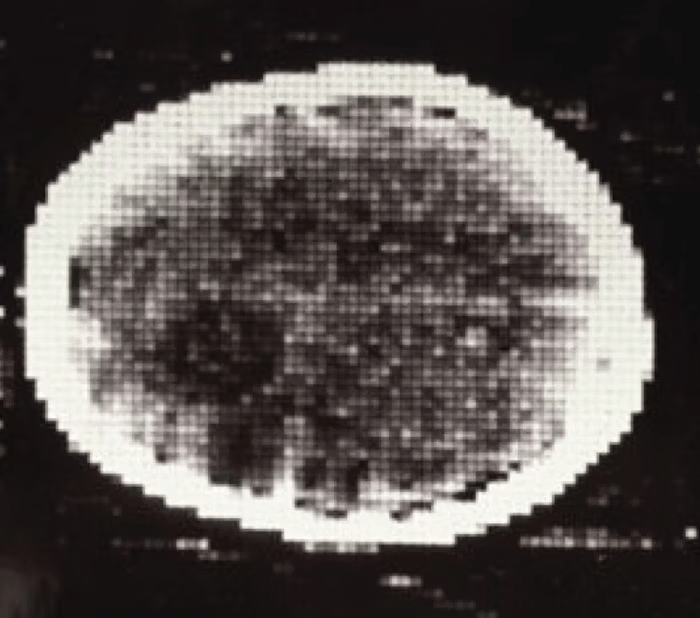
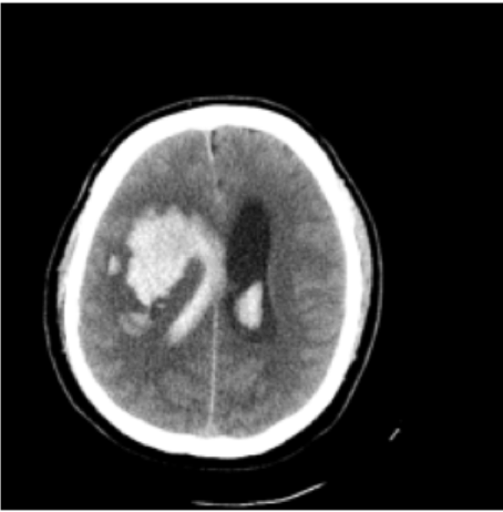
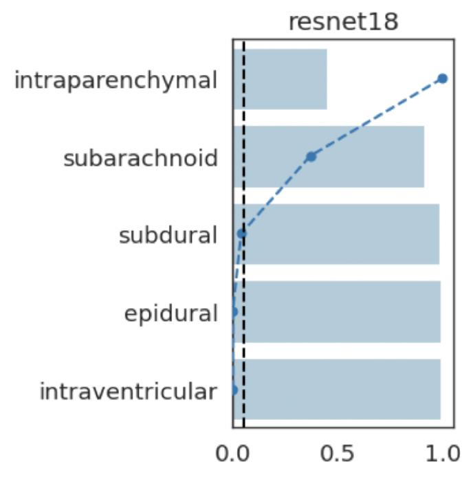
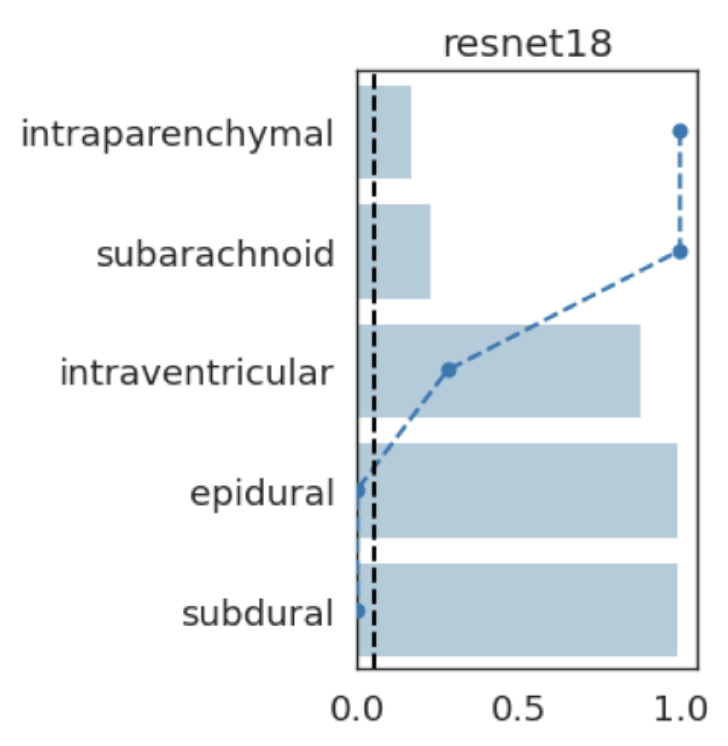
Results: RSNA Brain CT Hemorrhage
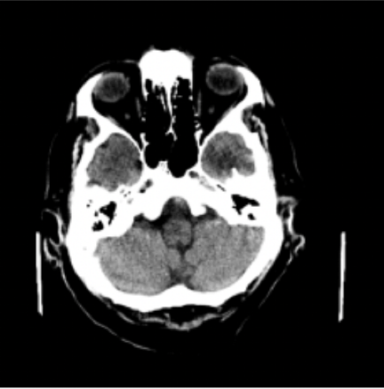
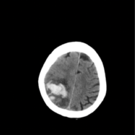
Hemorrhage
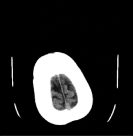
No Hemorrhage
Hemorrhage
Hemorrhage
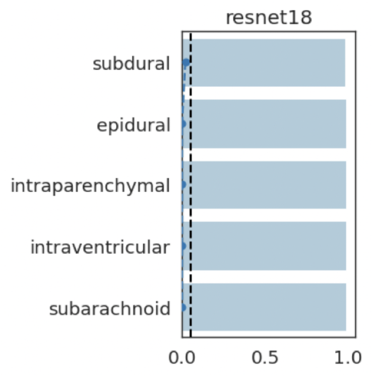
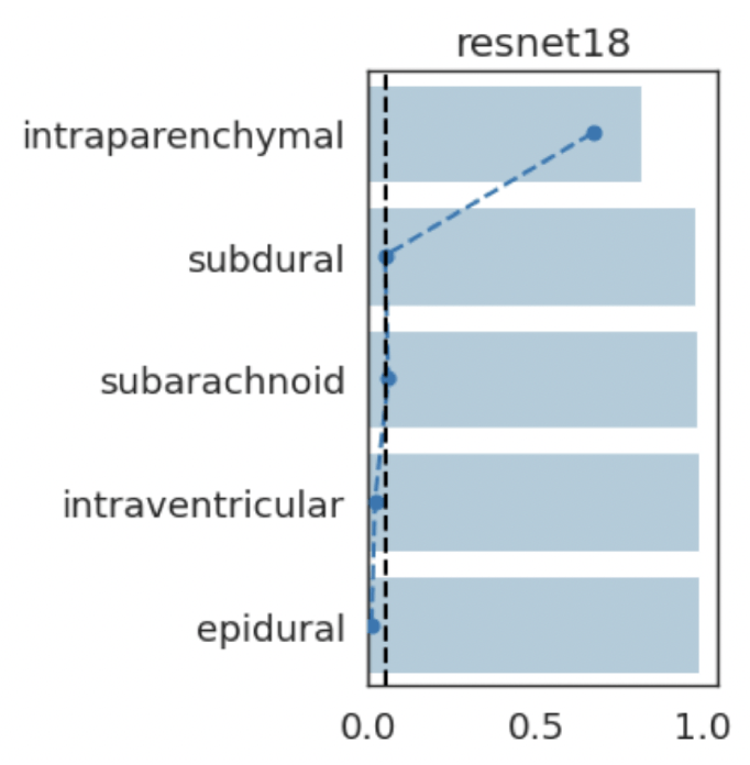
intraparenchymal
subdural
subarachnoid
intraventricular
epidural
intraparenchymal
subarachnoid
intraventricular
epidural
subdural
intraparenchymal
subarachnoid
subdural
epidural
intraventricular
intraparenchymal
subarachnoid
intraventricular
epidural
subdural
(+)
(-)
(-)
(-)
(-)
(+)
(-)
(+)
(-)
(-)
(+)
(+)
(-)
(-)
(-)
(-)
(-)
(-)
(-)
(-)
Take-home message 3
- Model-agnostic interpretability can be posed as local hypothesis tests
- Online efficient testing procedures for statistical control
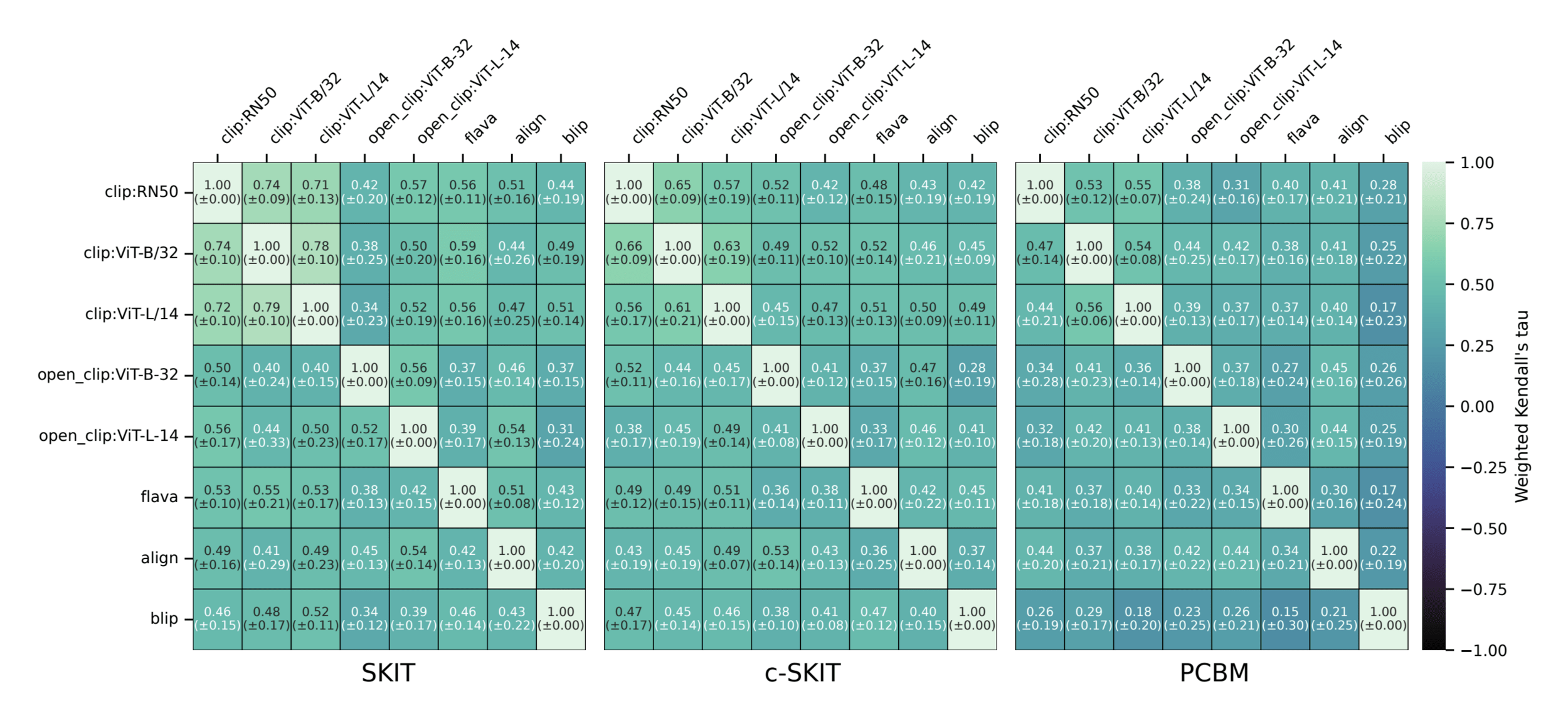
Results: Imagenette
Semantic comparison of vision-language models
inverse problems
uncertainty quantification
model-agnostic interpretability
robustness
generalization
policy & regulation
Demographic fairness
hardware & protocol optimization
data-driven imaging
automatic analysis and rec.
societal implications
Problems in trustworthy biomedical imaging
model-agnostic interpretability
uncertainty quantification
policy & regulation
hardware & protocol optimization
inverse problems
Demographic fairness
robustness
generalization
[Bharti et al, Neurips '23 ]
[Bharti et al, arXiv '25 ]
[Sulam et al, Neurips '20 ]
[Muthukumar et al, COLT '23 ]
[Pal et al, Neurips '24]
[Muthukumar et al, SIMODS '23]
[Pal et al, TMLR '24]
[Teneggi et al, TMLR '22]
[Teneggi et al, TPAMI '22]
[Teneggi et al, Neurips '24]
[Bharti et al, CPAL '25]
[Teneggi et al, ICML '23]
[Teneggi et al, arXiv '25]
[Muthukumar et al, CVPR '25]
[Lai et al, MICCAI '20]
[Fang et al, MIA '20]
[Xu et al, Nat.Met'20]
[Fang et al, ICLR '24]
data-driven imaging
automatic analysis and rec.
societal implications
[Wang et al, CPAL '25]
[Wang et al, Patterns '25]
uncertainty quantification
policy & regulation
hardware & protocol optimization
robustness
generalization
data-driven imaging
automatic analysis and rec.
societal implications
inverse problems
Societal Constraints
model-agnostic interpretability
Formal frameworks for interpretability for decision making (in medical imaging)
Understanding social implications of algorithms in the wild
Efficient and robust diffusion models
uncertainty quantification
robustness
generalization
uncertainty quantification
Many more open questions...


Thank you for hosting me

Learned Proximal Networks
Example 2: a prior for CT
Learned Proximal Networks
Example 2: a prior for CT
Learned Proximal Networks
Example 2: a prior for CT
Learned Proximal Networks
Example 2: a prior for CT
Learned Proximal Networks

\(R(\tilde{x})\)
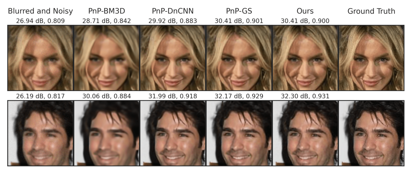
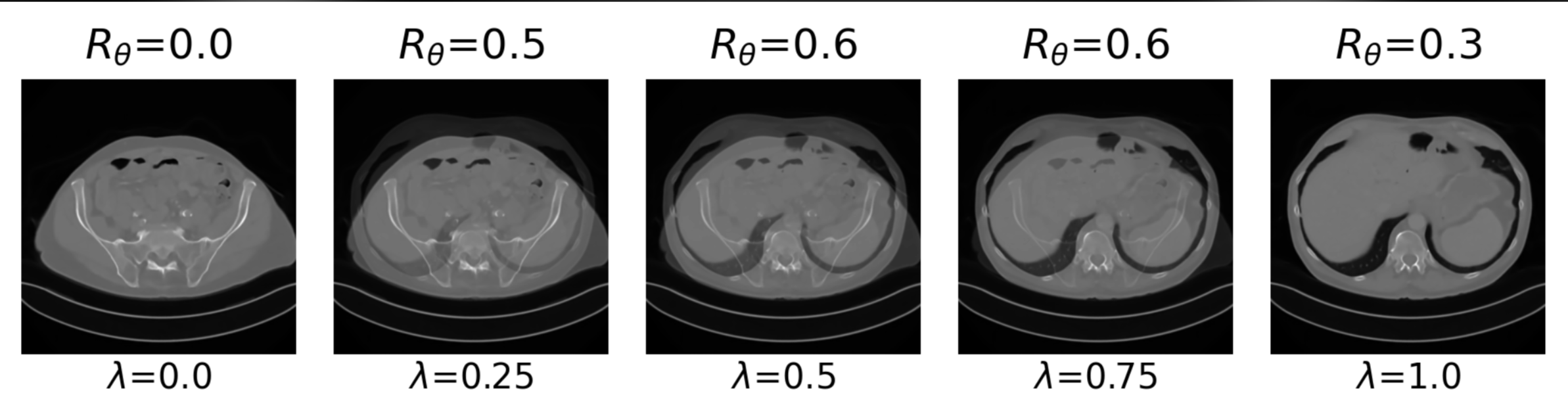
Example 2: priors for images
Learned Proximal Networks
Example 2: priors for images
Learned Proximal Networks
via
Convergence Guarantees
Theorem (PGD with Learned Proximal Networks)
Let \(f_\theta = \text{prox}_{\hat{R}} {\color{grey}\text{ with } \alpha>0}, \text{ and } 0<\eta<1/\sigma_{\max}(A) \) with smooth activations
(Analogous results hold for ADMM)
Learned Proximal Networks
Convergence guarantees for PnP

in a box
Denoiser
diffusion
Measurements
\[y = Ax + \epsilon,~\epsilon \sim \mathcal{N}(0, \sigma^2\mathbb{I})\]
\[\hat{x} = F(y) \sim \mathcal{P}_y\]
Hopefully \(\mathcal{P}_y \approx p(x \mid y)\), but not needed!

Reconstruction
Question 3)
How much uncertainty is there in the samples \(\hat x \sim \mathcal P_y?\)
Question 4)
How far will the samples \(\hat x \sim \mathcal P_y\) be from the true \(x\)?
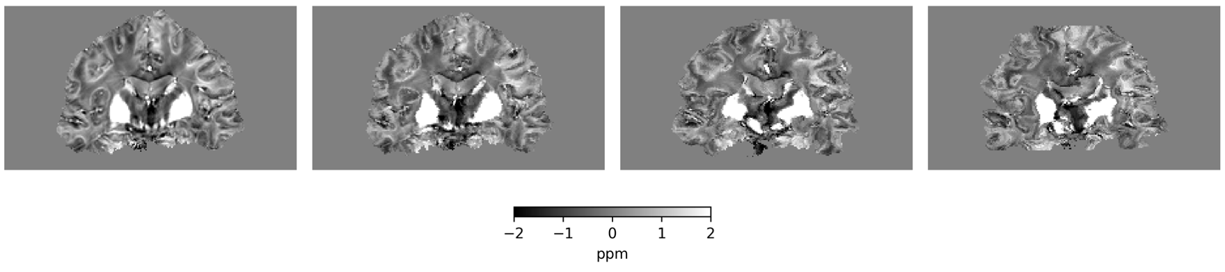
Conformal guarantees for diffusion models
Lemma
Given \(m\) samples from \(\mathcal P_y\), let
\[\mathcal{I}(y)_j = \left[ Q_{y_j}\left(\frac{\lfloor(m+1)\alpha/2\rfloor}{m}\right), Q_{y_j}\left(\frac{\lceil(m+1)(1-\alpha/2)\rceil}{m}\right)\right]\]
Then \(\mathcal I(y)\) provides entriwise coverage for a new sample \(\hat x \sim \mathcal P_y\), i.e.
\[\mathbb{P}\left[\hat{x}_j \in \mathcal{I}(y)_j\right] \geq 1 - \alpha\]
\(0\)
\(1\)
low: \( l(y) \)
\(\mathcal{I}(y)\)
up: \( u(y) \)
Question 3)
How much uncertainty is there in the samples \(\hat x \sim \mathcal P_y?\)
(distribution free)
cf [Feldman, Bates, Romano, 2023]

\(y\)
lower
upper
intervals
\(|\mathcal I(y)_j|\)
Conformal guarantees for diffusion models
\(0\)
\(1\)
ground-truth is
contained
\(\mathcal{I}(y_j)\)
\(x_j\)
Conformal guarantees for diffusion models
Question 4)
How far will the samples \(\hat x \sim \mathcal P_y\) be from the true \(x\)?
Conformal guarantees for diffusion models
[Angelopoulos et al, 2022]
[Angelopoulos et al, 2022]
Risk Controlling Prediction Set
For risk level \(\epsilon\), failure probability \(\delta\), \(\mathcal{I}(y_j) \) is a RCPS if
\[\mathbb{P}\left[\mathbb{E}\left[\text{fraction of pixels not in intervals}\right] \leq \epsilon\right] \geq 1 - \delta\]
[Angelopoulos et al, 2022]
Question 4)
How far will the samples \(\hat x \sim \mathcal P_y\) be from the true \(x\)?
\(0\)
\(1\)
ground-truth is
contained
\(\mathcal{I}(y_j)\)
\(x_j\)
Conformal guarantees for diffusion models
[Angelopoulos et al, 2022]
ground-truth is
contained
\(0\)
\(1\)
\(\mathcal{I}(y_j)\)
\(\lambda\)
\(x_j\)
Procedure:
\[\hat{\lambda} = \inf\{\lambda \in \mathbb{R}:~ \hat{\text{risk}}_{(\mathcal S_{cal})} \leq \epsilon,~\forall \lambda' \geq \lambda \}\]
[Angelopoulos et al, 2022]
single \(\lambda\) for all \(\mathcal I(y_j)\)!
Risk Controlling Prediction Set
For risk level \(\epsilon\), failure probability \(\delta\), \(\mathcal{I}(y_j) \) is a RCPS if
\[\mathbb{P}\left[\mathbb{E}\left[\text{fraction of pixels not in intervals}\right] \leq \epsilon\right] \geq 1 - \delta\]
[Angelopoulos et al, 2022]
Question 4)
How far will the samples \(\hat x \sim \mathcal P_y\) be from the true \(x\)?
\(\mathcal{I}_{\bm{\lambda}}(y)_j = [l_\text{low,j} - \lambda, l_\text{up,j} + \lambda]\)
Conformal guarantees for diffusion models
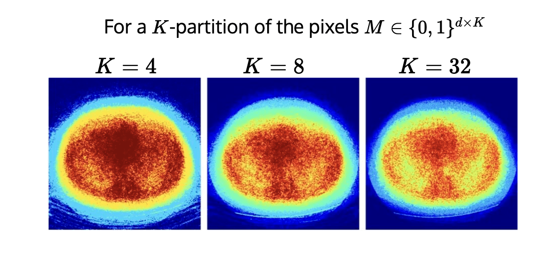
\(K\)-RCPS: High-dimensional Risk Control
\[\tilde{{\lambda}}_K = \underset{\lambda \in \mathbb R^K}{\arg\min}~\sum_{k \in [K]}\lambda_k~\quad \text{s.t. }\quad \mathcal I_{\lambda_j}(y) : \text{RCPS}\]
scalar \(\lambda \in \mathbb{R}\)
vector \(\bm{\lambda} \in \mathbb{R}^d\)
\(\mathcal{I}_{\lambda}(y)_j = [\text{low}_j - \lambda, \text{up}_j + \lambda]\)
\(\mathcal{I}_{\bm{\lambda}}(y)_j = [\text{low}_j - \lambda_j, \text{up}_j + \lambda_j]\)
\(\rightarrow\)
\(\rightarrow\)
Procedure:
1. Find anchor point
\[\tilde{\bm{\lambda}}_K = \underset{\bm{\lambda}}{\arg\min}~\sum_{k \in [K]}\lambda_k~\quad\text{s.t.}~~~\hat{\text{risk}}^+(\bm{\lambda})_{(S_{opt})} \leq \epsilon\]
2. Choose
\[\hat{\beta} = \inf\{\beta \in \mathbb{R}:~\hat{\text{risk}}_{S_{cal}}^+(\tilde{\bm{\lambda}}_K + \beta'\bf{1}) \leq \epsilon,~\forall~ \beta' \geq \beta\}\]
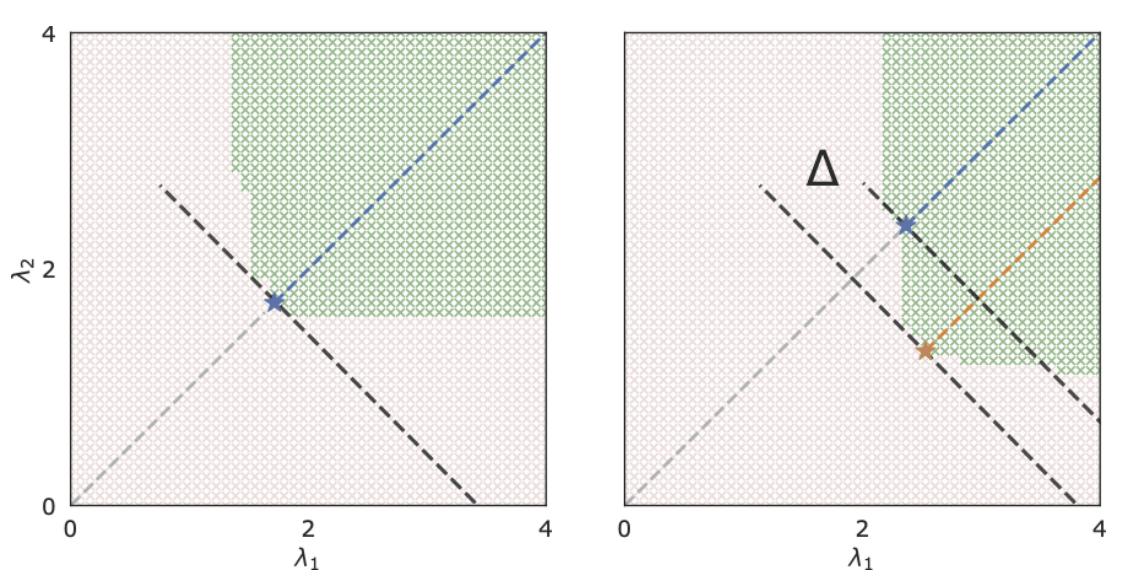
\(\tilde{\bm{\lambda}}_K\)
Conformal guarantees for diffusion models
\(K\)-RCPS: High-dimensional Risk Control
\[\tilde{{\lambda}}_K = \underset{\lambda \in \mathbb R^K}{\arg\min}~\sum_{k \in [K]}\lambda_k~\quad \text{s.t. }\quad \mathcal I_{\lambda_j}(y) : \text{RCPS}\]
scalar \(\lambda \in \mathbb{R}\)
vector \(\bm{\lambda} \in \mathbb{R}^d\)
\(\rightarrow\)
\(\rightarrow\)
Procedure:
1. Find anchor point
\[\tilde{\bm{\lambda}}_K = \underset{\bm{\lambda}}{\arg\min}~\sum_{k \in [K]}\lambda_k~\quad\text{s.t.}~~~\hat{\text{risk}}^+(\bm{\lambda})_{(S_{opt})} \leq \epsilon\]
2. Choose
\[\hat{\beta} = \inf\{\beta \in \mathbb{R}:~\hat{\text{risk}}_{S_{cal}}^+(\tilde{\bm{\lambda}}_K + \beta'\bf{1}) \leq \epsilon,~\forall~ \beta' \geq \beta\}\]
\(\hat{R}^{\gamma}(\bm{\lambda}_{S_{opt}})\leq \epsilon\)
Guarantee: \(\mathcal{I}_{\bm{\lambda}_K,\hat{\beta}}(y)_j \) are \((\epsilon,\delta)\)-RCPS
\(\tilde{\bm{\lambda}}_K\)
\(\mathcal{I}_{\lambda}(y)_j = [\text{low}_j - \lambda, \text{up}_j + \lambda]\)
\(\mathcal{I}_{\bm{\lambda}}(y)_j = [\text{low}_j - \lambda_j, \text{up}_j + \lambda_j]\)

\(\hat{\lambda}_K\)
conformalized uncertainty maps
\(K=4\)
\(K=8\)
\[\mathbb{P}\left[\mathbb{E}\left[\text{fraction of pixels not in intervals}\right] \leq \epsilon\right] \geq 1 - \delta\]
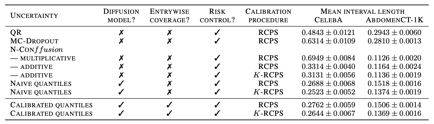
Conformal guarantees for diffusion models
c.f. [Kiyani et al, 2024]
Teneggi, Tivnan, Stayman, S. How to trust your diffusion model: A convex optimization approach to conformal risk control. ICML 2023