
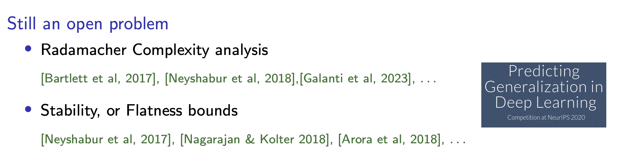
Understanding deep nets
Local Lipschitz functions and learned proximal networks
Jeremias Sulam

SILO Seminar - Nov 2023


Important Open Questions


Important Open Questions
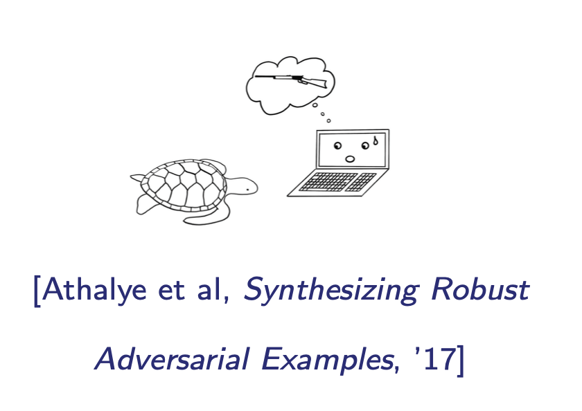
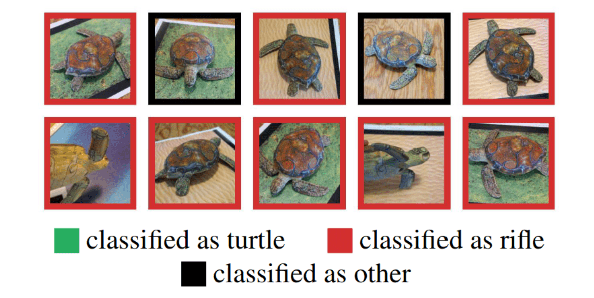
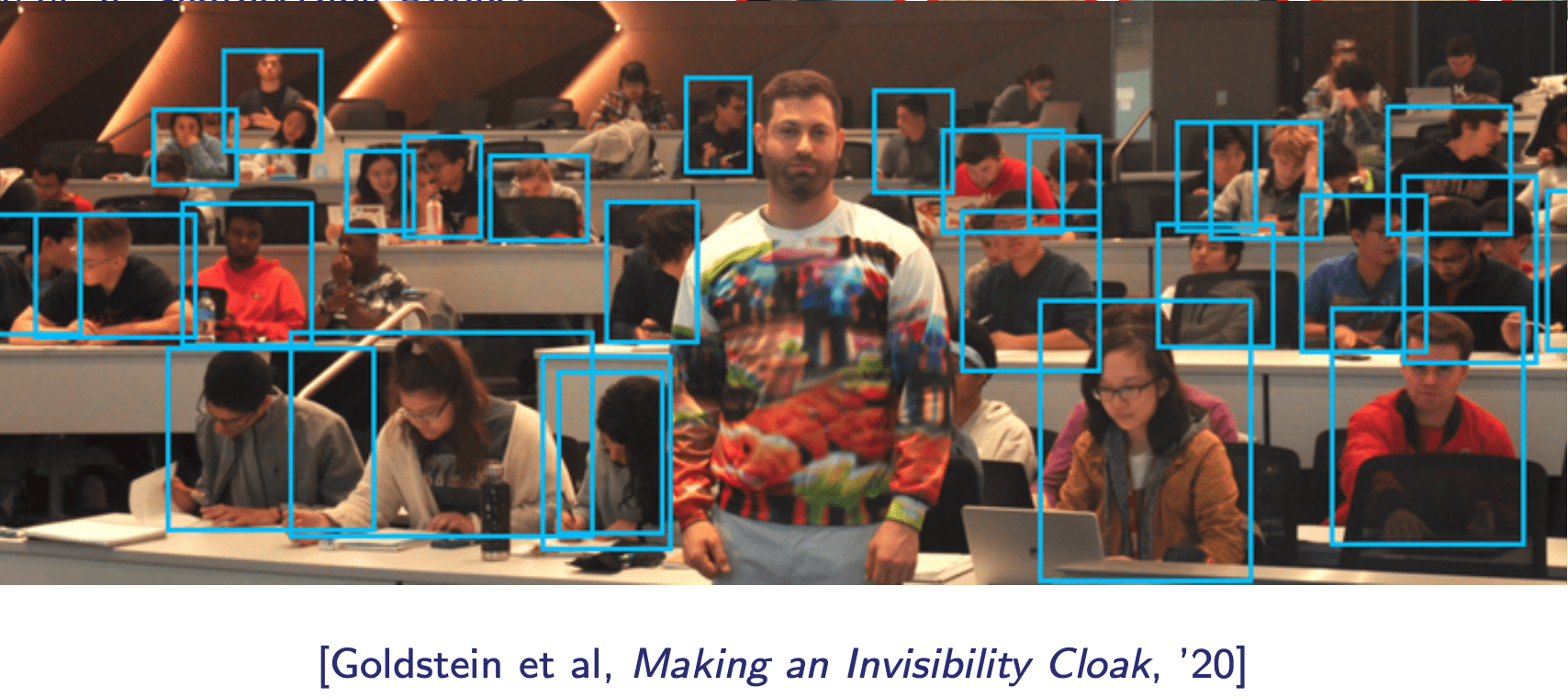
1. Adversarial Attacks
Imperceptible perturbations (to humans) to inputs can compromise ML systems
Important Open Questions

1. Adversarial Attacks
Imperceptible perturbations (to humans) to inputs can compromise ML systems
2. Generalization
Estimate the risk of a model from training samples
1. Adversarial Attacks
Imperceptible perturbations (to humans) to inputs can compromise ML systems
2. Generalization
Estimate the risk of a model from training samples
Important Open Questions
3. Deep models in Inverse Problems
How should standard restoration approaches be adapted to exploit deep learning models?

1. Adversarial Attacks
2. Generalization
Agenda
3. Deep models in Inverse Problems
PART I
Local Sparse Lipschitzness
PART II
Learned Proximal NetworksPART I
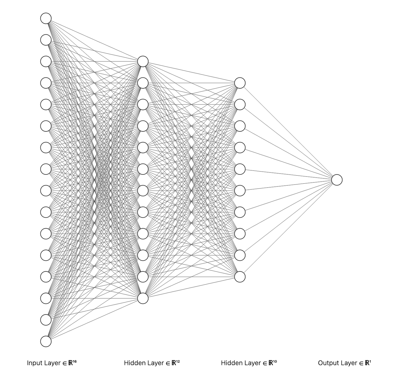
Local Sparse LipschitznessSetting
Hypothesis Class
nonlinear, complex function
Hypothesis Class
Sensitivity
"Complex Deep Nets are locally simple"
"Complex Deep Nets are locally simple"
Today's Agenda


Adversarial Robustness
Generalization
Learning to solve Inverse Problems
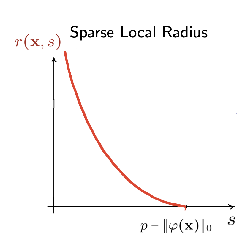
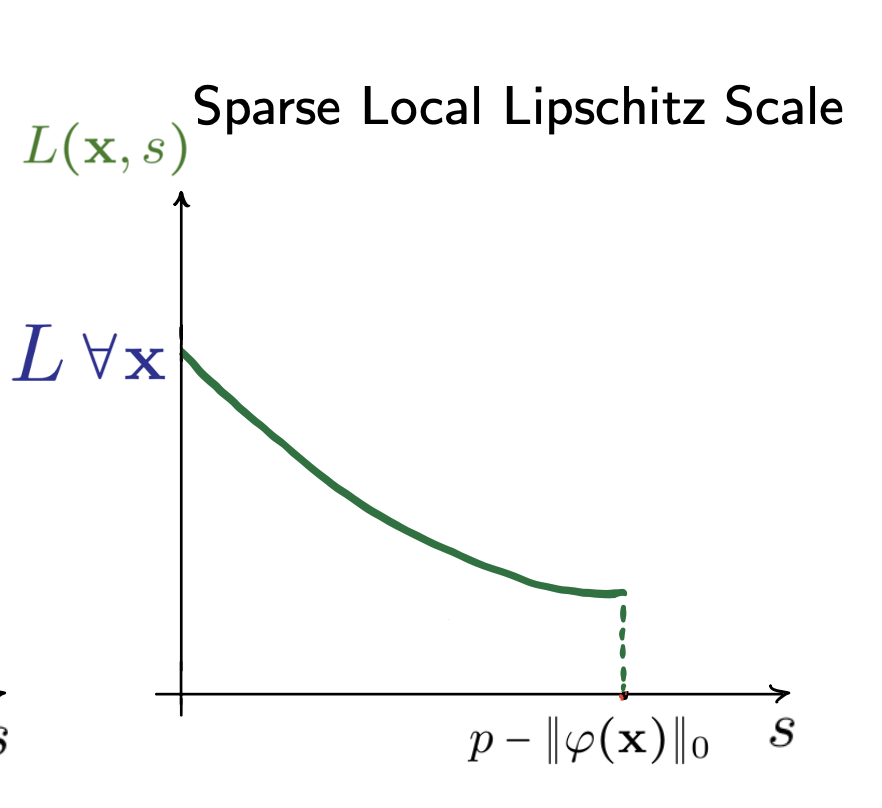
Sparse Local Lipschitzness
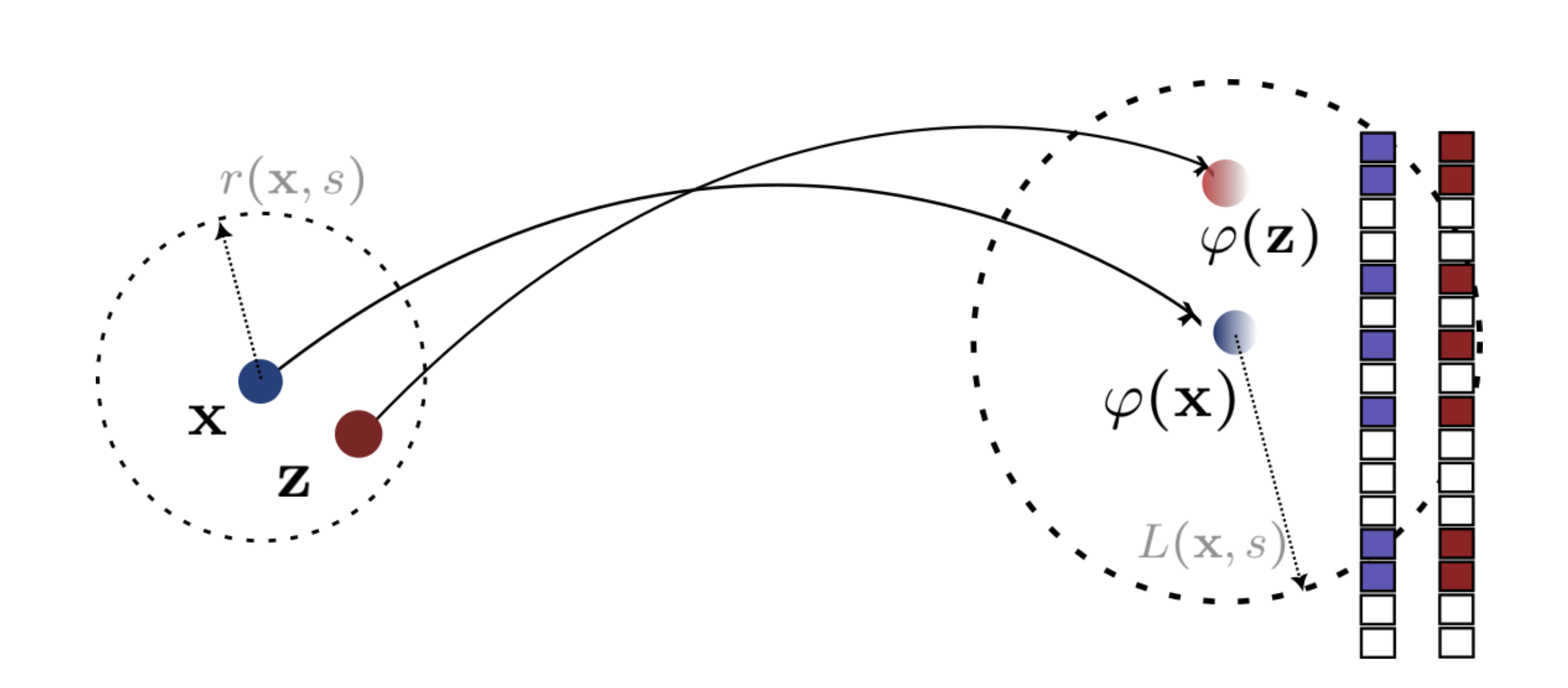
Sparse Local Lipschitzness
Example 0:
Sparse Local Lipschitzness
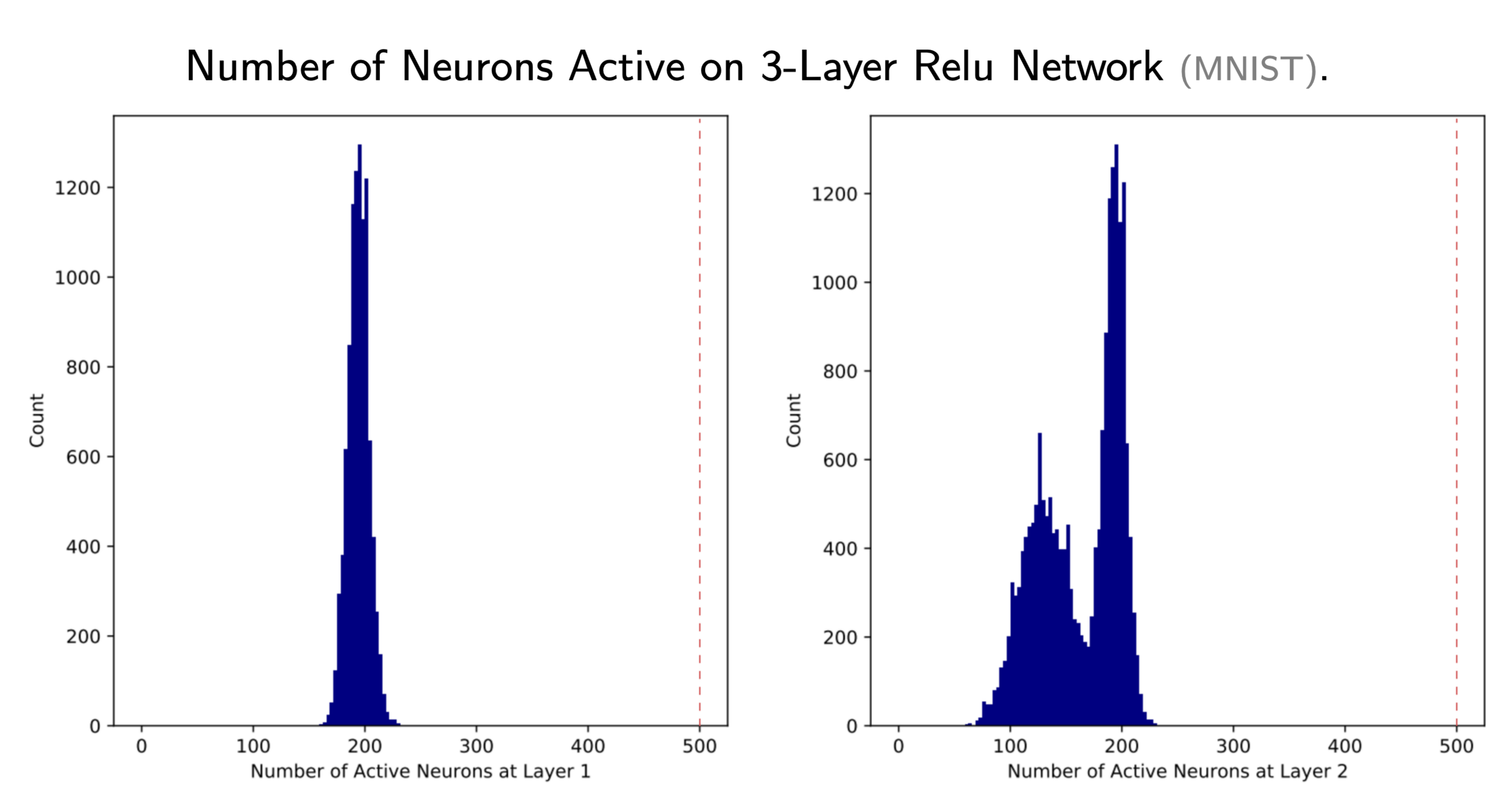
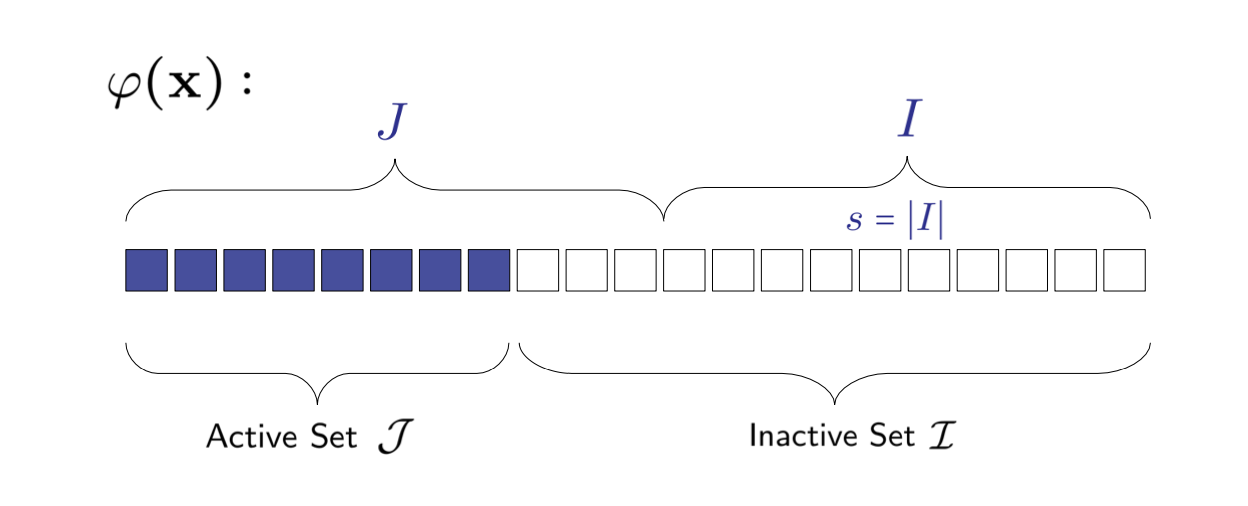
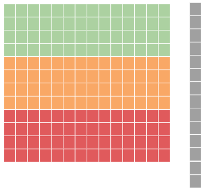
ReLU Networks are Sparse Local Lipschitz
active
weakly inactive
strongly inactive

ReLU Networks are Sparse Local Lipschitz
active
weakly inactive
strongly inactive
ReLU Networks are Sparse Local Lipschitz
active
weakly inactive
strongly inactive
active
weakly inactive
strongly inactive
ReLU Networks are Sparse Local Lipschitz
Theorem:
active
weakly inactive
strongly inactive
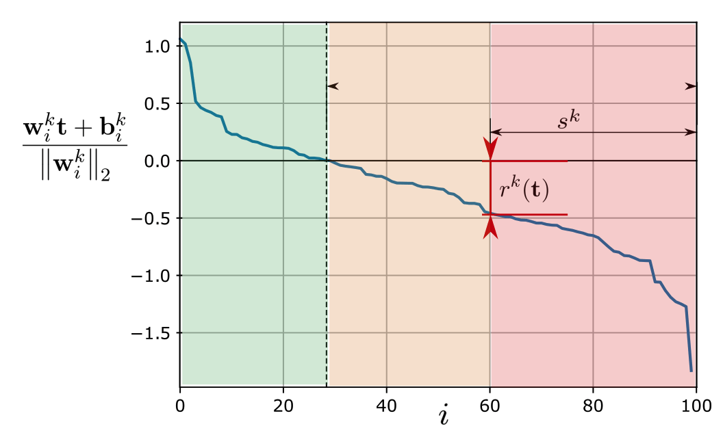
ReLU Networks are Sparse Local Lipschitz
Theorem:
active
weakly inactive
strongly inactive
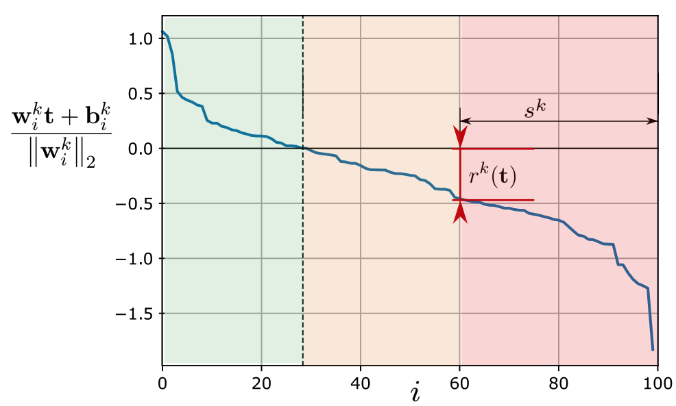
ReLU Networks are Sparse Local Lipschitz
Theorem:
Lemma:
Robustness Certificates
Theorem:
Margin vs stability
Optimal Sparsity
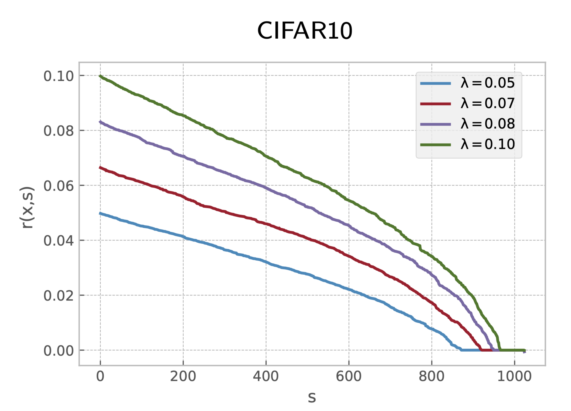
Certified Accuracy
Perturbation Energy
0.0
0.5
1.0
1.5
0.0
0.2
0.4
0.6
0.8
1.0
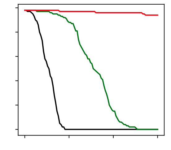


Muthukumar & S. (2023). Adversarial robustness of sparse local lipschitz predictors. SIAM Journal on Mathematics of Data Science, 5(4), 920-948.
Robustness Certificates
Generalization
Generalization Gap:
Generalization
Remark 1
Sparse Induced Norms
Generalization
more sparsity, lower sparse norms
Remark 2
Sparse Induced Norms
Generalization
Sparse Induced Norms
Lemma:
Generalization
Sparse Induced Norms
Sparse Norms Balls
Lemma:
Generalization
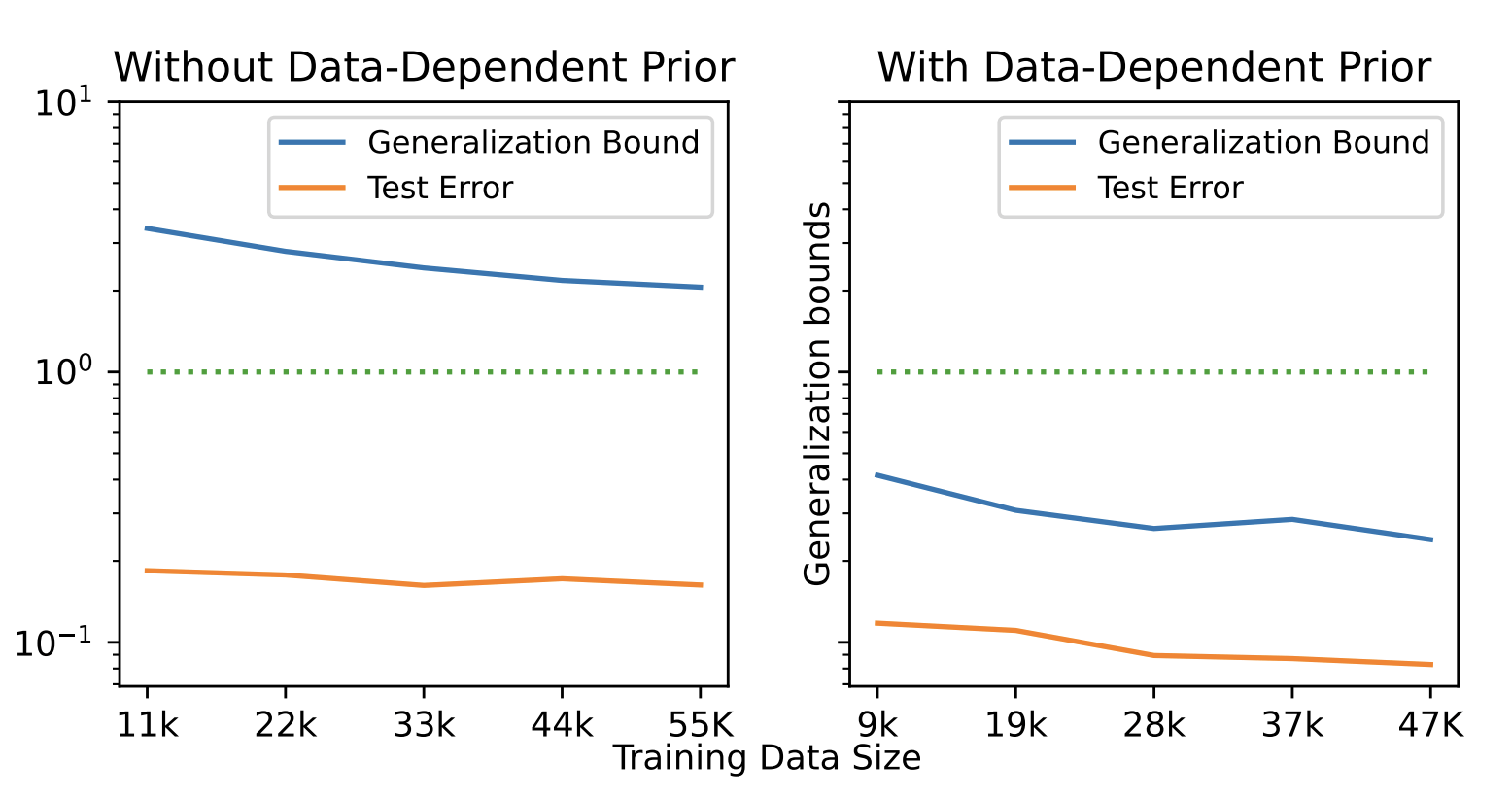
Main result (informal)
empirical (margin) risk
sparse loss
deviation from prior
sparse norms:
sparsity:
Generalization
PAC-Bayes Bounds
Observation:
Generalization
Main result (informal)
Is the empirical margin risk smaller than ?
Sparse local radius large enough (all layers) over the sample?
empirical (margin) risk
sparse loss
deviation from prior
Generalization
Main result (informal)
empirical (margin) risk
sparse loss
deviation from prior
sparse norms:
sparsity:
Generalization
Related results


Generalization
Examples
Muthukumar & S. (2023). Sparsity-aware generalization theory for deep neural networks. In The Thirty Sixth Annual Conference on Learning Theory PMLR.
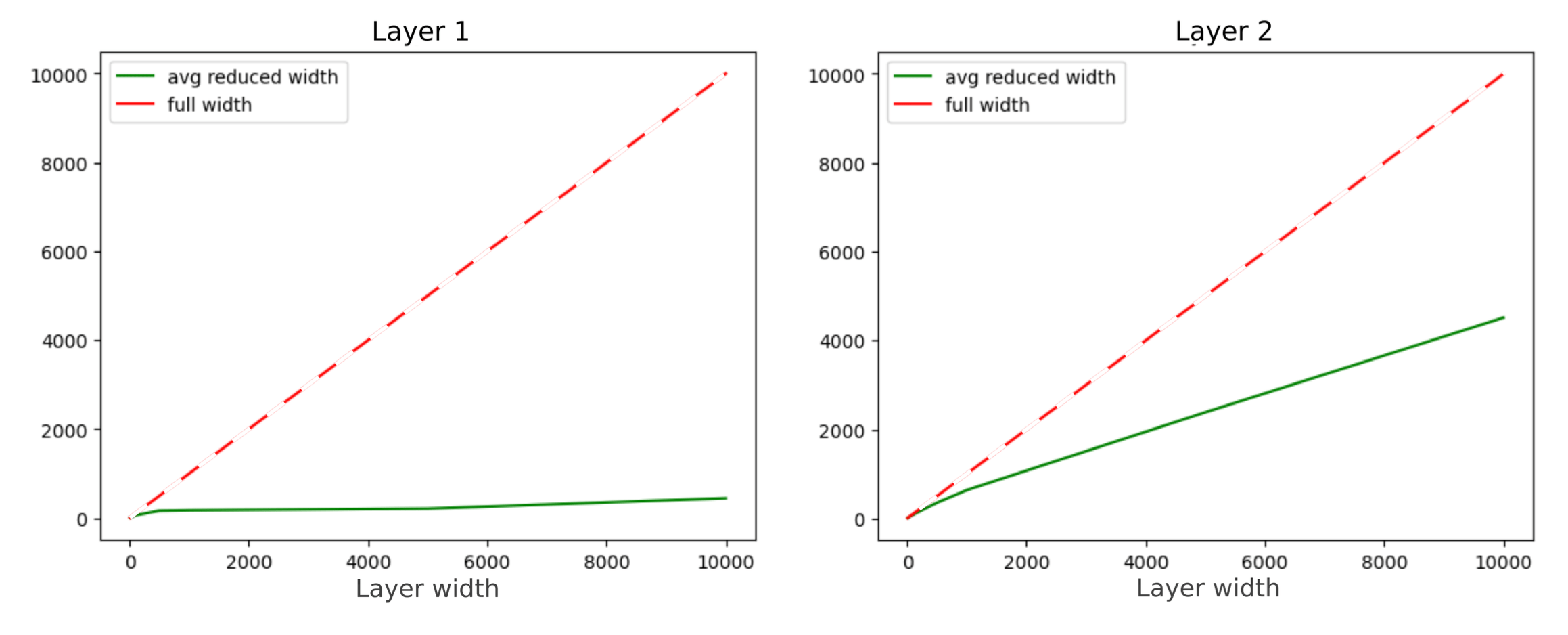
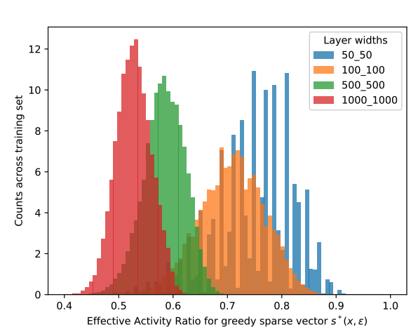
Increasing width
1. Adversarial Attacks
2. Generalization
Agenda
3. Deep models in Inverse Problems
PART I
Local Sparse LipschitznessPART II
Learned Proximal NetworksPART II
Learned Proximal NetworksLearning for Inverse Problems
measurements
reconstruction
Learning for Inverse Problems
Proximal Gradient Descent
ADMM
Learning for Inverse Problems

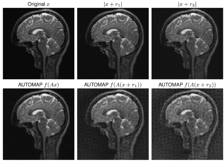
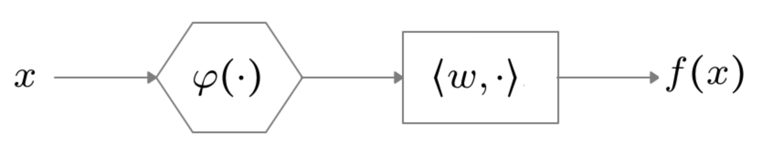
I'm going to use any neural network
... that computes a proximal, right?
That computes a proximal, right?

This is a MAP denoiser...
Let's plug-in any off-the-shelf denoiser!
Ongie, Gregory, et al. "Deep learning techniques for inverse problems in imaging." IEEE Journal on Selected Areas in Information Theory 1.1 (2020): 39-56.
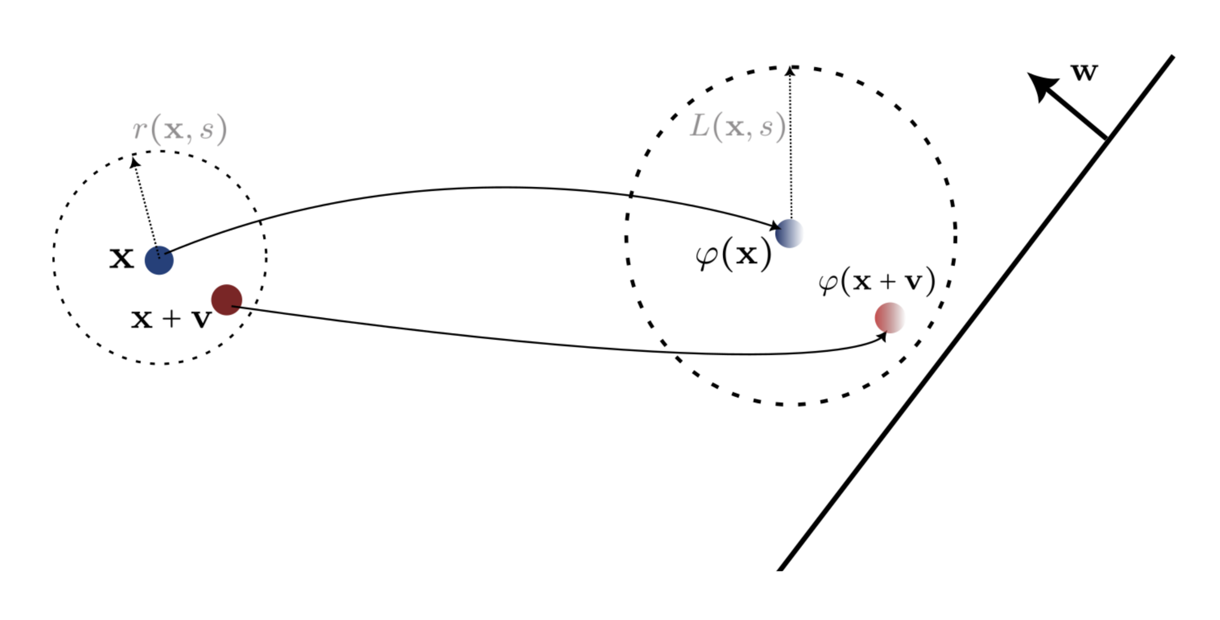
Learned Proximal Networks
Proposition
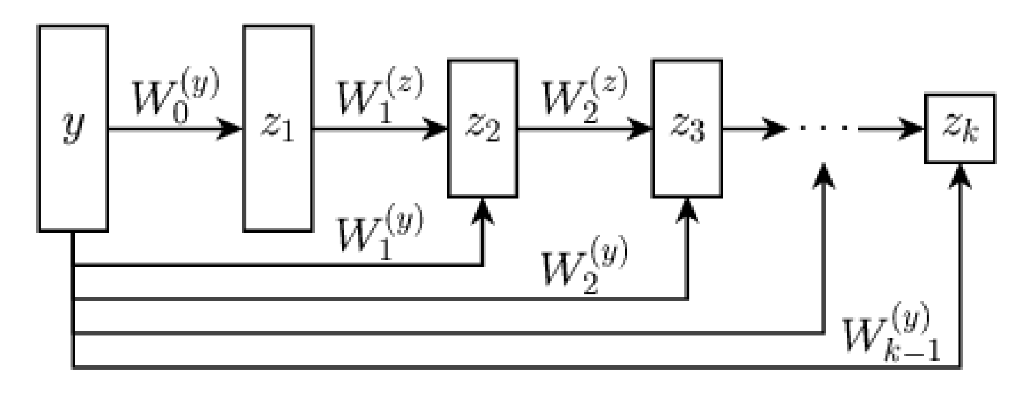
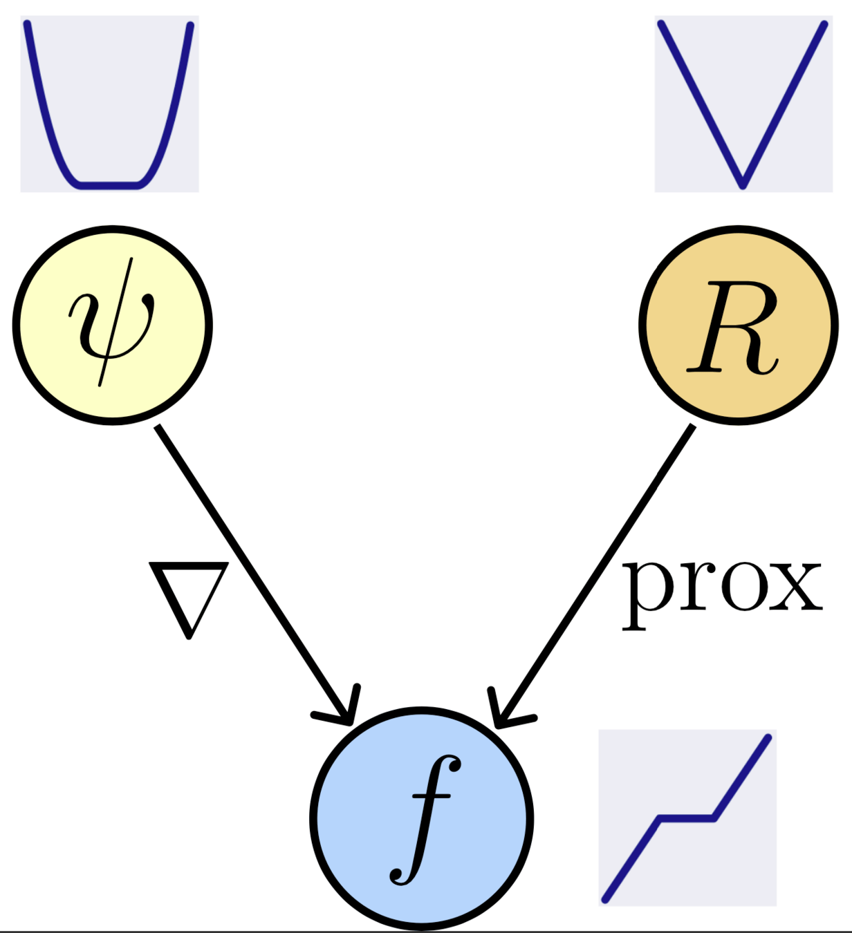
Learned Proximal Networks
Convergence:
Proximal Gradient Descent
(we don't know !)
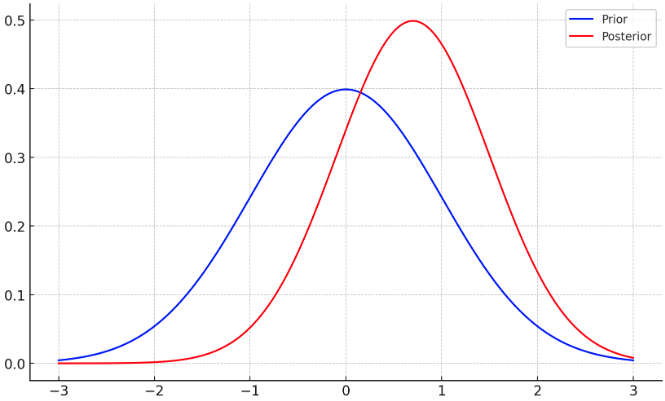
Proximal Matching
How do we train so that ?
Proximal Matching
(we don't know !)
Theorem (informal)
How do we train so that ?
Results
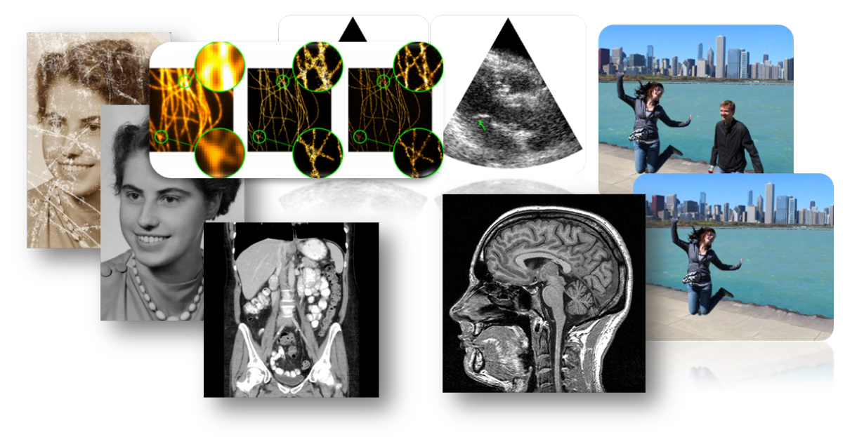
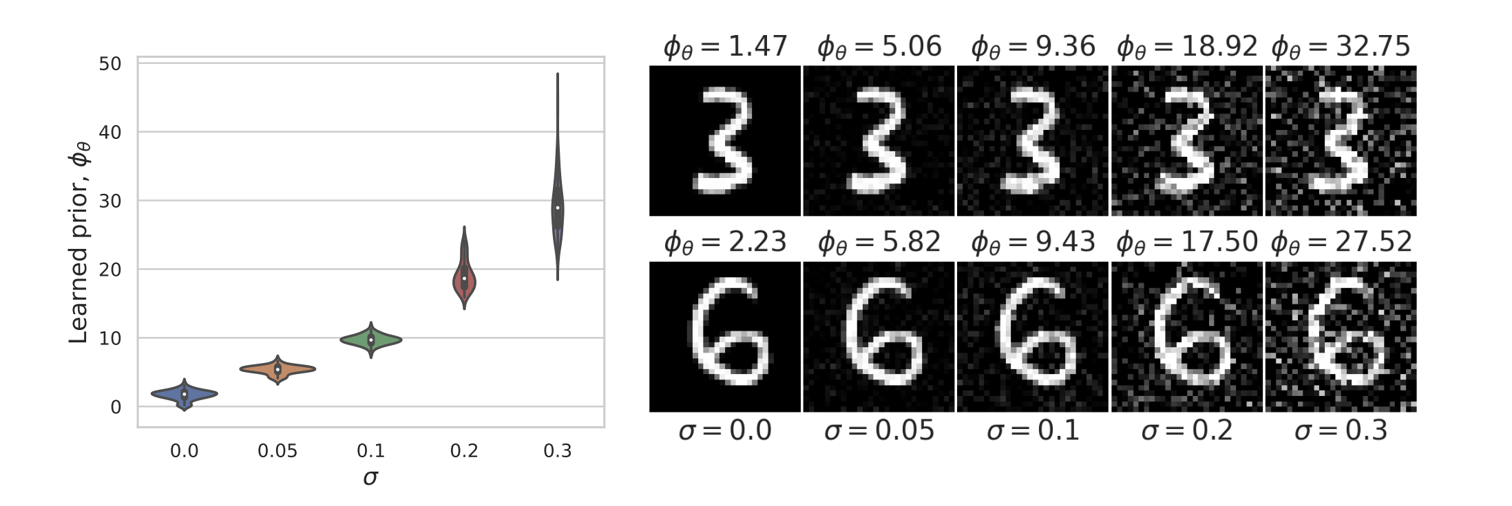
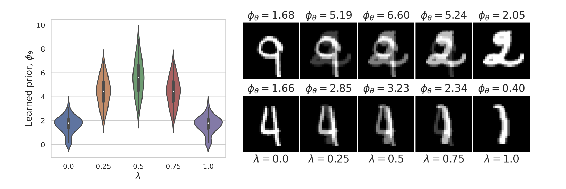
What's in your prior?
Results
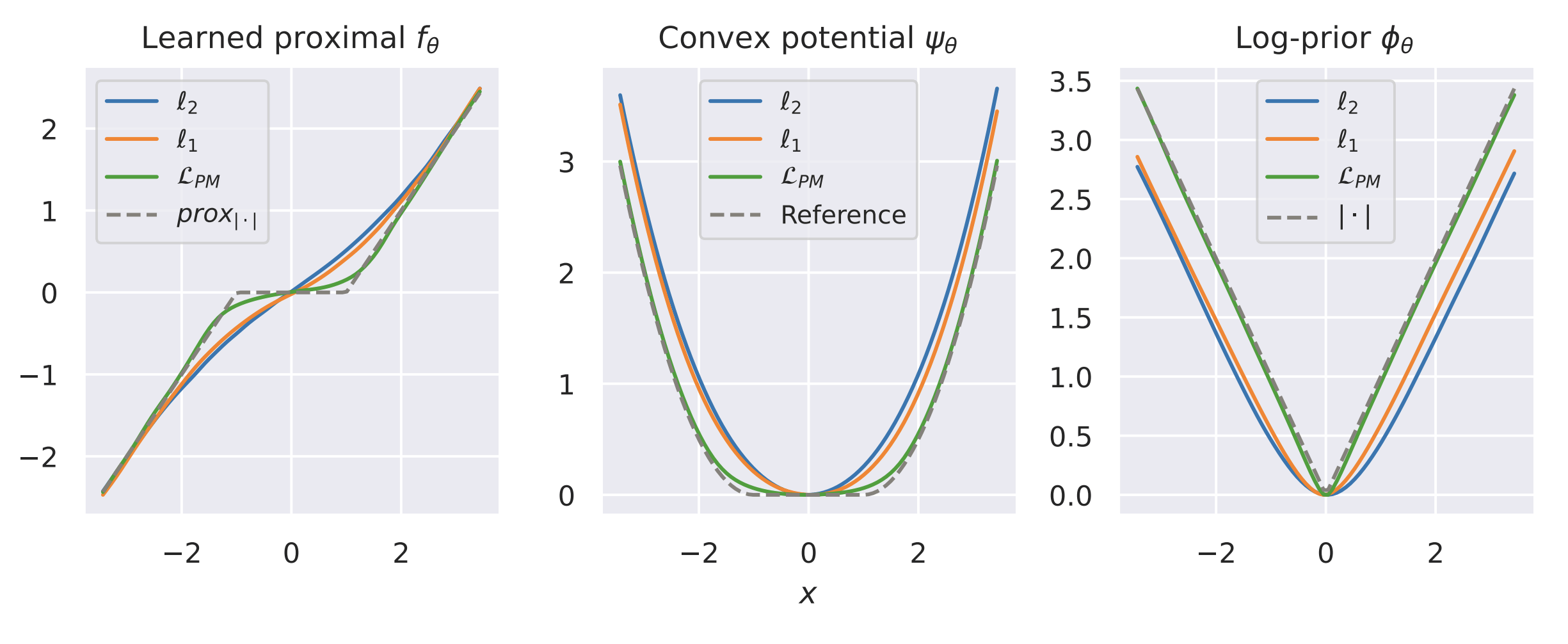
Results
MNIST
Results
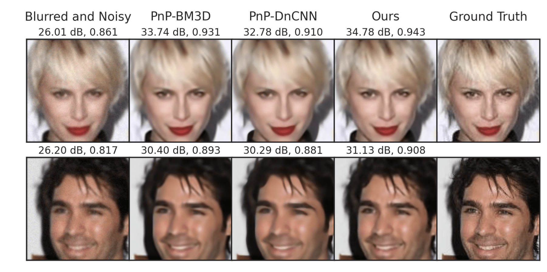
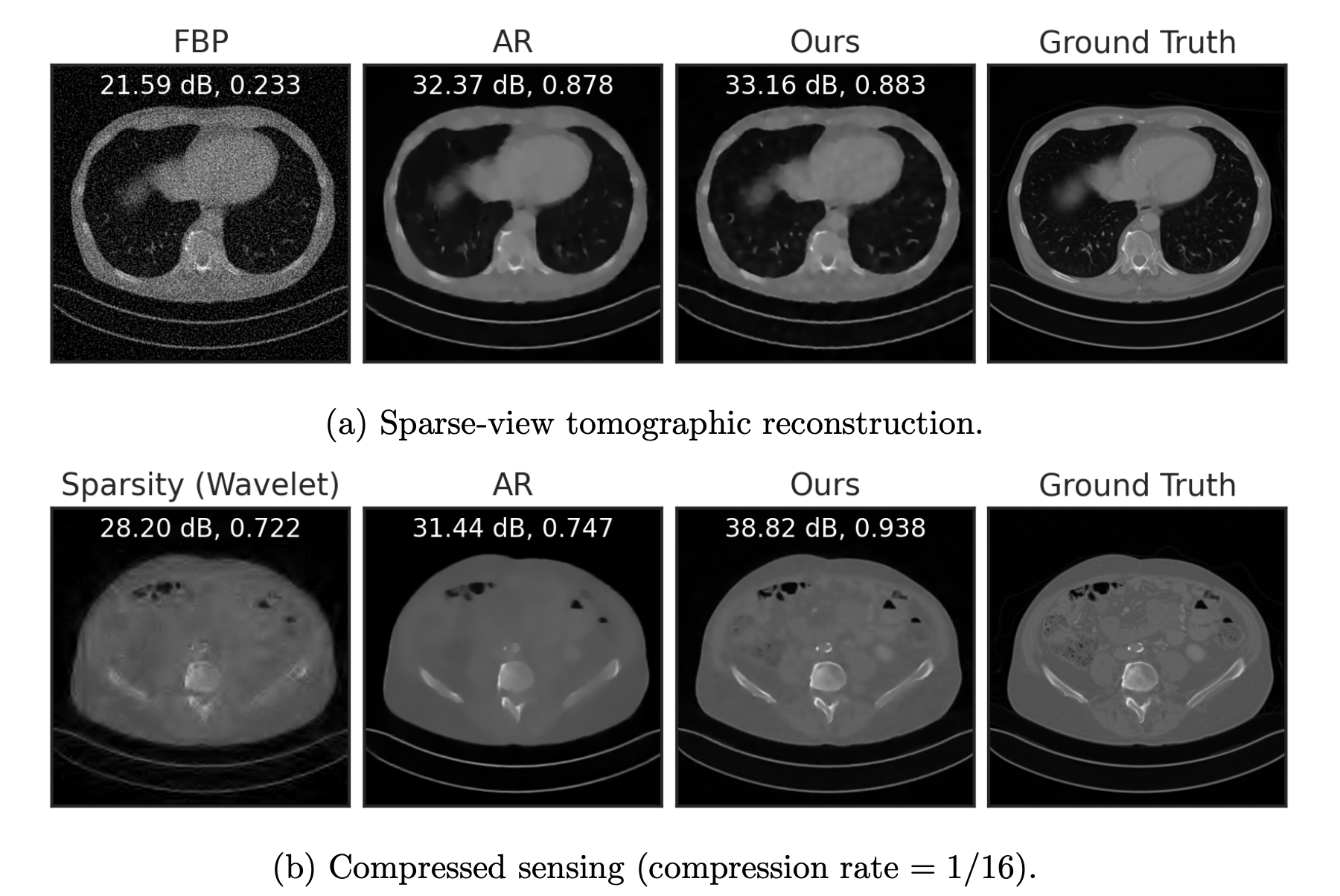
Fang, Buchanan & S. (2023). What's in a Prior? Learned Proximal Networks for Inverse Problems. arXiv preprint arXiv:2310.14344.
That is all

Ram Muthukumar
JHU
Zhenghan Fang
JHU
Sam Buchanan
TTIC
NSF CCF 2007649

NIH P41EB031771


Appendix
Example 1:
Sparse Local Lipschitzness
[ Mairal et al., '12 ]
Theorem:
[ Mehta & Gray, '13; S., Muthukumar, Arora, '20 ]