Sensing and learning in phase space
with squeezed light
Jonas S. Neergaard-Nielsen
QPIT/bigQ - Department of Physics, Technical University of Denmark


STORMYTUNE conference, Gaeta, 2024-06-19




Q. Computing
Q. Comm. + (semi)di protocols
Q. light sources
Q. sensing
Distributed sensing
Single phase estimation with squeezed vacuum
LEARNING A RANDOM DISPLACEMENT CHANNEL

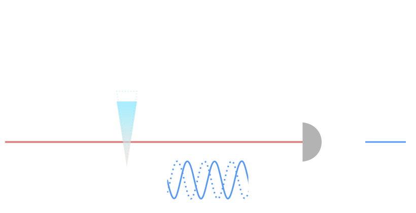
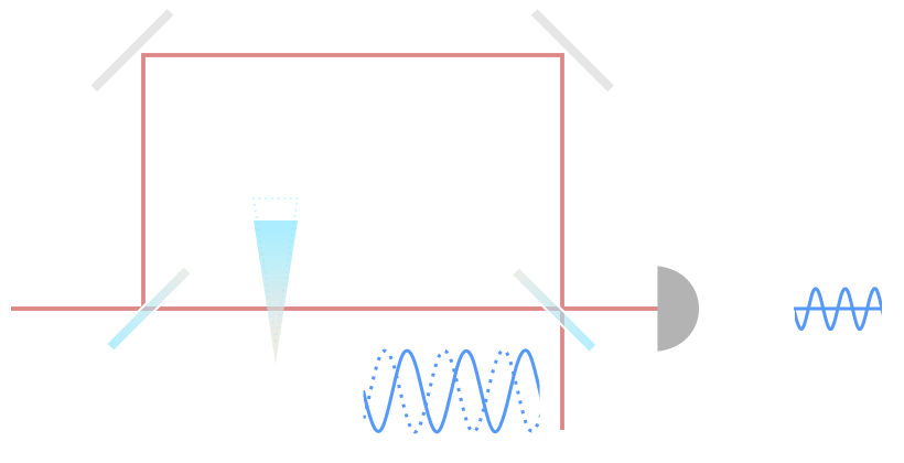
interferometric
measurement
Sensing a phase shift
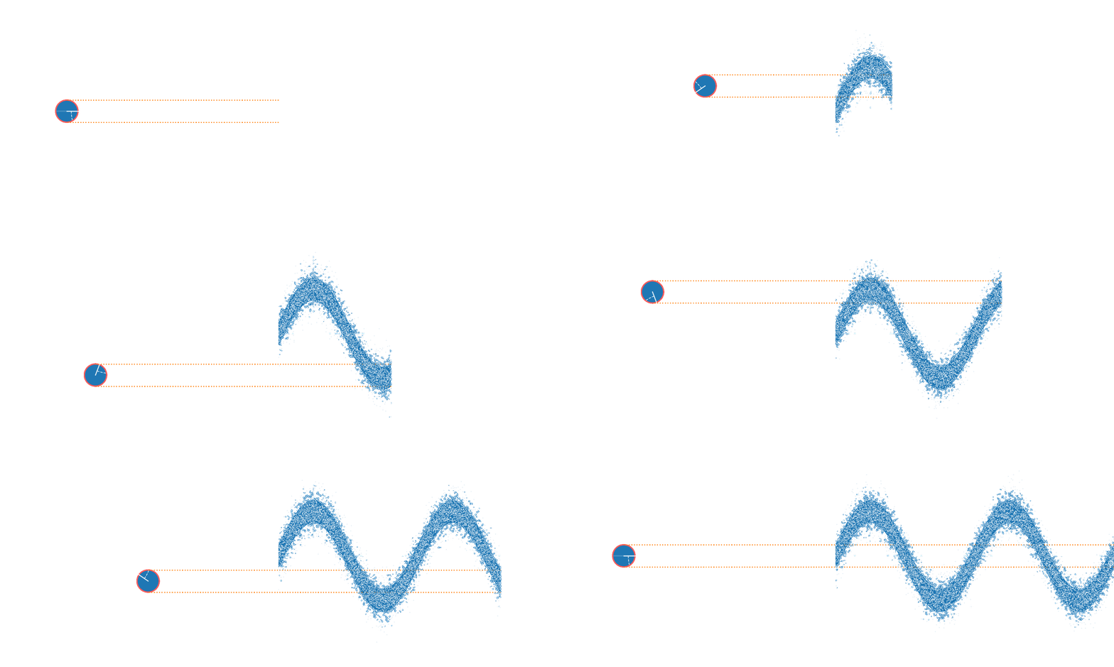
limited by quantum noise
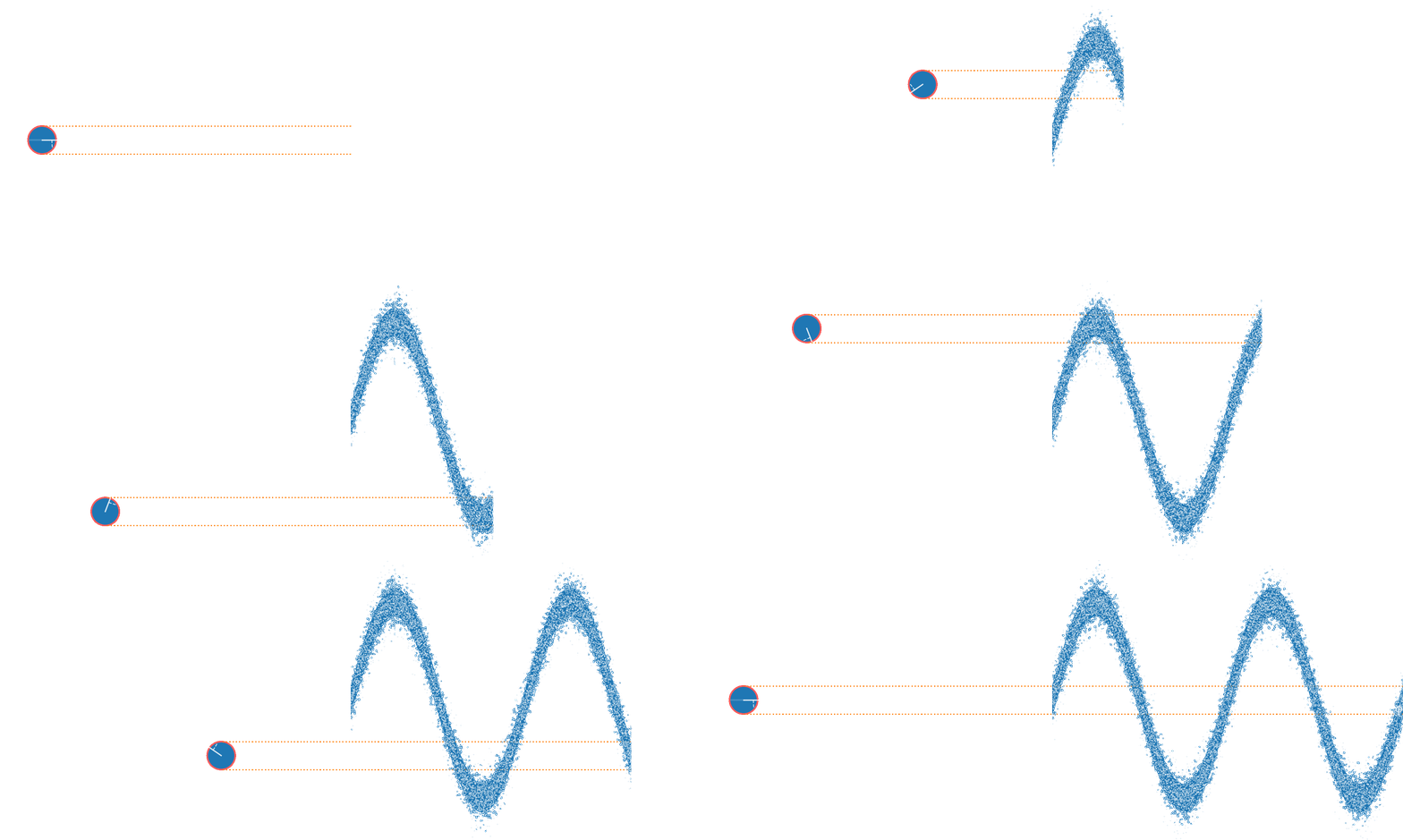
increase probe power - if possible
or squeeze...
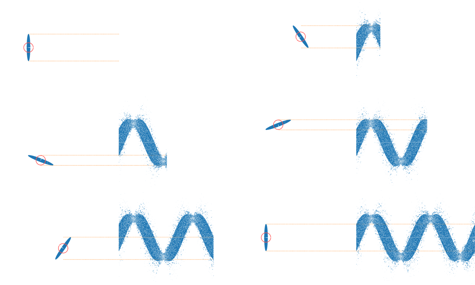
Amplitude squeezing
Phase squeezing
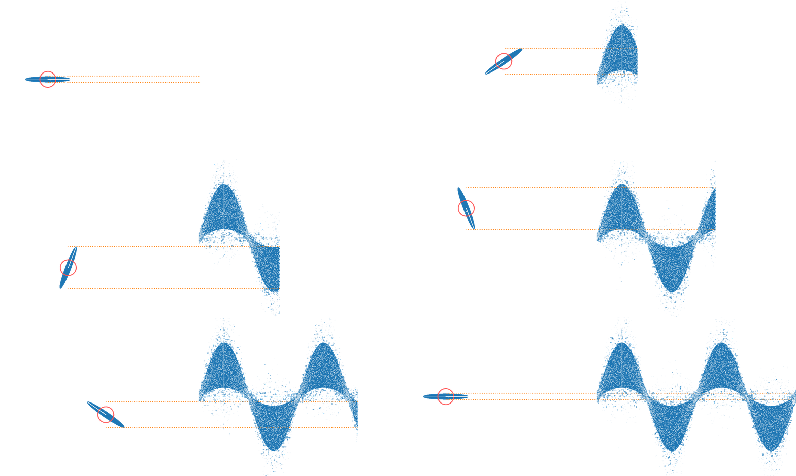
or squeeze...
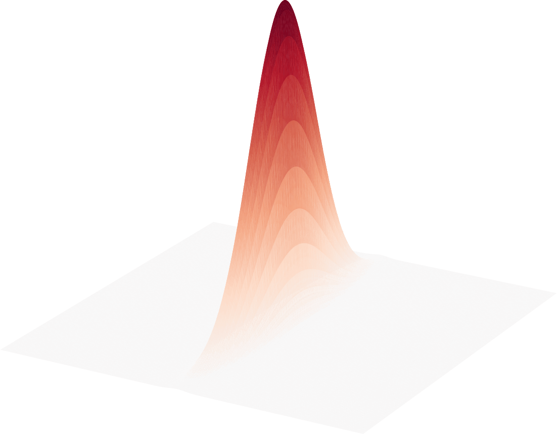
Squeezed vacuum
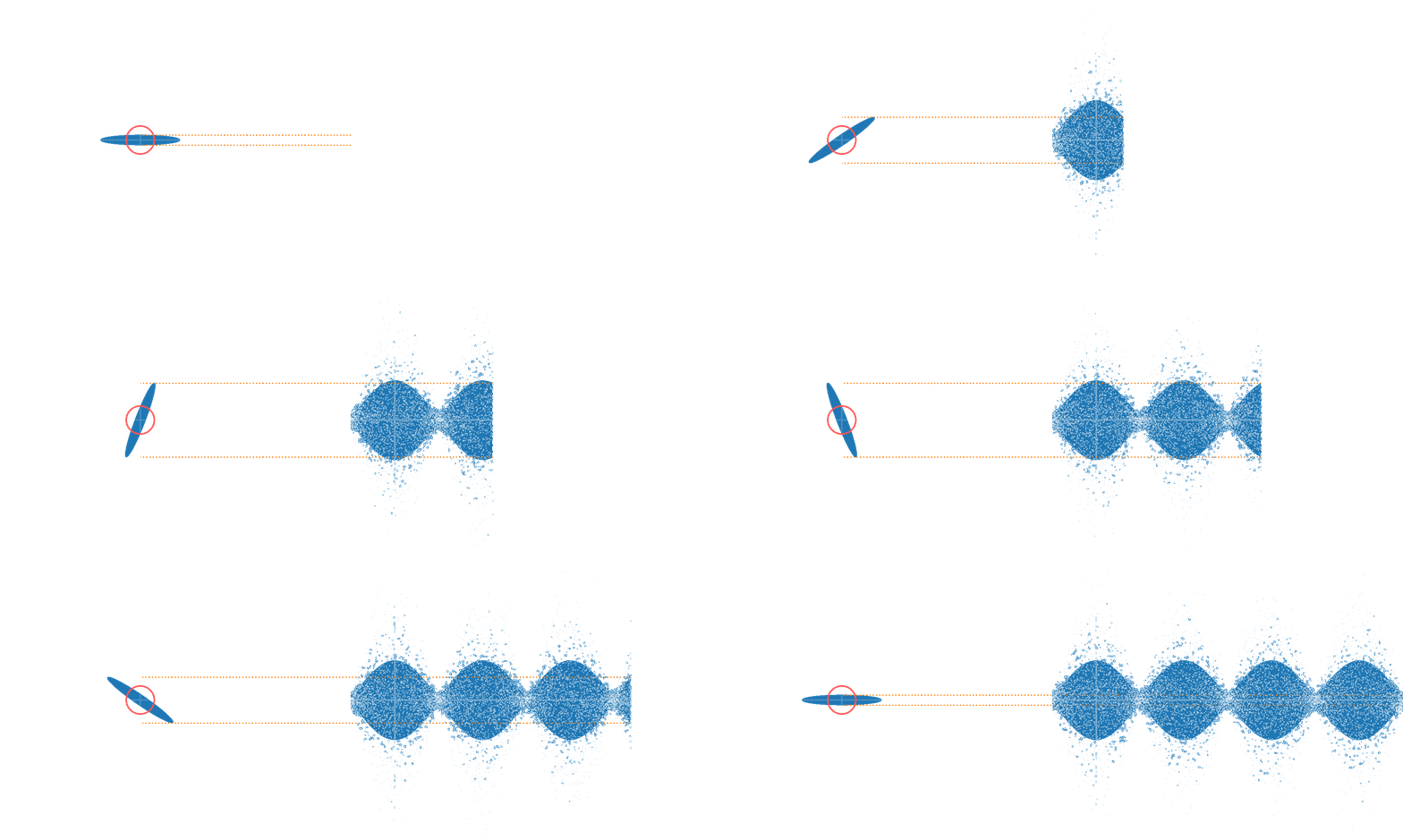
or squeeze...

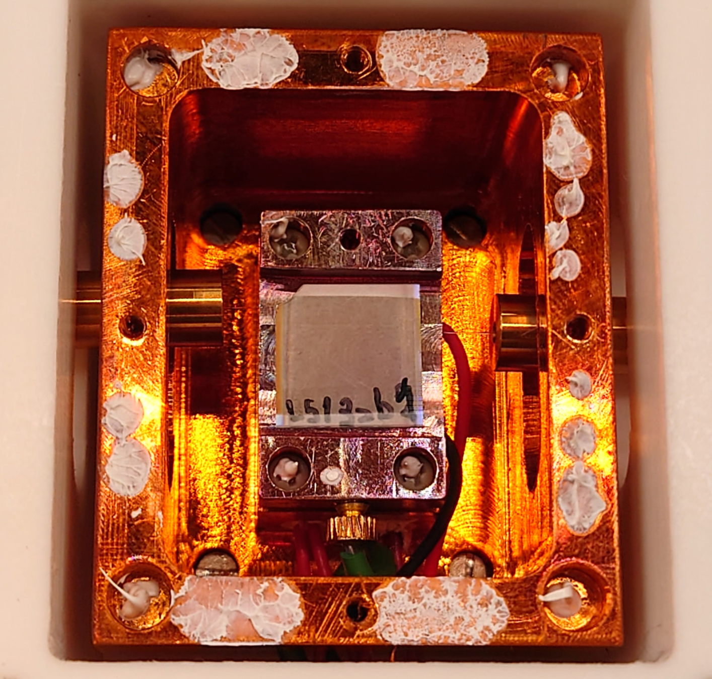
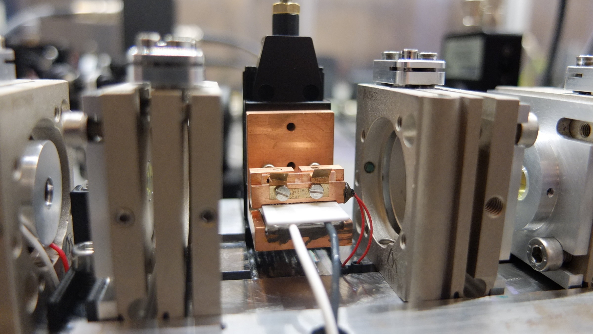
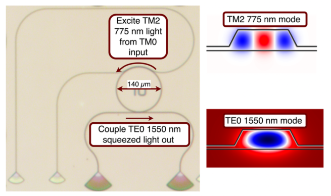
PPKTP linear
PPKTP bow-tie
PPLN waveguide

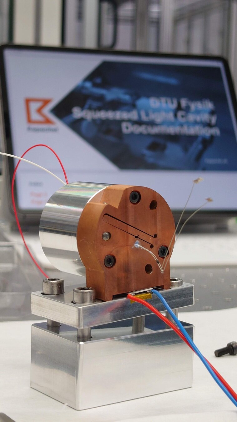


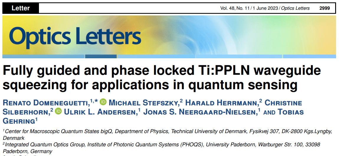
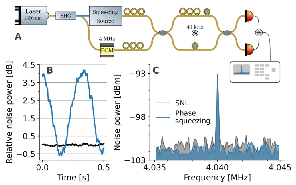

Renato
Domeneguetti
Michael
Stefszky
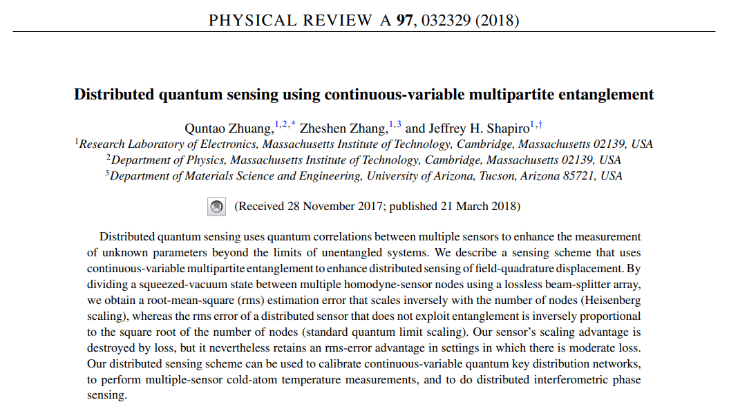
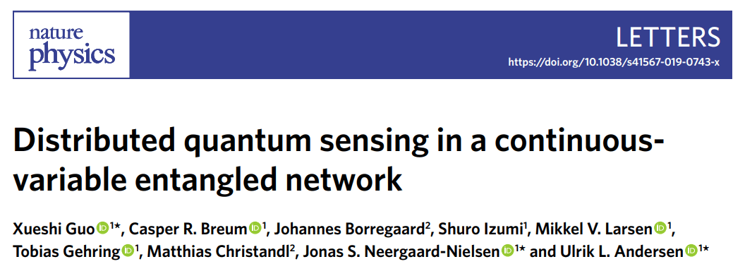
Distributed sensing


Estimate a global (distributed) parameter:
Different task

"Cheap" entanglement enhances estimation of a
global parameter of spatially separated systems
Estimate a global (distributed) parameter:
Different task




Xueshi Guo
Casper Breum
Johannes Borregaard
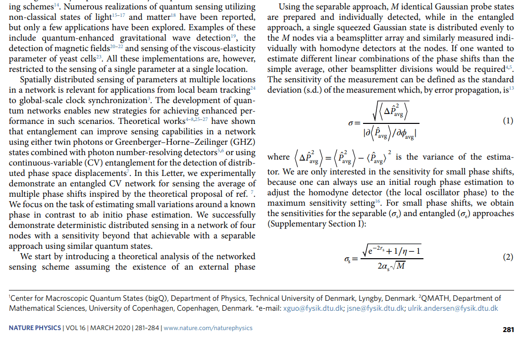
Estimate the average of multiple optical phase shifts
Homodyne detector has been pre-aligned close to the optimal phase by some rough (or adaptive) initial estimation.
For small \(\phi_i\), estimate with homodyne detection of phase quadrature:


SETTING


sensitivity \(\sigma \equiv 1/SNR\)
- minimum resolvable phase shift
HEISENBERG SCALING IN PROBE ENERGY AND # OF SITES/SAMPLES
With losses,
Heisenberg scaling disappears but sensitivity gain remains

Realistic (lossy) situation
For optimal balance between squeezed and coherent photons:


Experiment
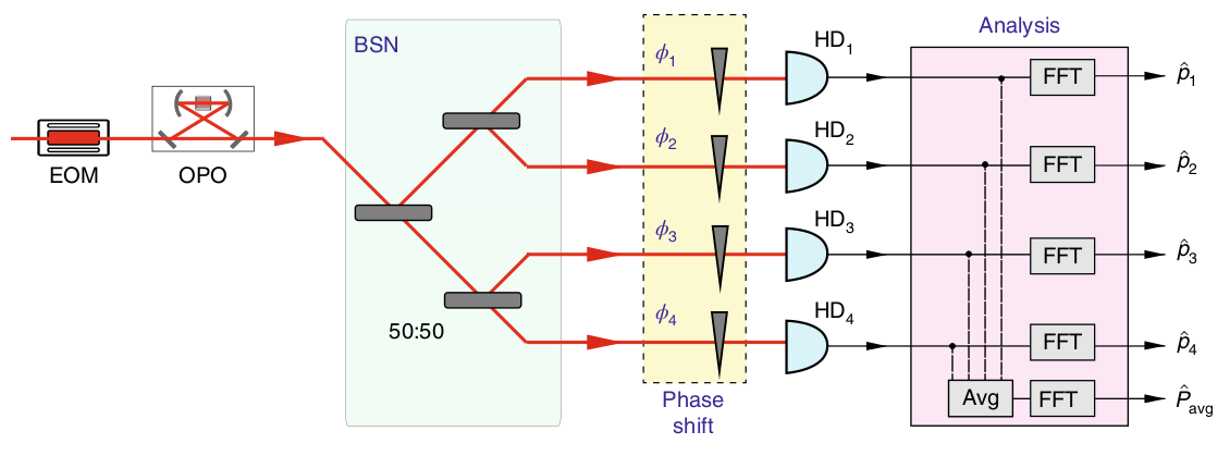


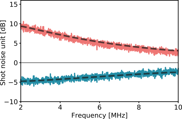
Measured sensitivities

Measured sensitivities
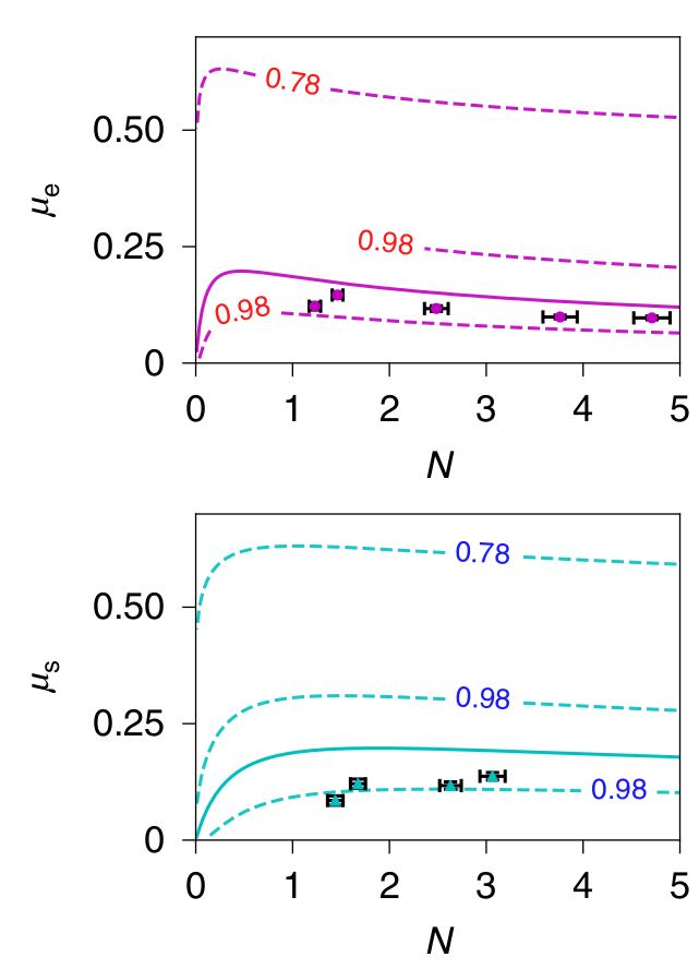
Optimised photon number balance
single phase estimation with squeezed vacuum


Single phase sensing - improving sensitivity
estimator:
sensitivity:
photons per probe:
displaced
squeezing
squeezed
vacuum
estimator:
sensitivity:
photons per probe:

Jens AH Nielsen
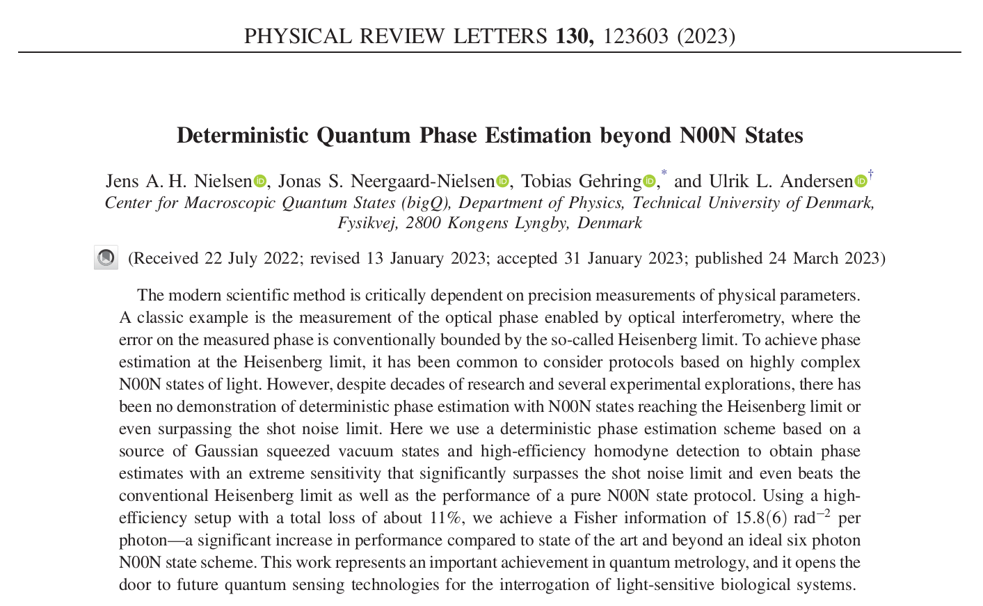
Comparison with Noon states


Comparison with Noon states
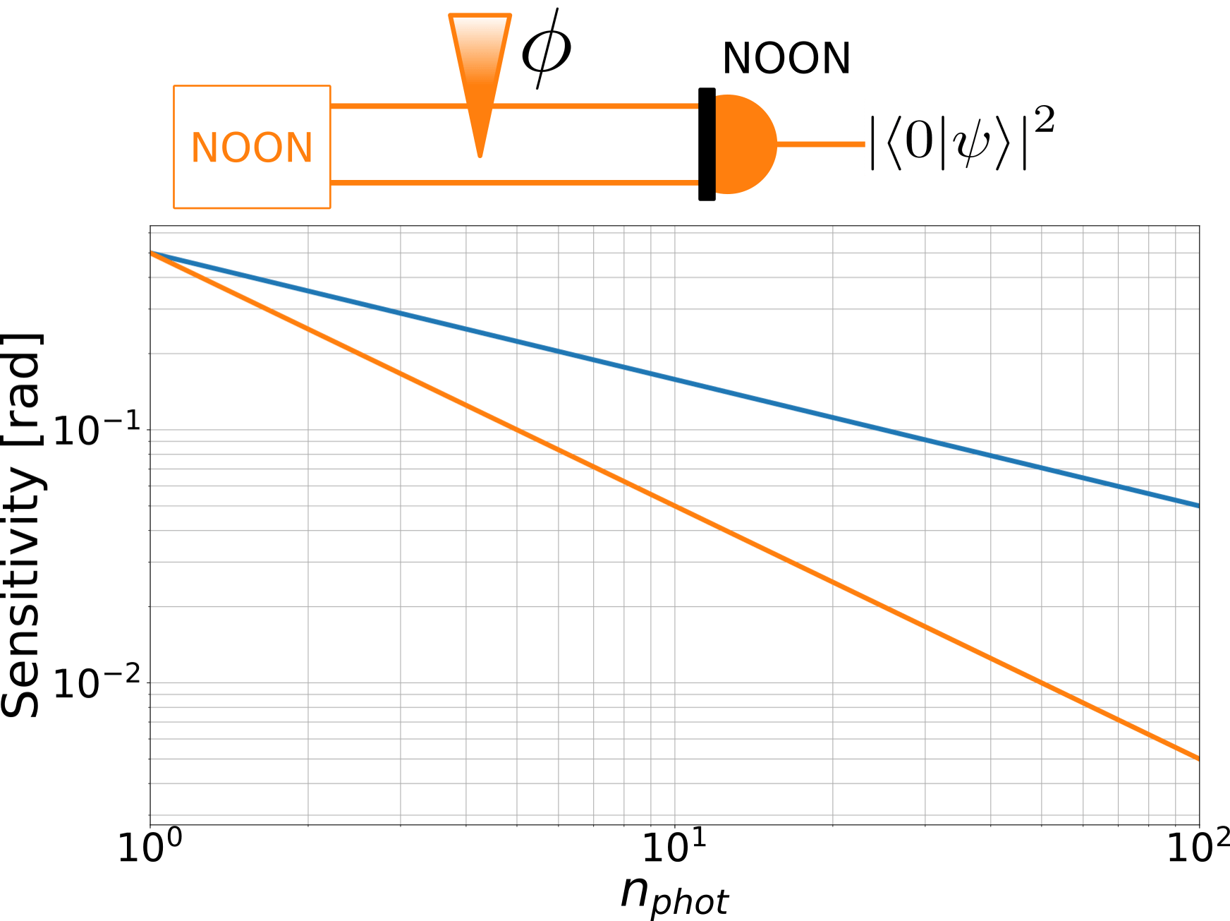
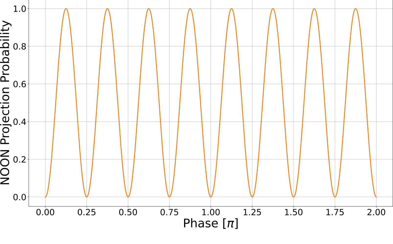
Comparison with Noon states
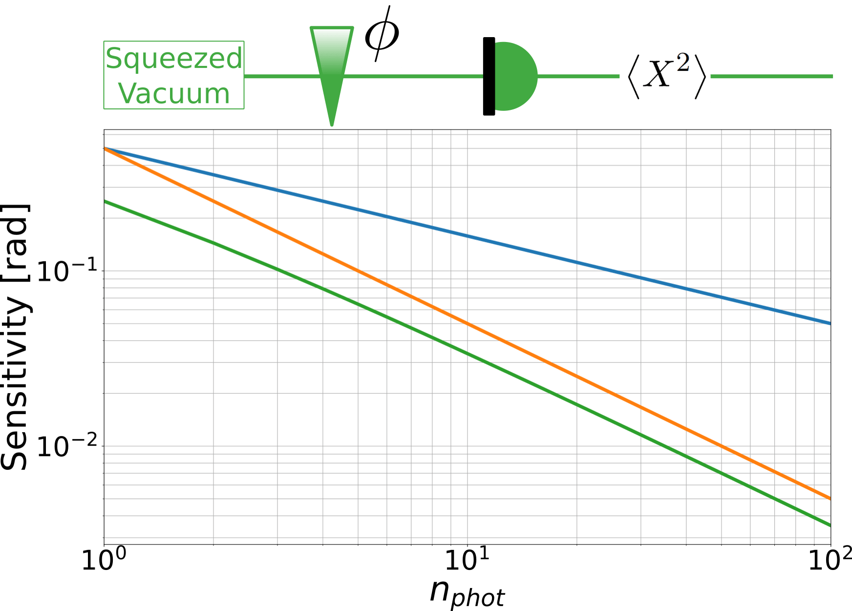
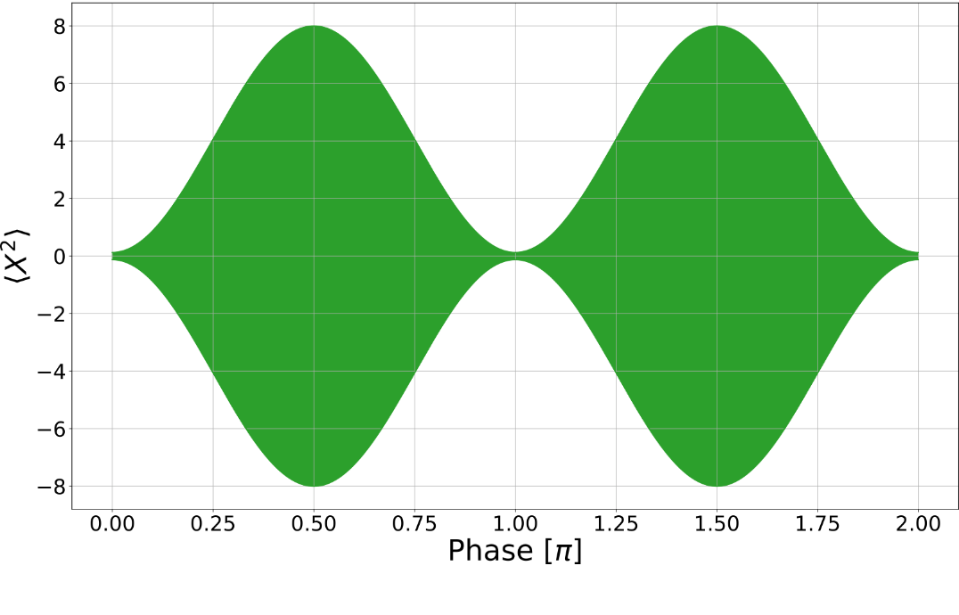
Experiment
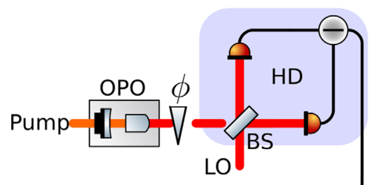
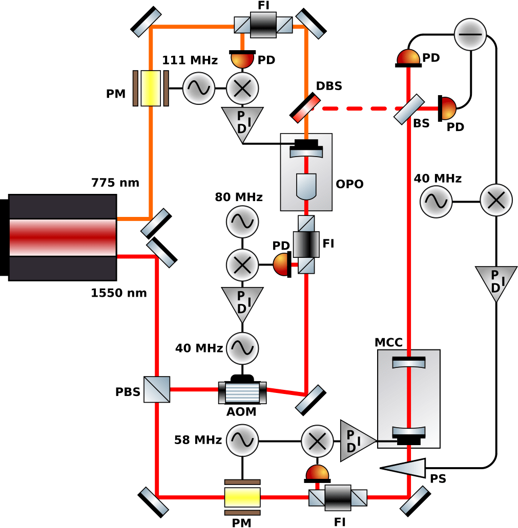


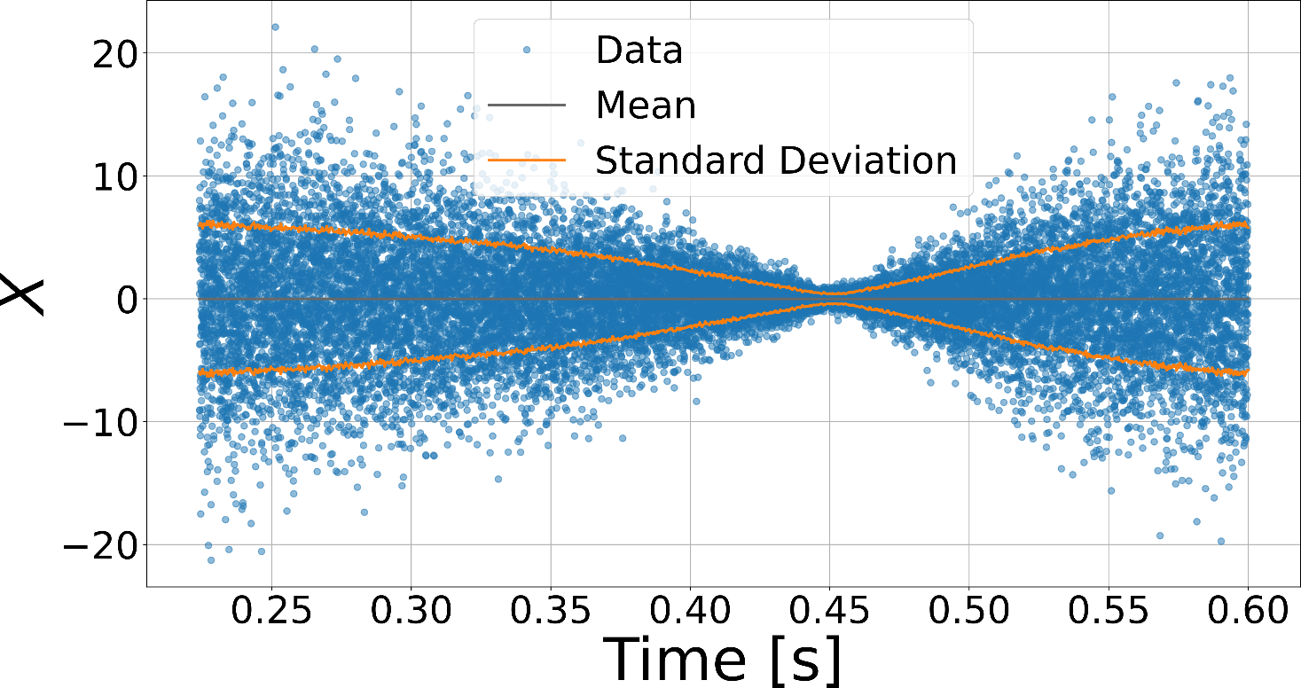

Experiment
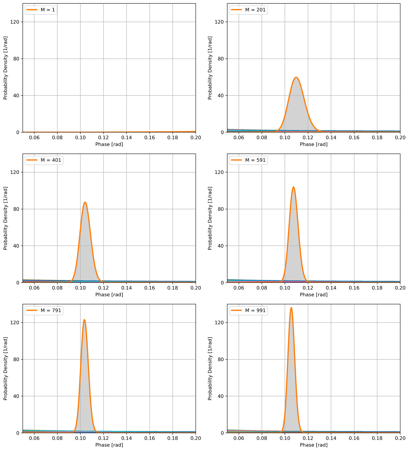
Bayesian updating of the likelihood of \(\phi\):
- Estimate is \(\hat\phi = \text{arg max }P(\phi|\{P_i\})\),
- Sensitivity is \(\sigma = \sqrt{\text{Var }P(\phi|\{P_i\})}\)
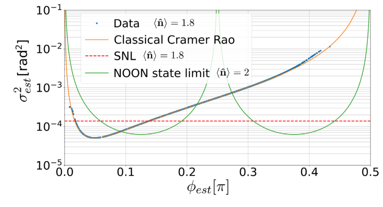
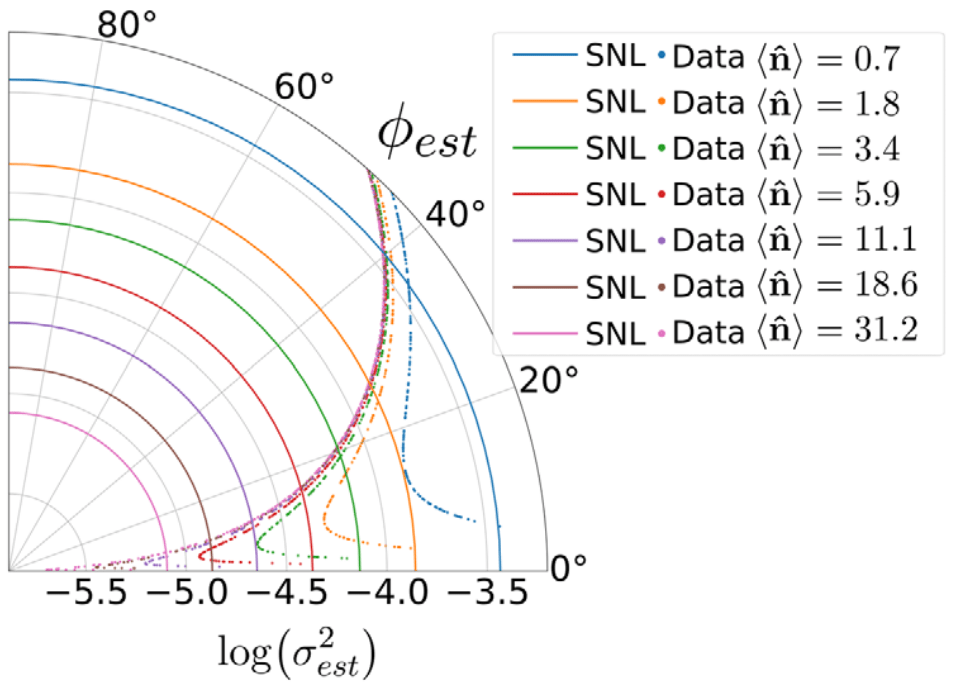
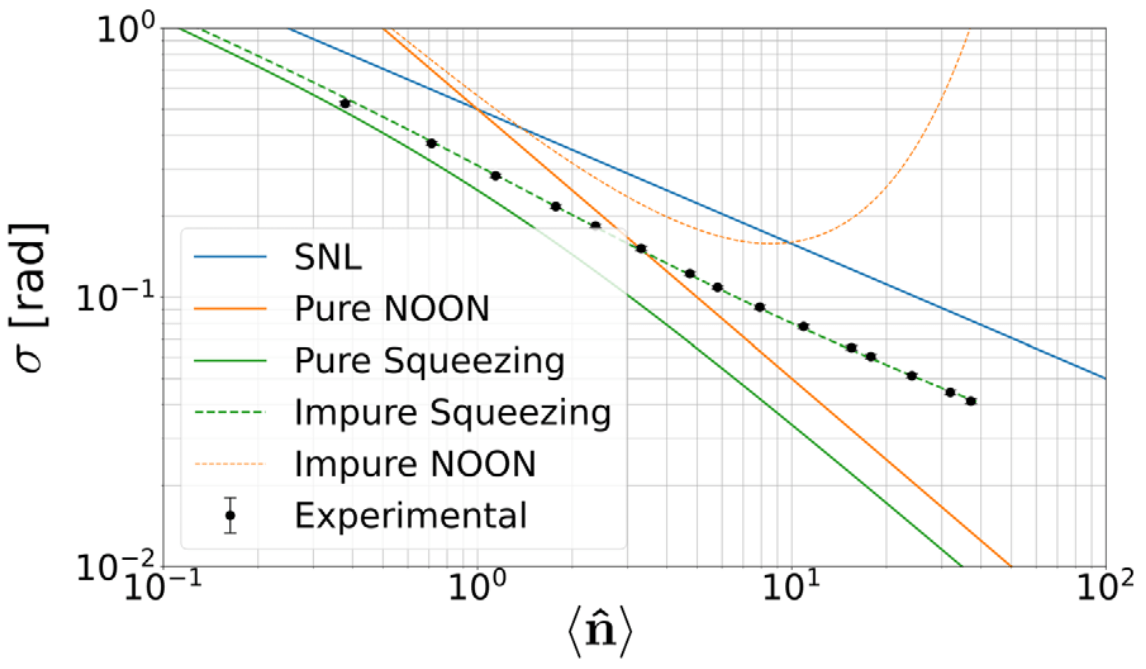
Scaling of the sensitivity

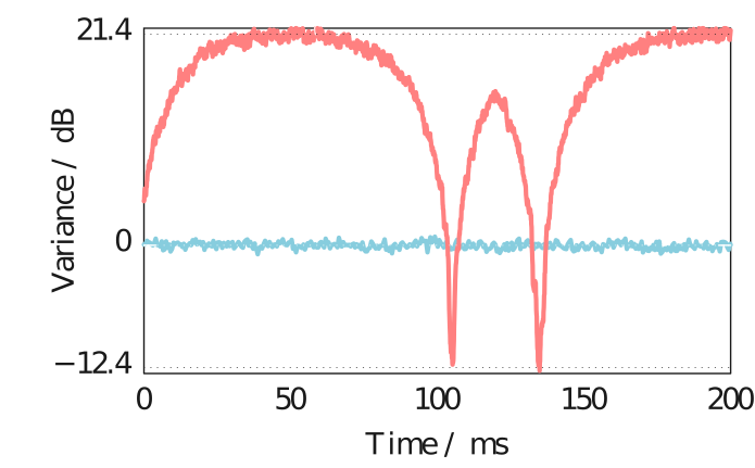
demo of the "deterministic" in the title
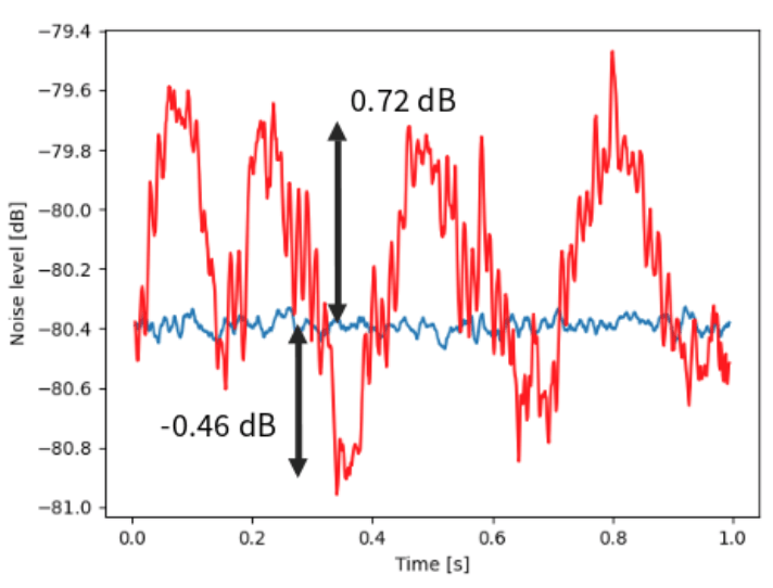
Applying a weak 3 kHz phase modulation,
we recover this signal in the recorded trace and spectrum
Learning a random displacement channel
(work in progress)
New scenario
Channel:
Dynamics:
Goal:
Small phase shift (\(\approx\) p-displacement) on \(n\) modes
Static - can be probed repeatedly
Estimate average phase shift
Distributed sensing
x- AND p-displacements on \(n\) modes
Random - varies shot to shot, distribution \(p(\alpha)\)
Learn \(p(\alpha)\)
Channel:
Dynamics:
Goal:
Channel learning
x- AND p-displacements on \(n\) modes
Random - varies shot to shot, distribution \(p(\alpha)\)
Learn \(p(\alpha)\)
Channel:
Dynamics:
Goal:
Channel learning
EPR state
← Squeezed probes are no longer very useful
Take inspiration from dense coding →
New scenario
Random displacement Channel learning

Random displacement Channel learning
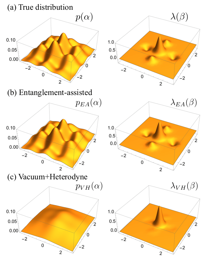
Alternative description in terms of \(p\)'s characteristic function \(\lambda\):
Large \(\beta\) values ⇒ fast ripples in \(p(\alpha)\)

Random displacement Channel learning

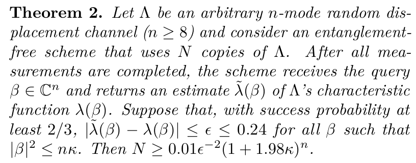
Aim:
Sample the channel \(N\) times, obtaining \(n\)-mode samples \(\{\zeta_i\}\),
after which an estimate \(\tilde\lambda(\beta)\) can be obtained with sufficiently low error for any \(\beta\) within a range \(|\beta|^2\le \kappa n\).
For the entangled scheme, an unbiased estimate is
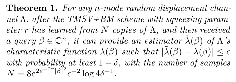
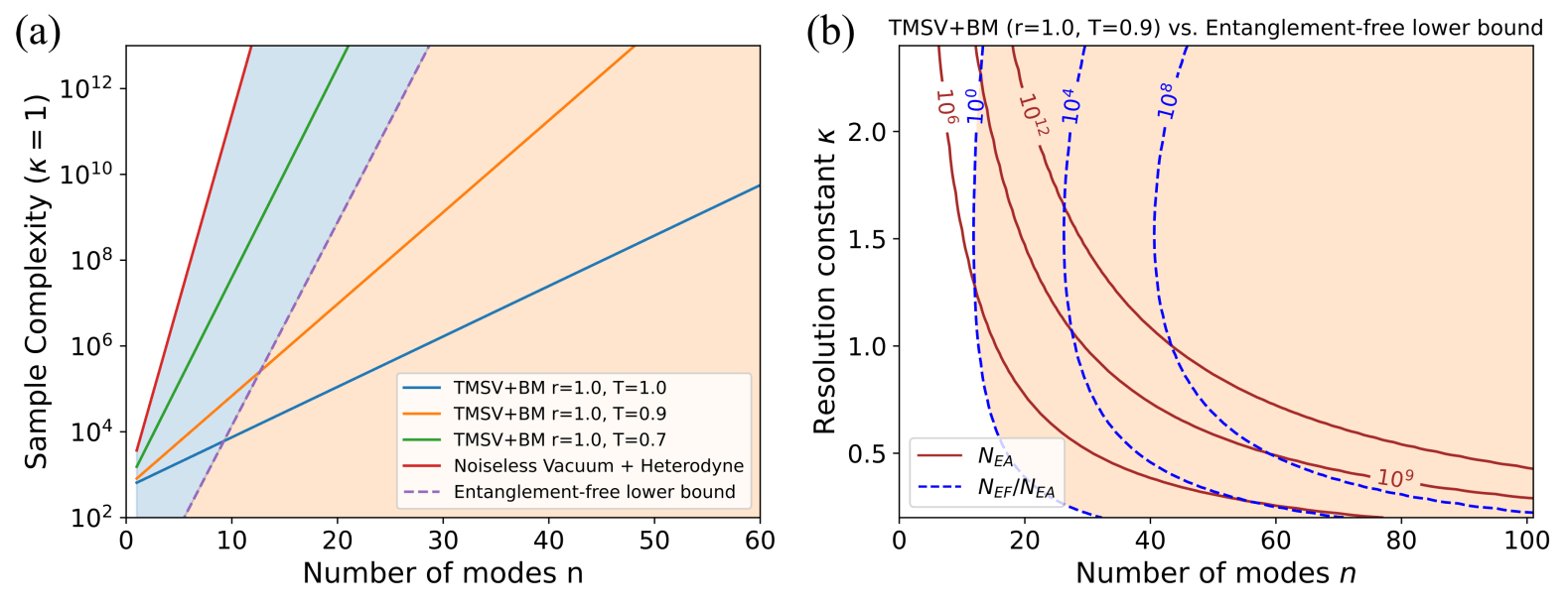
\(e^{2e^{-2r}|\beta|^2} \approx 5\cdot10^8\) for \(|\beta|^2=10\) and \(r=0\), but \(\approx 7\) for \(r=1.15\) (10 dB squeezing)
Random displacement Channel learning



Random displacement Channel learning


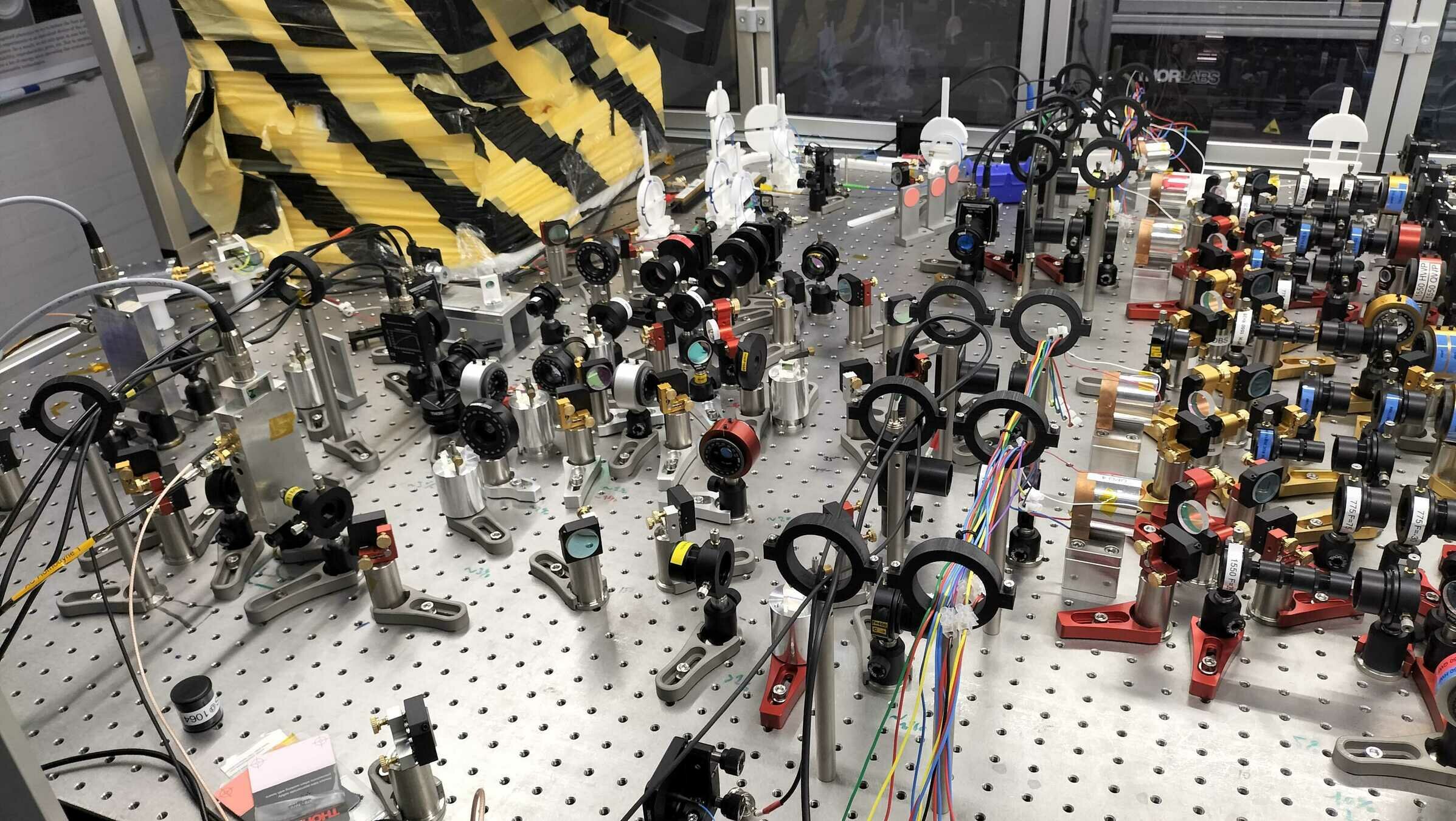
implementation
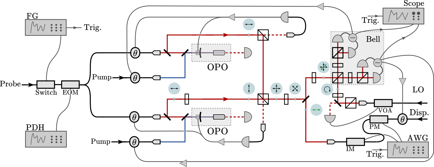
EPR state in the H/V basis,
n modes separated in time
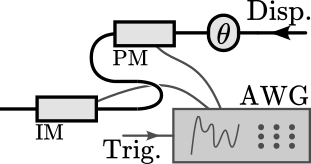
Displacement
implementation

implementation
\(n\) modes consecutive in time
Each mode: 1 µs long, 1 MHz bandwidth around 7 MHz sideband
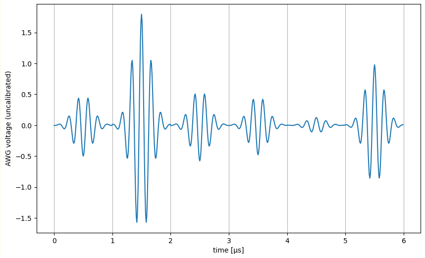
Example:
one random sample for \(n=3\)
Simulation
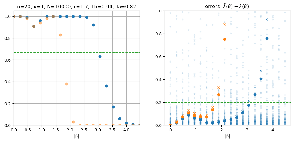
success probability of
estimating \(\lambda(\beta)\) with error <0.2
for randomly sampled \(\beta\)
\(\lambda(\beta)\) estimation errors
· mean
× 2/3 quantile
classical
entangled
Preliminary results
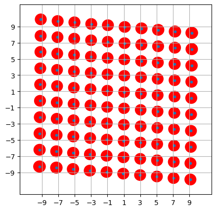
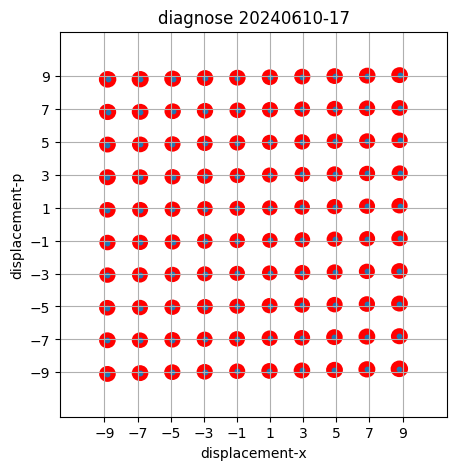
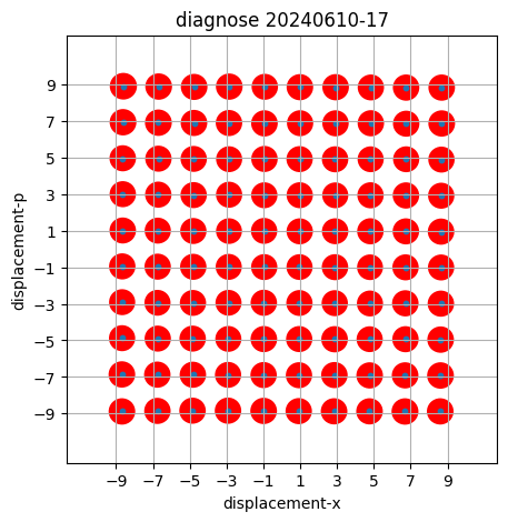
Well-calibrated displacements over wide range in phase space
without entanglement
with entanglement
sometimes cross-talk
between IM and PM
Preliminary results
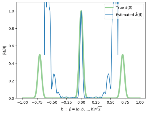
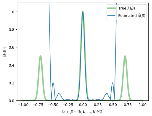
Very first attempt at learning a random \(\Lambda\) this Monday
- not successful, but we can see what to fix

"3-peak channel":
Here, \(\gamma = \frac{1}{\sqrt{2}}(1,1,\ldots,1)\)
diagonal slice through 40-dim \(\beta\)-space
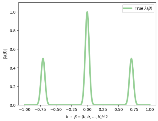
Our goal
1. Show accurate reconstruction of an \(n\) mode channel, much improved by squeezing
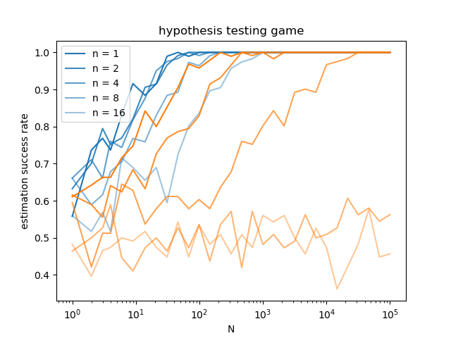
2. Show scaling advantage through a hypothesis testing game:
- Alice prepares a channel for Bob, choosing with equal probability between
a) a symmetric Gaussian
b) a 3-peak channel with a randomly chosen \(\gamma\) (location of side-peaks)
- Bob learns the channel, after which Alice provides him the value of \(\gamma\);
Bob must now guess whether the channel was a) or b)


Zhenghao Liu
Jens AH Nielsen
Emil Østergaard
Romain Brunel
Oscar Boronat
Axel Bregnsbo

Ulrik Andersen
The team
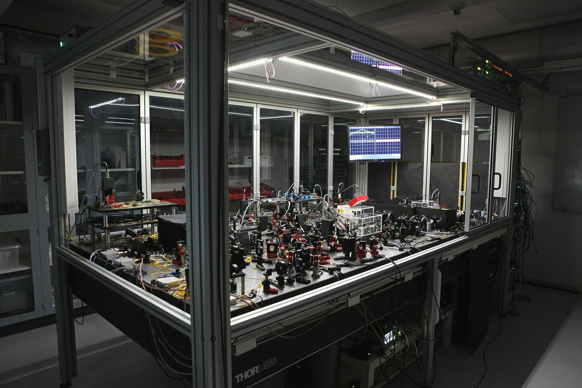


Experiment
