Harmonic equiangular tight and their combinatorial generalizations
frames
's

John Jasper
South Dakota State University
Outline
1. Projective packings:
What do we mean by "vectors that are well spread out"?
2. Harmonic equiangular tight frames:
Using groups to build sets of vectors that are optimally spread out.
3. Getting rid of the group part 1:
That's not a group, that's a block design.
4. Getting rid of the group part 2:
Who needs a group? Association schemes can do the job.
Part 1.
Projective packings
What collections of vectors/lines are as spread out as possible?
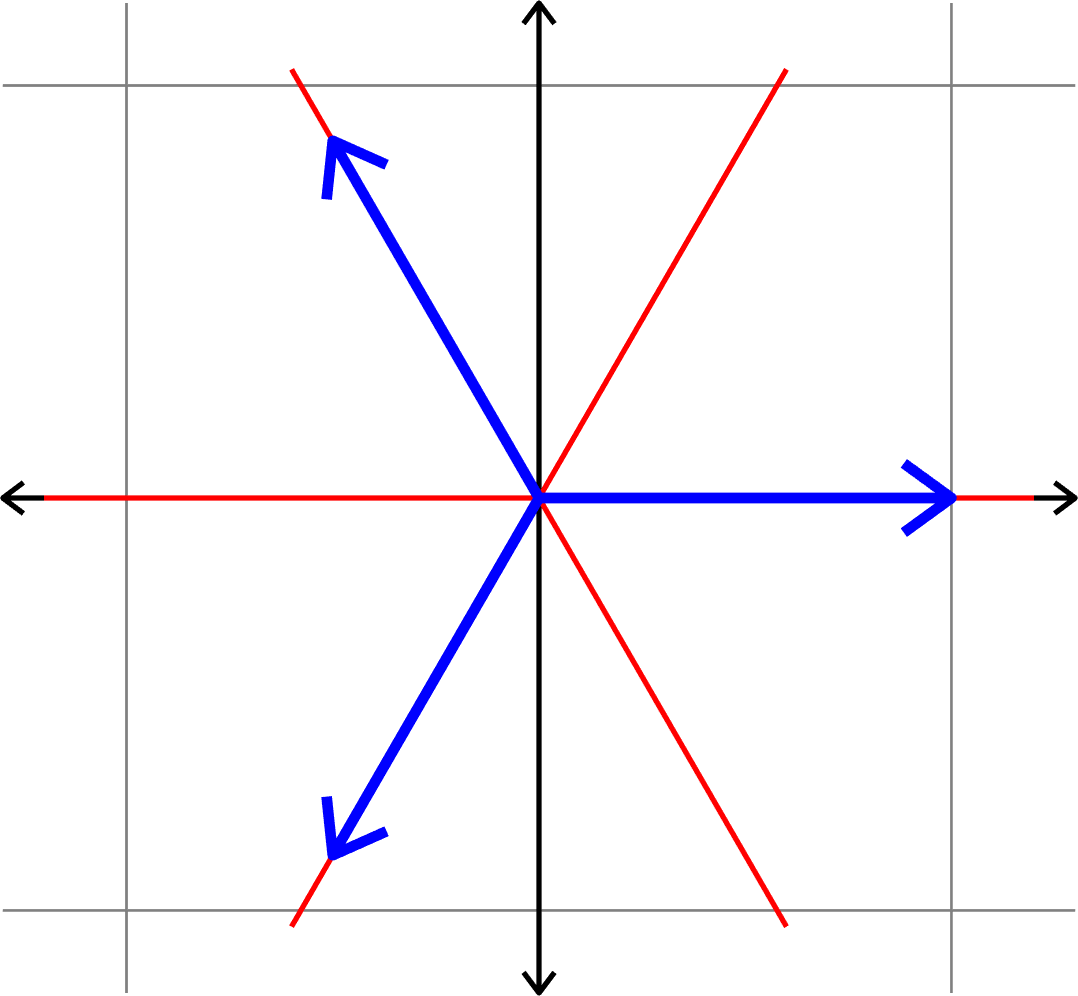
Definition. Given a collection of unit vectors \(\Phi=(\varphi_{i})_{i=1}^{N}\), we define the coherence \[\mu(\Phi) = \max_{i\neq j}|\langle \varphi_{i},\varphi_{j}\rangle|.\]
Measuring how "spread out" vectors are
\[\mu(\Phi) = \cos(\theta)\]
\(\mu(\Phi) = \cos(\theta)\)??

\(\mu(\Phi) = \cos(\theta)\)
Measuring how "spread out" vectors are
Definition. Given a collection of unit vectors \(\Phi=(\varphi_{i})_{i=1}^{N}\), we define the coherence \[\mu(\Phi) = \max_{i\neq j}|\langle \varphi_{i},\varphi_{j}\rangle|.\]
Example.
Measuring how "spread out" vectors are
Definition. Given a collection of unit vectors \(\Phi=(\varphi_{i})_{i=1}^{N}\), we define the coherence \[\mu(\Phi) = \max_{i\neq j}|\langle \varphi_{i},\varphi_{j}\rangle|.\]
Vectors that are as spread out as possible
Theorem (the Welch bound). Given a collection of unit vectors \(\Phi=(\varphi_{i})_{i=1}^{N}\) in \(\mathbb{C}^d\), the coherence satisfies
\[\mu(\Phi)\geq \sqrt{\frac{N-d}{d(N-1)}}.\]
Equality holds if and only if the following two conditions hold:
- Tight: There is a constant \(A>0\) such that \[\sum_{i=1}^{N}|\langle v,\varphi_{i}\rangle|^{2} = A\|v\|^{2} \quad\text{for all } v.\]
- Equiangular: There is a constant \(\alpha\) such that \[|\langle\varphi_{i},\varphi_{j}\rangle| = \alpha\quad\text{for all }i\neq j\]
A collection of equal norm vectors which is both equiangular and tight is known as an equiangular tight frame (ETF). These are also known as Welch bound equality codes.
Short, fat matrices
Given a collection of unit vectors \(\Phi=(\varphi_{i})_{i=1}^{N}\) in \(\mathbb{C}^d\), we will not distinguish between the sequence of vectors, and the \(d\times N\) matrix
\[\Phi = \begin{bmatrix} | & | & & |\\ \varphi_{1} & \varphi_{2} & \cdots & \varphi_{N}\\ | & | & & |\end{bmatrix}\]
Two other important matrices:
The gram matrix:
\[\Phi^{\ast}\Phi = \begin{bmatrix}\langle \varphi_{1},\varphi_{1}\rangle & \langle \varphi_{1},\varphi_{2}\rangle & \cdots & \langle \varphi_{1},\varphi_{N}\rangle\\ \langle \varphi_{2},\varphi_{1}\rangle & \langle \varphi_{2},\varphi_{2}\rangle & & \vdots\\ \vdots & & \ddots & \vdots\\ \langle \varphi_{N},\varphi_{1}\rangle & \cdots & \cdots & \langle \varphi_{N},\varphi_{N}\rangle\end{bmatrix}\]
The frame operator: \(\Phi\Phi^{\ast}\)
1. Tight:
There is a constant \(A>0\) such that \[\sum_{i=1}^{N}|\langle v,\varphi_{i}\rangle|^{2} = A\|v\|^{2} \quad\text{for all } v.\]
\(\Leftrightarrow\quad\Phi\Phi^{\ast} = AI\) (that is, the rows of \(\Phi\) are orthogonal and equal norm)
\(\Leftrightarrow\quad\Phi^{\ast}\Phi\) is a multiple of a projection.
2. Equiangular: There is a constant \(\alpha\) such that \[|\langle\varphi_{i},\varphi_{j}\rangle| = \alpha\quad\text{for all }i\neq j.\]
\(\Leftrightarrow\quad\Phi^{\ast}\Phi\) has \(1\)'s on the diagonal, and modulus \(\alpha\) entries elsewhere.
Tightness and equiangularity can be rephrased in terms of the matrix \(\Phi\):
Examples of equiangular tight frames
Example 2. Consider the (multiple of a) unitary matrix

Example 1. Consider the (multiple of a) unitary matrix
\[\left[\begin{array}{rrrr}1 & -1 & 1 & -1\\ 1 & 1 & -1 & -1\\ 1 & -1 & -1 & 1\end{array}\right]\]
\[\left[\begin{array}{rrrr} 1 & 1 & 1 & 1\\ 1 & -1 & 1 & -1\\ 1 & 1 & -1 & -1\\ 1 & -1 & -1 & 1\end{array}\right]\]
\[\left[\begin{array}{rrrr} 1 & 1 & 1\\ \sqrt{2} & -\sqrt{\frac{1}{2}} & -\sqrt{\frac{1}{2}}\\ 0 & \sqrt{\frac{3}{2}} & -\sqrt{\frac{3}{2}}\end{array}\right]\]
\[\left[\begin{array}{rrrr}\sqrt{2} & -\sqrt{\frac{1}{2}} & -\sqrt{\frac{1}{2}}\\ 0 & \sqrt{\frac{3}{2}} & -\sqrt{\frac{3}{2}}\end{array}\right]\]
Examples of equiangular tight frames
Example 3.
Part 2.
Harmonic ETFs
Using (abelian) groups to build ETFs
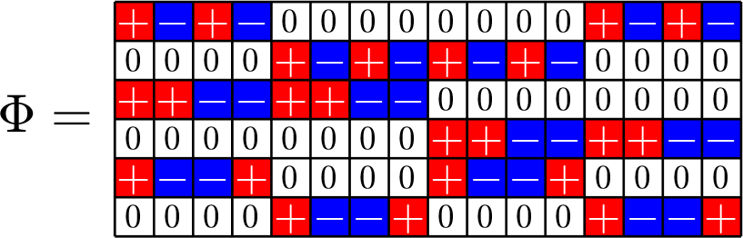
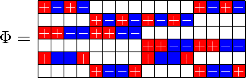
\[\Z_{7}\left\{\begin{array}{c} 0\\ 1\\ 2\\ 3\\ 4\\ 5\\ 6 \end{array}\right. \left[\begin{array}{ccccccc} 1 & 1 & 1 & 1 & 1 & 1 & 1\\ 1 & \omega & \omega^2 & \omega^3 & \omega^4 & \omega^5 & \omega^6\\ 1 & \omega^2 & \omega^4 & \omega^6 & \omega & \omega^3 & \omega^5\\ 1 & \omega^3 & \omega^6 & \omega^2 & \omega^5 & \omega & \omega^4\\ 1 & \omega^4 & \omega & \omega^5 & \omega^2 & \omega^6 & \omega^3\\ 1 & \omega^5 & \omega^3 & \omega & \omega^6 & \omega^4 & \omega^2\\ 1 & \omega^6 & \omega^5 & \omega^4 & \omega^3 & \omega^2 & \omega \end{array}\right]\]
\[\begin{array}{c} 1\\ 2\\ 4 \end{array}\left[\begin{array}{ccccccc} 1 & \omega & \omega^2 & \omega^3 & \omega^4 & \omega^5 & \omega^6\\ 1 & \omega^2 & \omega^4 & \omega^6 & \omega & \omega^3 & \omega^5\\ 1 & \omega^4 & \omega & \omega^5 & \omega^2 & \omega^6 & \omega^3 \end{array}\right]\]
Rows from a DFT
\[\Phi = \left[\begin{array}{ccccccc} 1 & \omega & \omega^2 & \omega^3 & \omega^4 & \omega^5 & \omega^6\\ 1 & \omega^2 & \omega^4 & \omega^6 & \omega & \omega^3 & \omega^5\\ 1 & \omega^4 & \omega & \omega^5 & \omega^2 & \omega^6 & \omega^3 \end{array}\right]\]
Rows from a DFT
\(\Phi\) is tight, since it is rows out of a unitary.
\(\Phi\) is equiangular, since \(D=\{1,2,4\}\subset\Z_{7}\) is a difference set.
That is, if we look at the difference table
\[\begin{array}{r|rrr} - & 1 & 2 & 4\\ \hline 1 & 0 & 6 & 4\\ 2 & 1 & 0 & 5\\ 4 & 3 & 2 & 0 \end{array}\]
every nonidentity group element shows up the same number of times
Difference sets \(\Rightarrow\) equiangular?
If \(\varphi_{j} = \left[\begin{array}{c} \omega^j\\ \omega^{2j}\\ \omega^{4j}\end{array}\right]\) for \(j=0,1,\ldots,6,\) then
Note that
\[\langle \varphi_{j}\varphi_{j}^{\ast}, \varphi_{k}\varphi_{k}^{\ast}\rangle_{\text{Fro}} = \text{tr}(\varphi_{j}\varphi_{j}^{\ast}\varphi_{k}\varphi_{k}^{\ast}) = \text{tr}(\varphi_{k}^{\ast}\varphi_{j}\varphi_{j}^{\ast}\varphi_{k}) = |\langle \varphi_{j},\varphi_{k}\rangle|^{2},\]
and
\[\varphi_{j}\varphi_{j}^{\ast} = \left[\begin{array}{c} \omega^j\\ \omega^{2j}\\ \omega^{4j}\end{array}\right]\left[\omega^{-j}\ \omega^{-2j}\ \omega^{-4j}\right] = \left[\begin{array}{ccc}1 & \omega^{6 j} & \omega^{4 j}\\ \omega^{1 j} & 1 & \omega^{5 j}\\ \omega^{3 j} & \omega^{2 j} & 1 \end{array}\right]\]
Hence, for \(j\neq k\)
\[|\langle\varphi_{j},\varphi_{k}\rangle|^{2} = \langle \varphi_{j}\varphi_{j}^{\ast}, \varphi_{k}\varphi_{k}^{\ast}\rangle_{\text{Fro}} = \text{sum}\left(\left[\begin{array}{ccc}1 & \omega^{6(j-k)} & \omega^{4(j-k)}\\ \omega^{1(j-k)} & 1 & \omega^{5(j-k)}\\ \omega^{3(j-k)} & \omega^{2(j-k)} & 1 \end{array}\right]\right)=2\]
Generating the ETF with the group
For each \(j,k\in\{0,\ldots,6\}\) set
\[\lambda_{k} = \left[\begin{array}{ccc} w^{k} & 0 & 0\\ 0 & w^{2k} & 0\\ 0 & 0 & w^{4k}\end{array}\right],\quad \varphi_{j} = \left[\begin{array}{c} \omega^j\\ \omega^{2j}\\ \omega^{4j}\end{array}\right]\]
then
\[\lambda_{k}\varphi_{j} = \varphi_{k+j}\]
and hence the ETF is \((\lambda_{k}\varphi_{0})_{k\in\Z_{7}}.\) Note that \(k\mapsto \lambda_{k}\) is a representation of the group \(\Z_{7}.\)
Theorem. Let \(G\) be a finite abelian group of order \(N.\) There is a representation \(\pi:G\to U(\mathbb{C}^{d})\) and a vector \(v\in\mathbb{C}^{d}\) such that \((\pi(g)v)_{g\in G}\) is an ETF if and only if there is an \(d\) element difference set in \(G.\)
ETFs generated in this way are called harmonic ETFs.
Part 3. Getting rid of the group I
That's not a group, that's a block design!
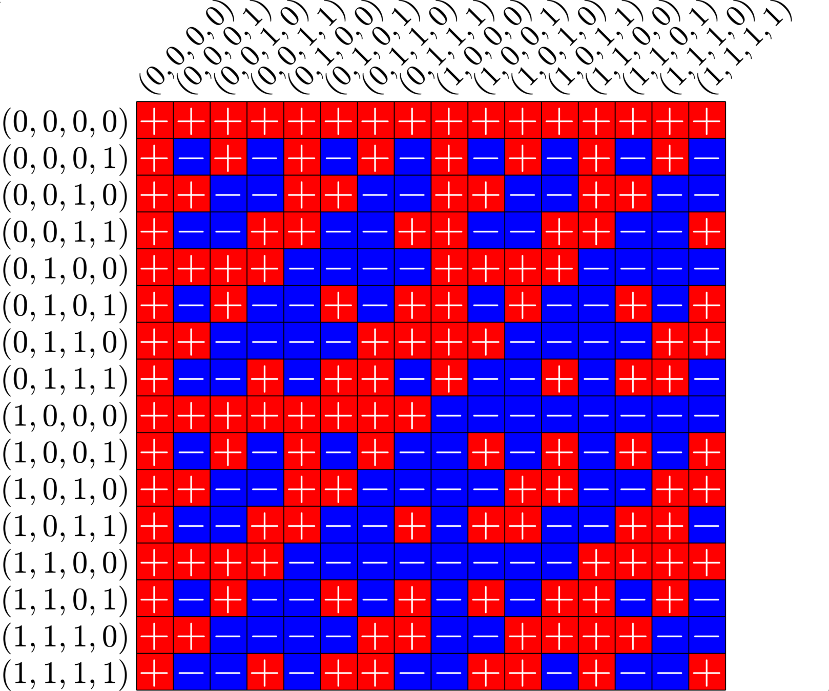
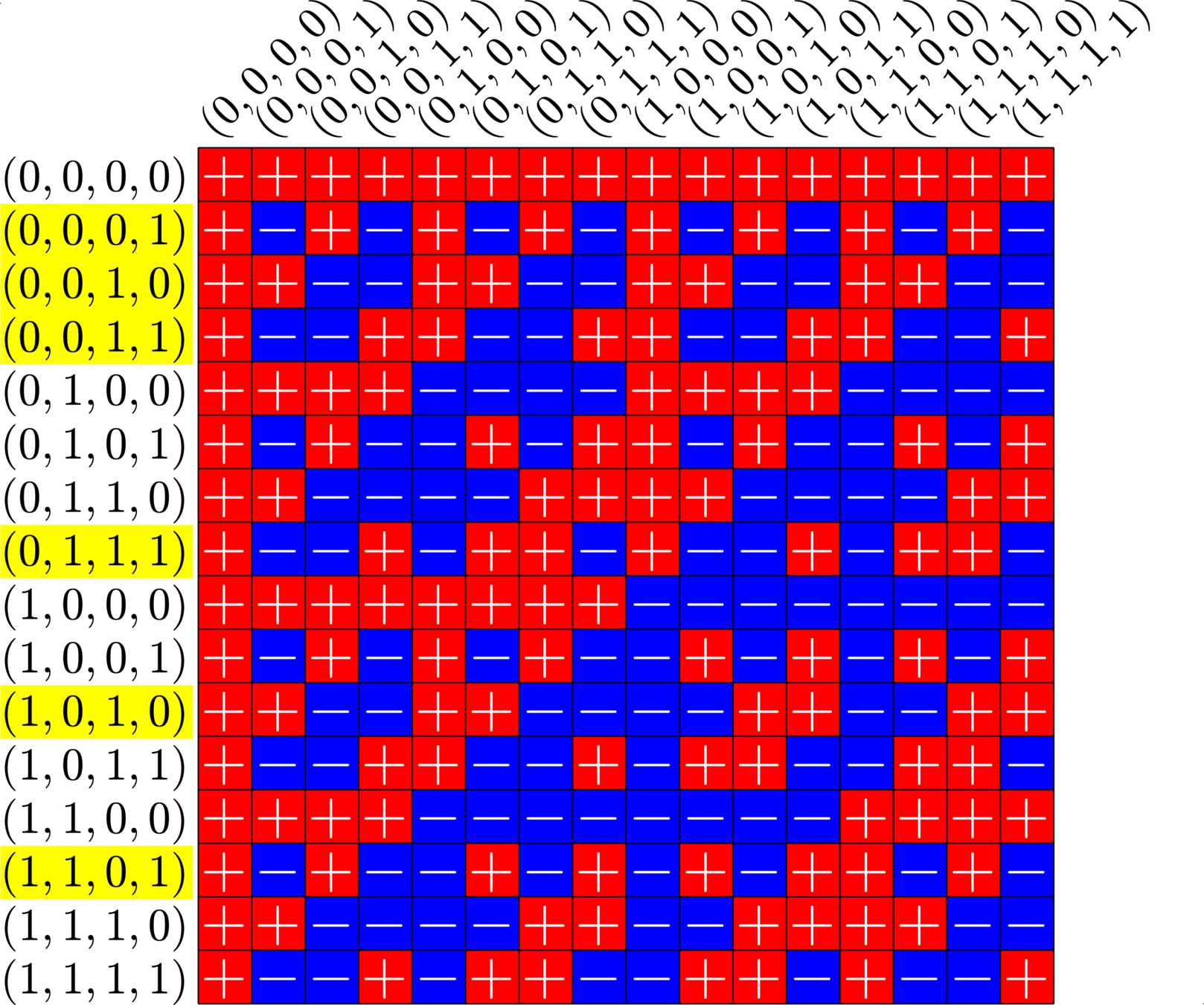
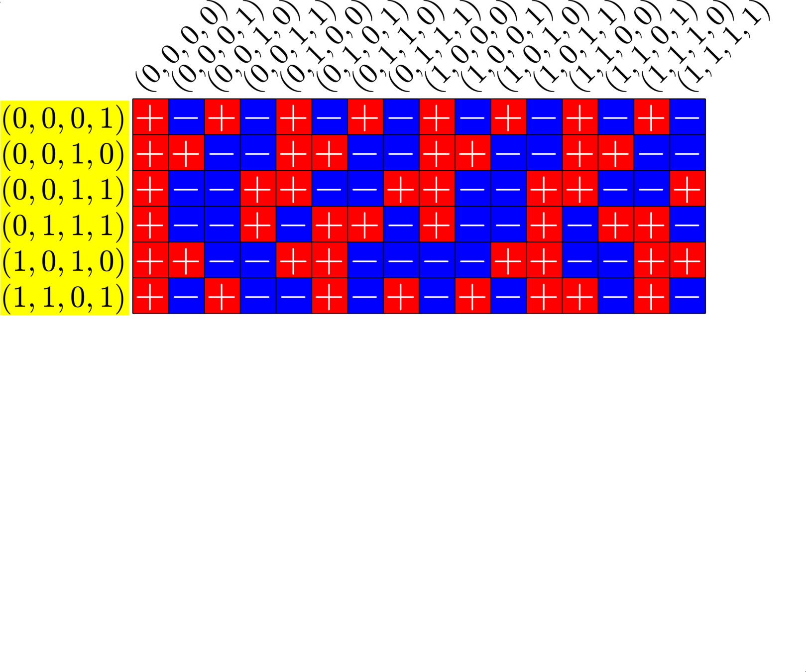
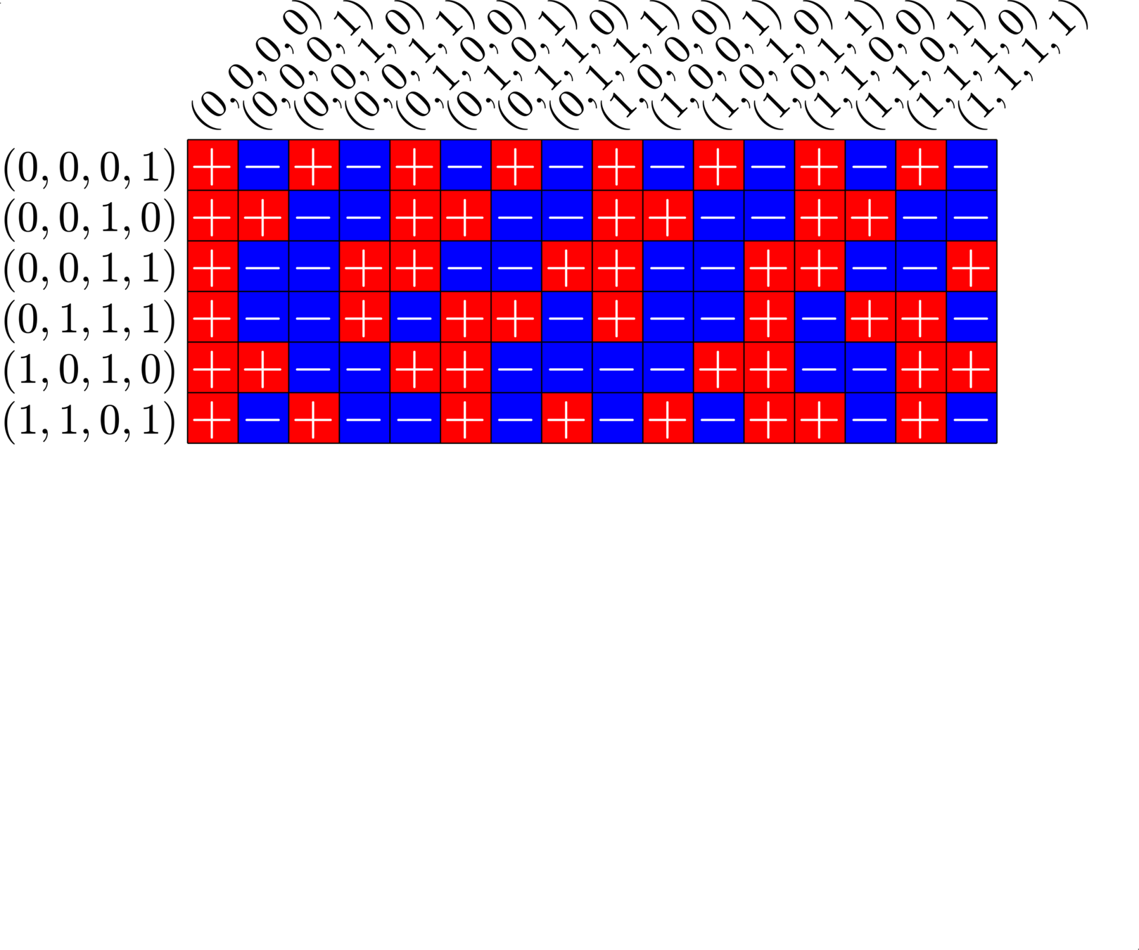
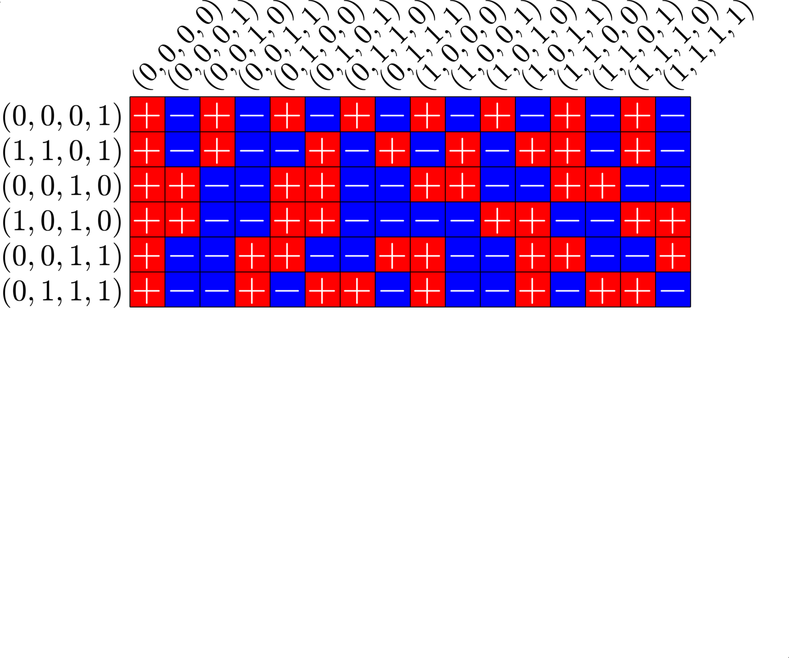
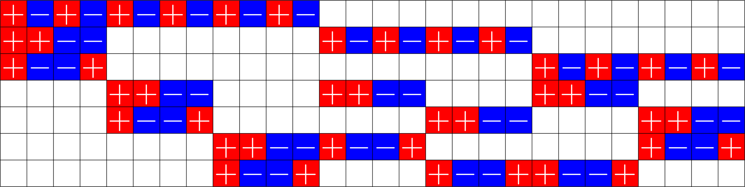
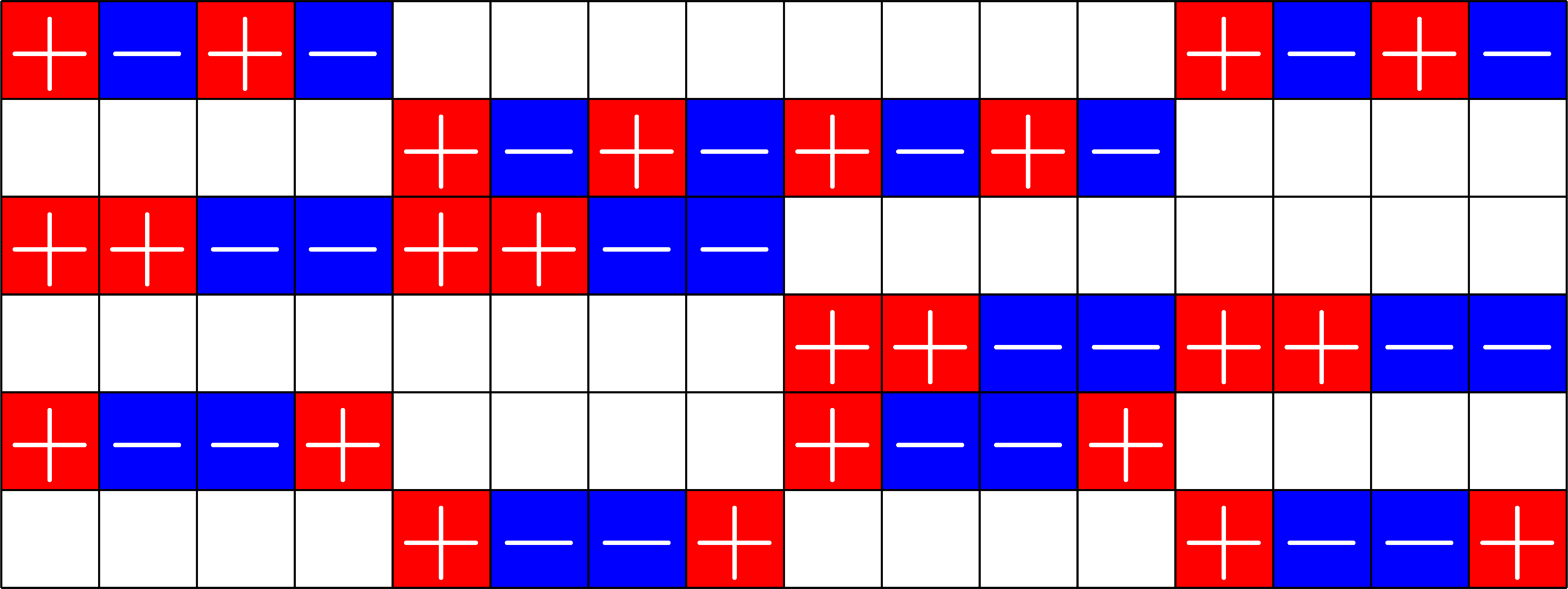
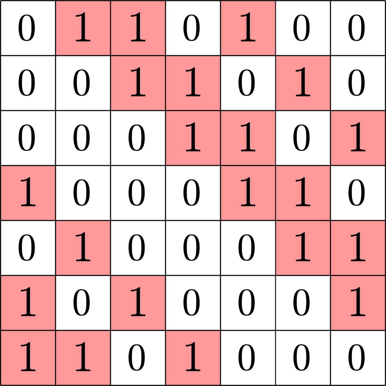
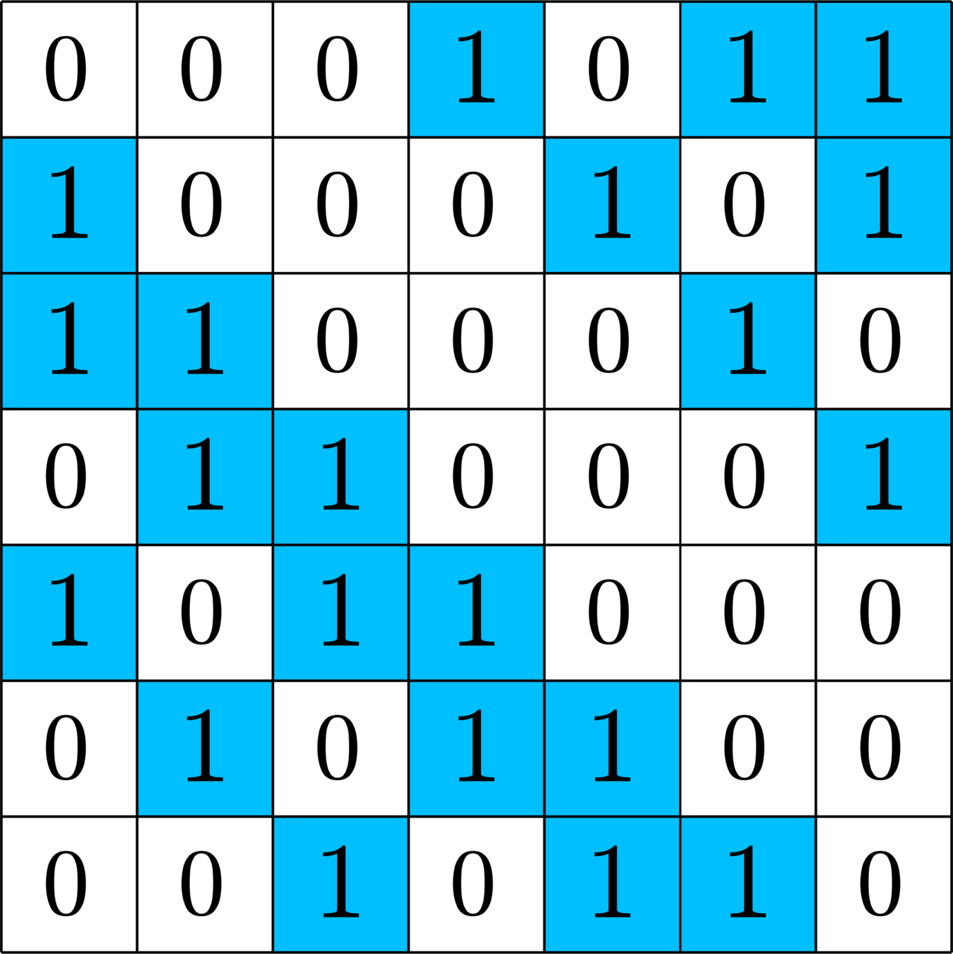
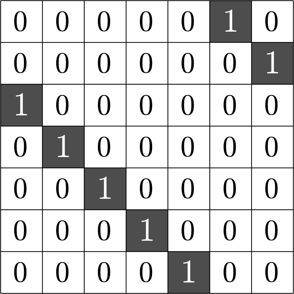
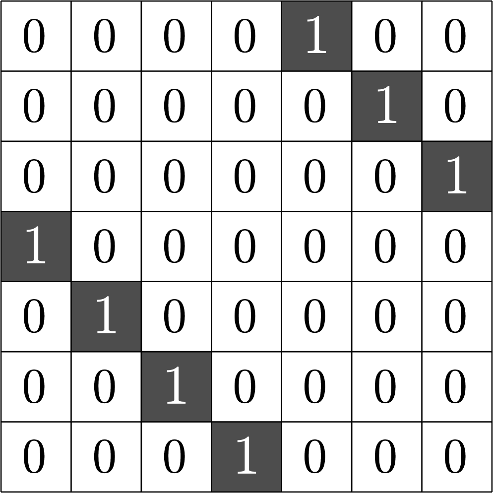
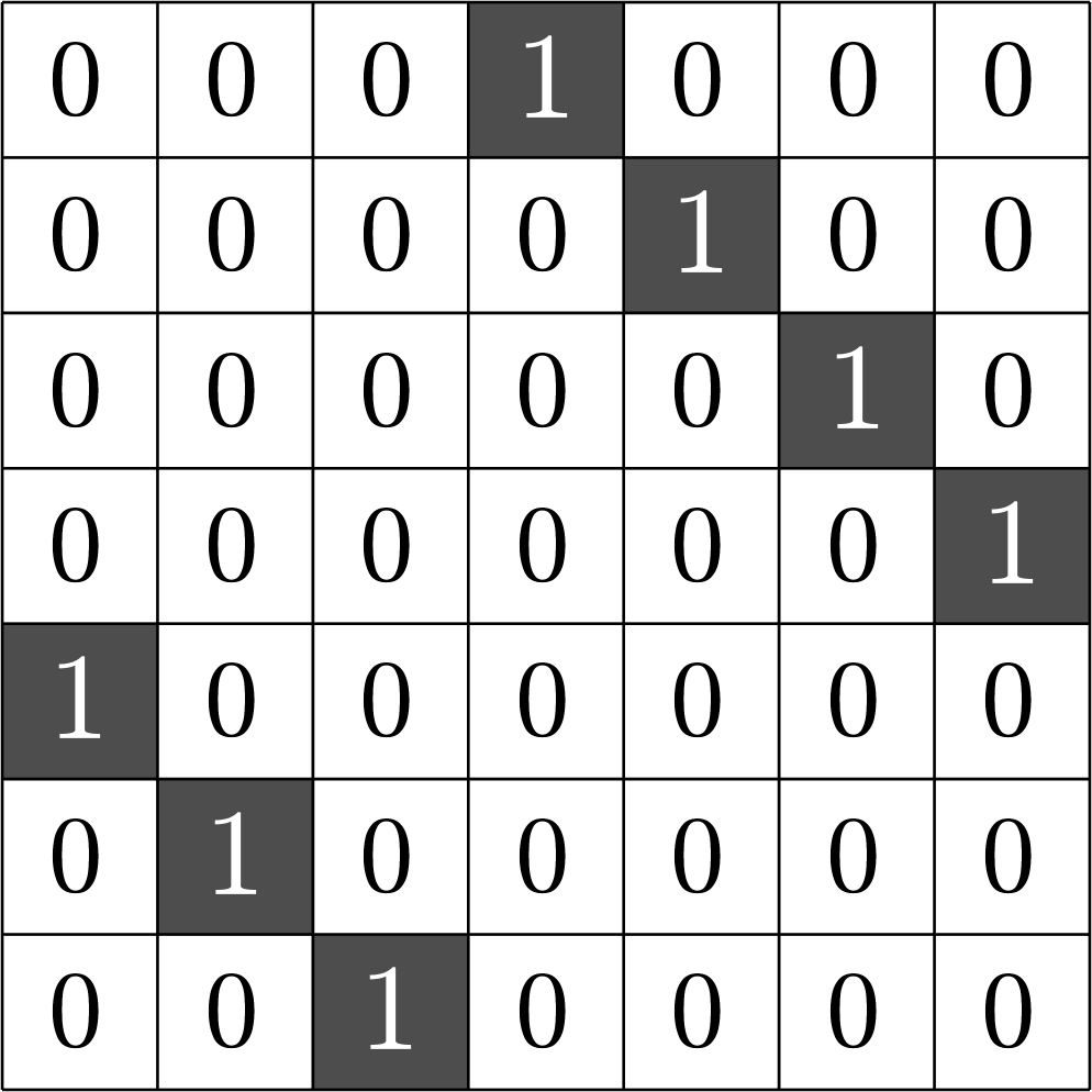
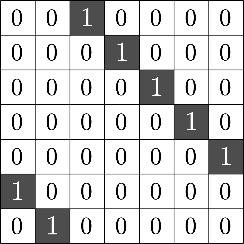
\[\begin{array}{c|cccccc} & (0,0,0,1) & (1,1,0,1) & (0,0,1,0) & (1,0,1,0) & (0,0,1,1) & (0,1,1,1)\\ \hline (0,0,0,1) & (0,0,0,0) & (1,1,0,0) & (0,0,1,1) & (1,0,1,1) & (0,0,1,0) & (0,1,1,0)\\ (1,1,0,1) & (1,1,0,0) & (0,0,0,0) & (1,1,1,1) & (0,1,1,1) & (1,1,1,0) & (1,0,1,0)\\ (0,0,1,0) & (0,0,1,1) & (1,1,1,1) & (0,0,0,0) & (1,0,0,0) & (0,0,0,1) & (0,1,0,1)\\ (1,0,1,0) & (1,0,1,1) & (0,1,1,1) & (1,0,0,0) & (0,0,0,0) & (1,0,0,1) &(1,1,0,1)\\ (0,0,1,1) & (0,0,1,0) & (1,1,1,0) & (0,0,0,1) & (1,0,0,1) & (0,0,0,0) & (0,1,0,0)\\ (0,1,1,1,) & (0,1,1,0) & (1,0,1,0) & (0,1,0,1) & (1,1,0,1) & (0,1,0,0) & (0,0,0,0) \end{array}\]
\[D=\{(0,0,0,1),(0,0,1,0),(0,0,1,1),(0,1,1,1),(1,0,1,0),(1,1,0,1)\}\]
is a (McFarland) difference set in \(G=\Z_{2}\times\Z_{2}\times\Z_{2}\times\Z_{2}\)
A McFarland difference set
The subgroup \[H=\Z_{2}\times \Z_{2}\times 0\times 0\leqslant G\] is disjoint from \(D\).
A McFarland difference set

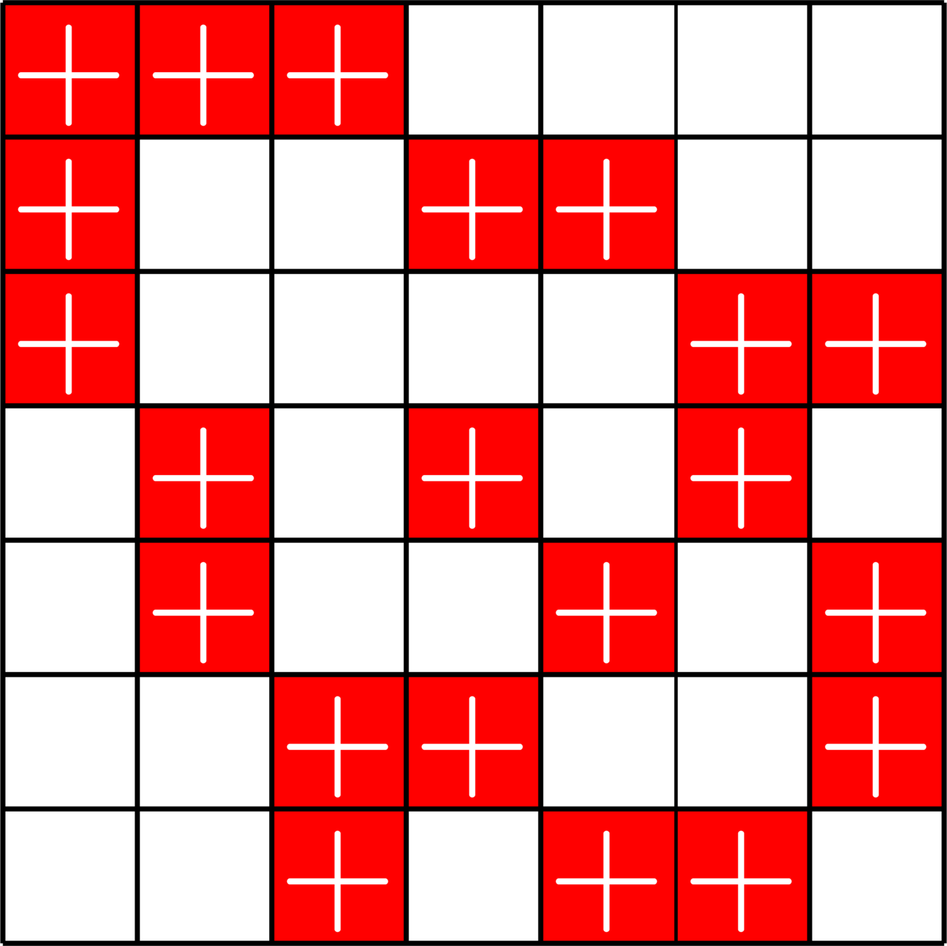
Steiner Systems
Definition. A \((2,k,v)\)-Steiner system is a \(v\) element set \(V\) together with a collection \(\mathcal{B}\) of subsets of \(V\), called blocks, with the property that each \(2\)-element subset of \(V\) is contained in exactly one block.
Example. The pair \((V,\mathcal{B})\) with
\[V = \{1,2,3,4\}\]
and
\[\mathcal{B} = \big\{\{1,4\},\{2,3\},\{1,2\},\{3,4\},\{1,3\},\{2,4\}\big\}\]
is a \((2,2,4)\)-Steiner system.
Steiner Systems
Definition. A \((2,k,v)\)-Steiner system \(\{0,1\}\)-matrix \(X\) with the following properties:
- Each row of \(X\) has exactly \(k\) ones.
- Each column of \(X\) has exactly \(r=\frac{v-1}{k-1}\) ones.
- The dot product of any distinct pair of columns is one.
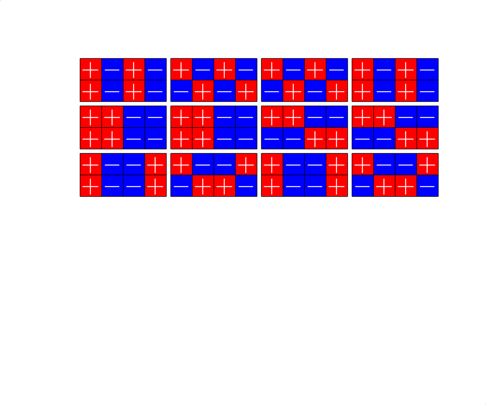
Example. The matrix
\(X = \)
is a \((2,2,4)\)-Steiner system.
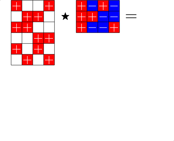
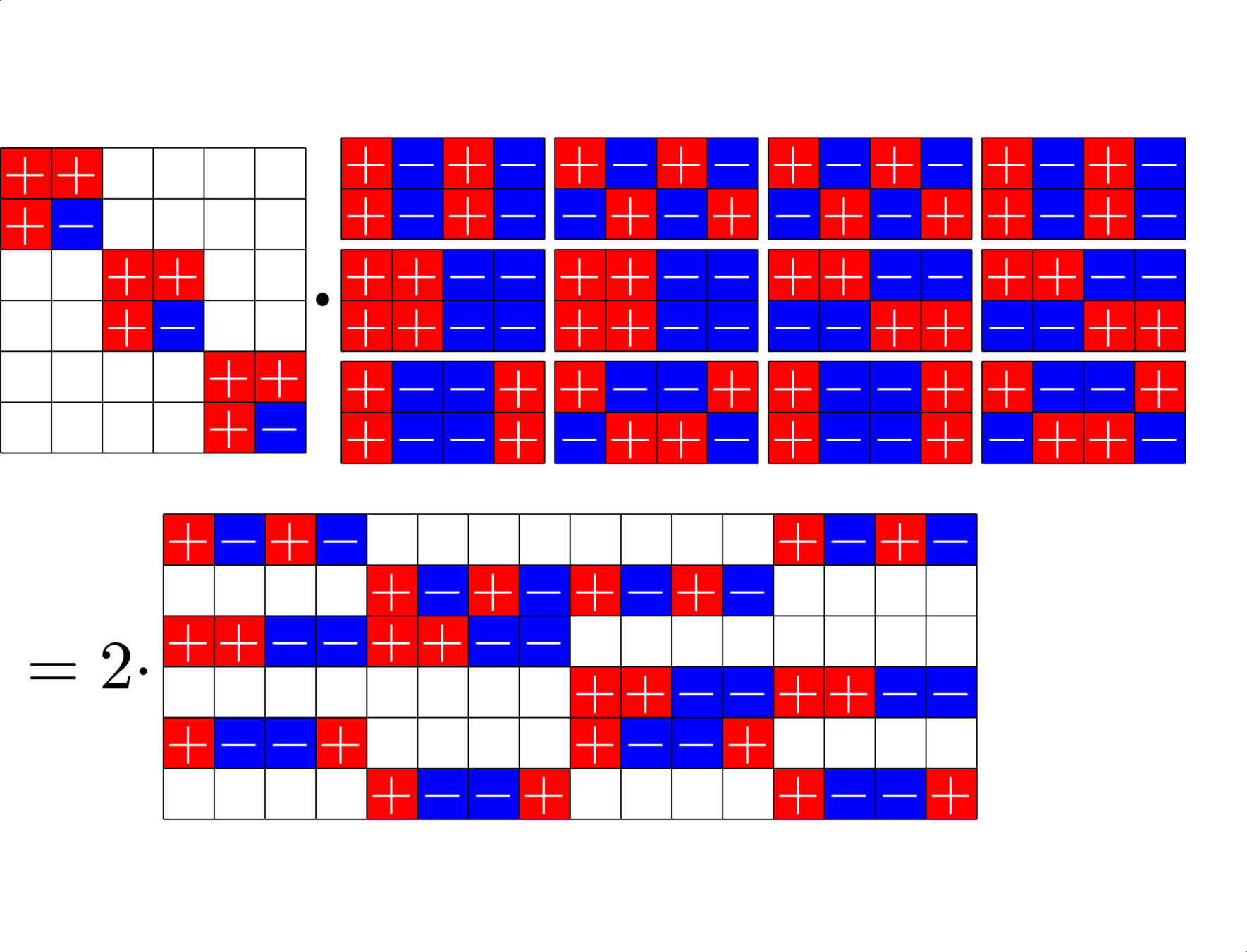
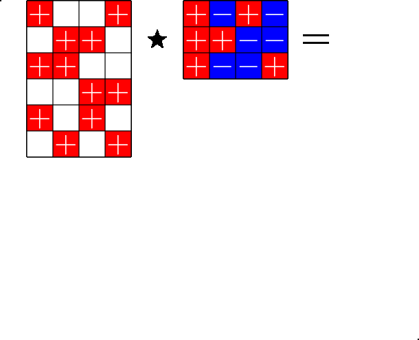
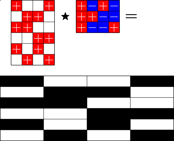
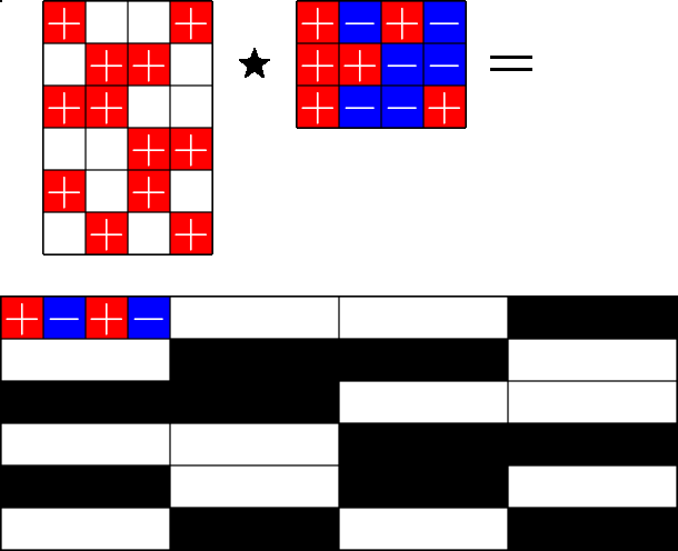
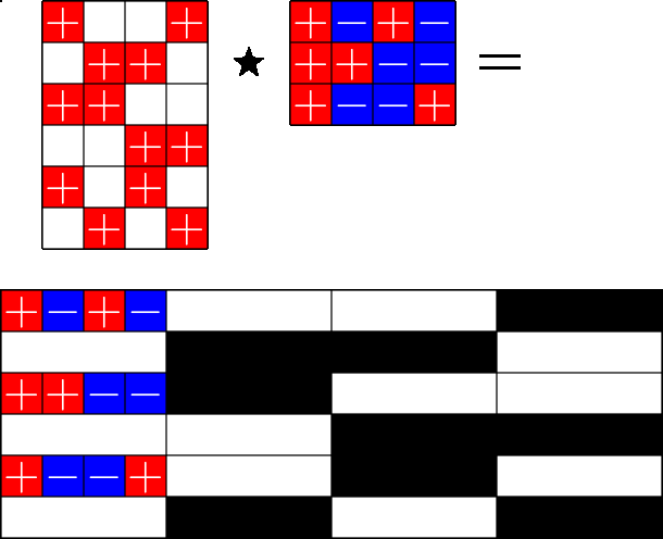
The Star Product
Steiner ETFs
(a.k.a. Generalized McFarland Difference sets)
Theorem (Fickus, Mixon, Tremain '12).
Steiner system with \(r\) ones per column
\(r\times (r+1)\) ETF with unimodular entries
\(=\)
"Steiner" ETF
An ETF that isn't harmonic

\(=\)
- There is no \(7\) element difference set in an abelian group of order \(28.\)
- But there is a \((2,3,7)\)-Steiner system


\(\bigotimes\)

\[\left[\begin{array}{l} \\ \\ \\ \\ \\ \\ \\ \\ \\ \\ \\ \end{array}\right.\]
\[\left.\begin{array}{l} \\ \\ \\ \\ \\ \\ \\ \\ \\ \\ \\ \end{array}\right]\]

\[\cong\]
Unitary transformation
\(I_{3}\otimes\)(\(2\times 3\) ETF)
\(3\times 4\) ETF with unimodular entries
???
Group Divisible Designs
Definition. A \(K\)-GDD of type \(M^{U}\) is a \(\{0,1\}\)-matrix \(X\) with the following properties:
- \(X\) has \(UM\) columns.
- Each row of \(X\) has \(K\) ones.
- \(X^{\top}X = R\cdot I_{UM}+J_{UM}-(I_{U}\otimes J_{M})\) for some \(R\in\N\)
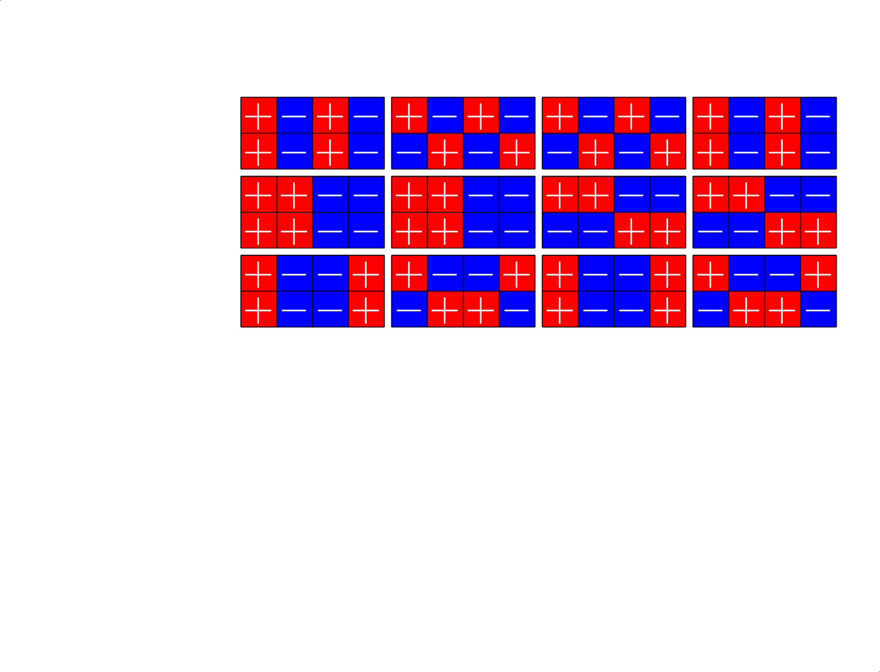
Example. The following is a \(3\)-GDD of type \(3^3\):
\(X = \)

\(X^{\top}X = \)
ETFs from GDDs
Theorem (Fickus, JJ '19). Given a
\(d\times n\) ETF
\(k\)-GDD of type \(M^{U}\)
and
provided certain integrality conditions hold, there exists a \(D\times N\) ETF with \(D>d\), \(N>n\) and \(\frac{D}{N}\approx \frac{d}{n}.\)
A New ETF
This is a \(4\)-GDD of type \(7^8\)
Combine that with a \(6\times 16\) ETF
The previous theorem produces a \(266\times 1008\) ETF, which appears to be new!
Part 4. Getting rid of the group II
Who needs groups? Association schemes can do the job!
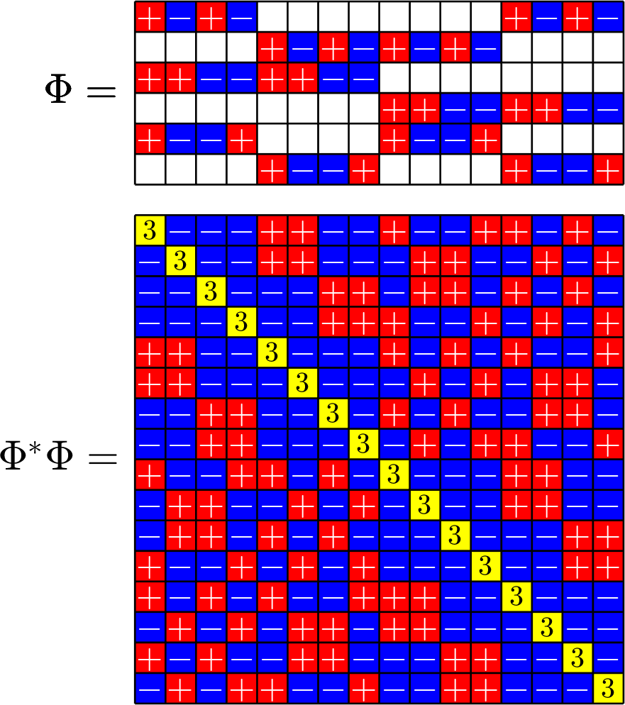
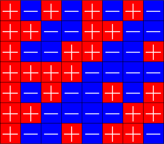
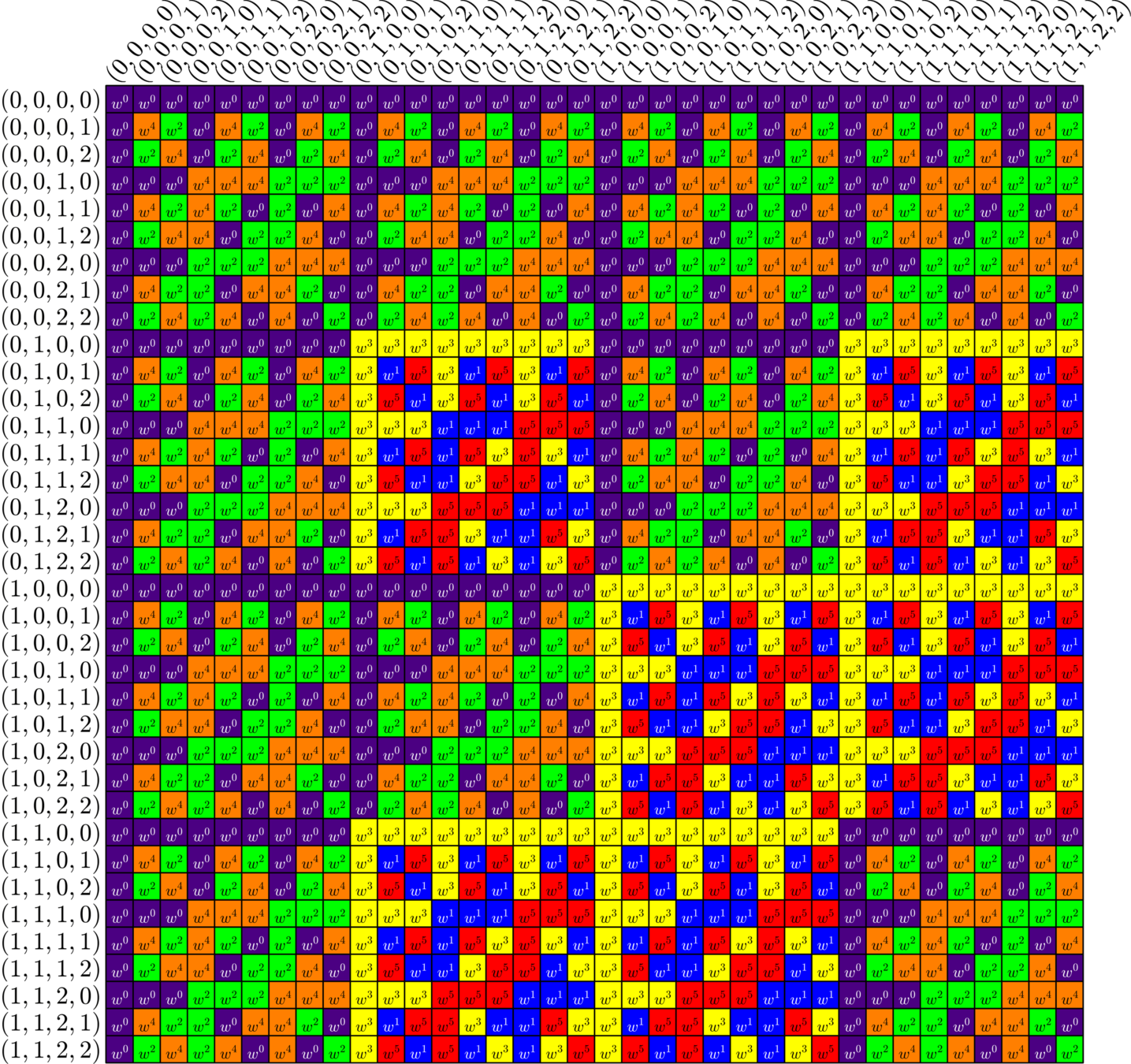
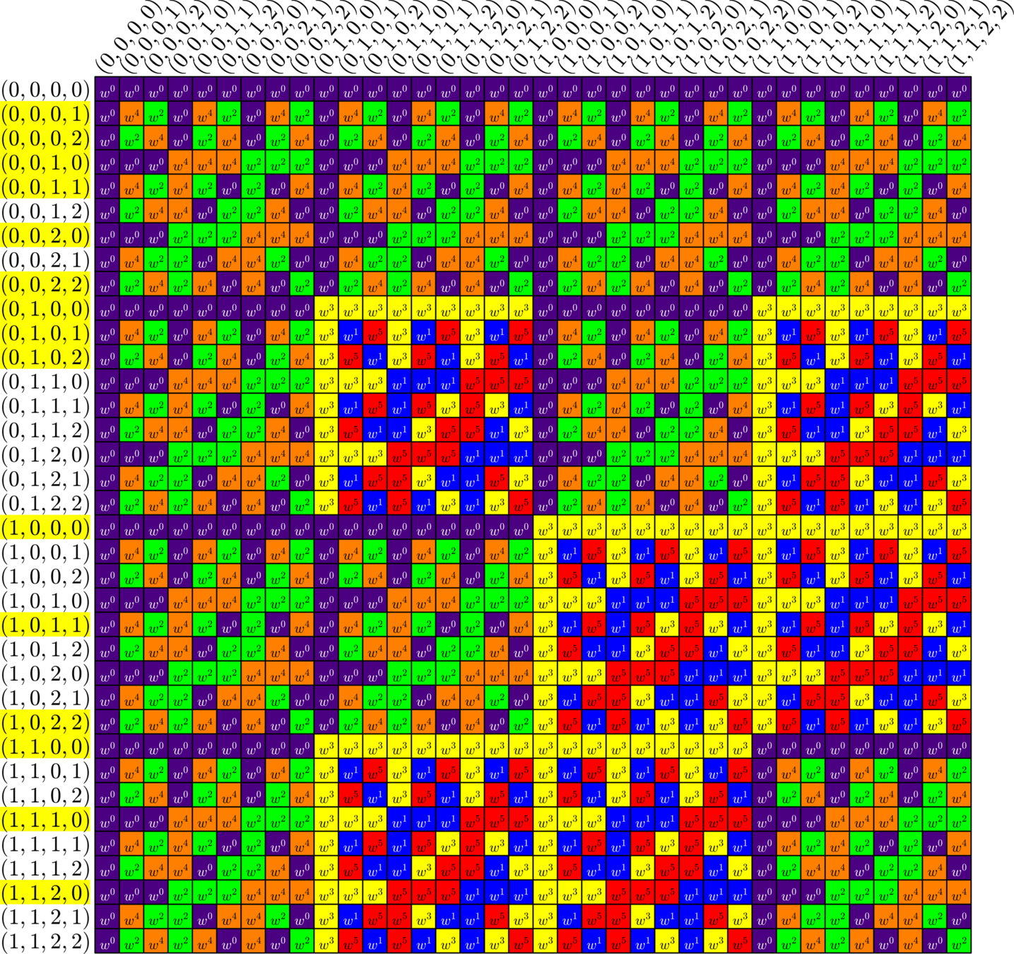
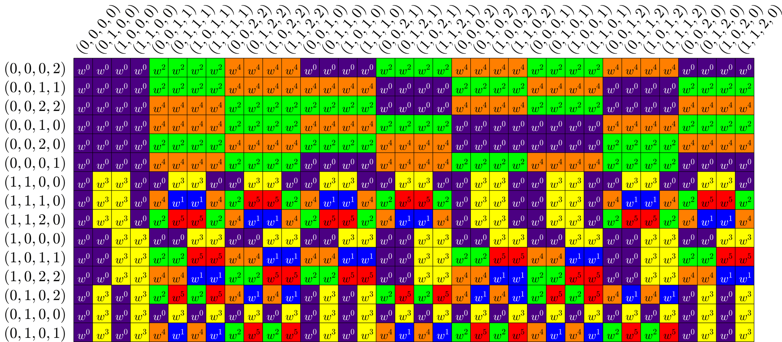
\[\Phi = \left[\begin{array}{ccccccc} 1 & \omega & \omega^2 & \omega^3 & \omega^4 & \omega^5 & \omega^6\\ 1 & \omega^2 & \omega^4 & \omega^6 & \omega & \omega^3 & \omega^5\\ 1 & \omega^4 & \omega & \omega^5 & \omega^2 & \omega^6 & \omega^3 \end{array}\right]\]
Revisiting our first harmonic ETF
\[\Phi^{\ast}\Phi = \]
\[x = \omega+\omega^2+\omega^4\qquad y=\omega^3+\omega^5+\omega^6\]
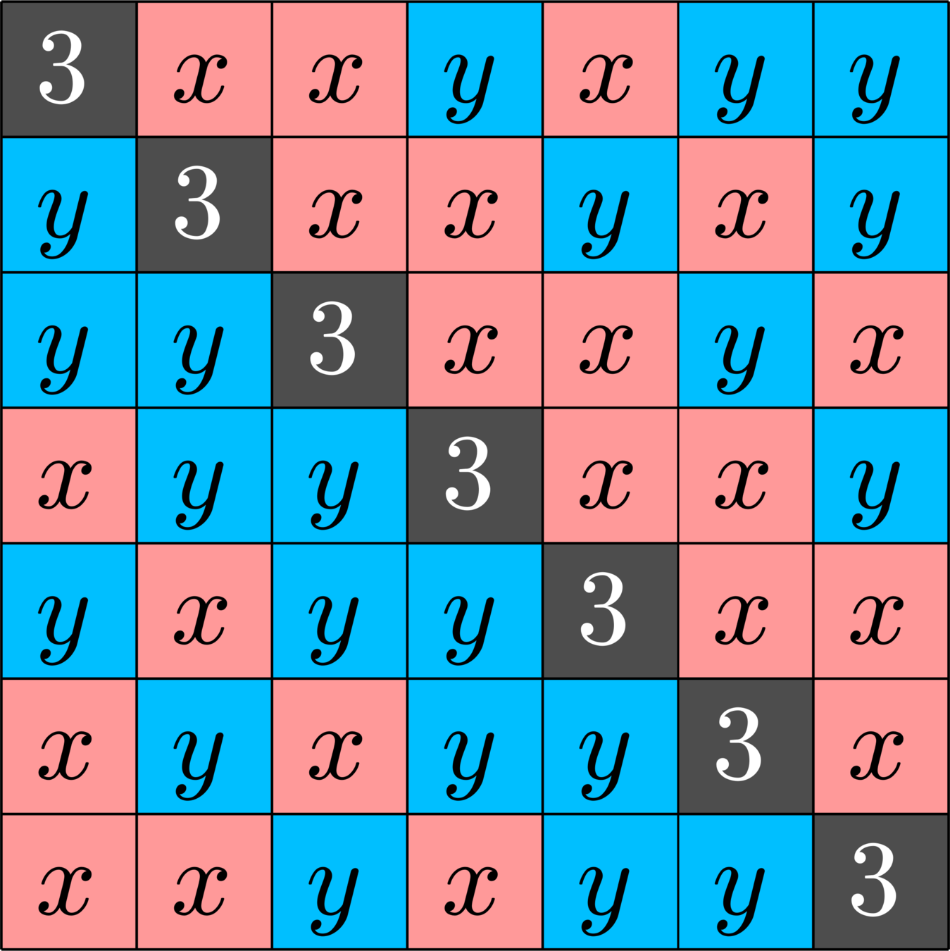
Revisiting our first harmonic ETF
\(A_{0} = \)
\(A_{1} = \)
\[\Phi^{\ast}\Phi = \]
\(A_{2} = \)
\[A_{1}A_{2} = A_{2}A_{1} = 3A_{0}+A_{1}+A_{2}\]\[A_{1}^{\top}=A_{2}\]
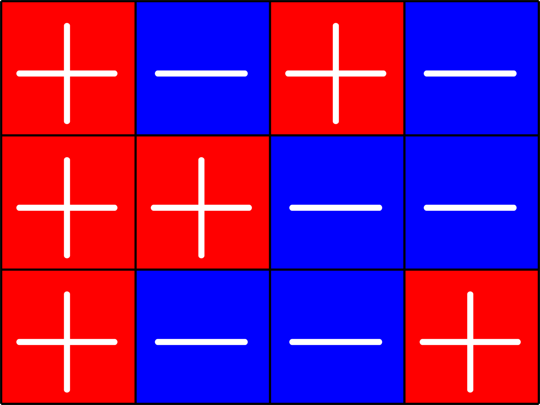
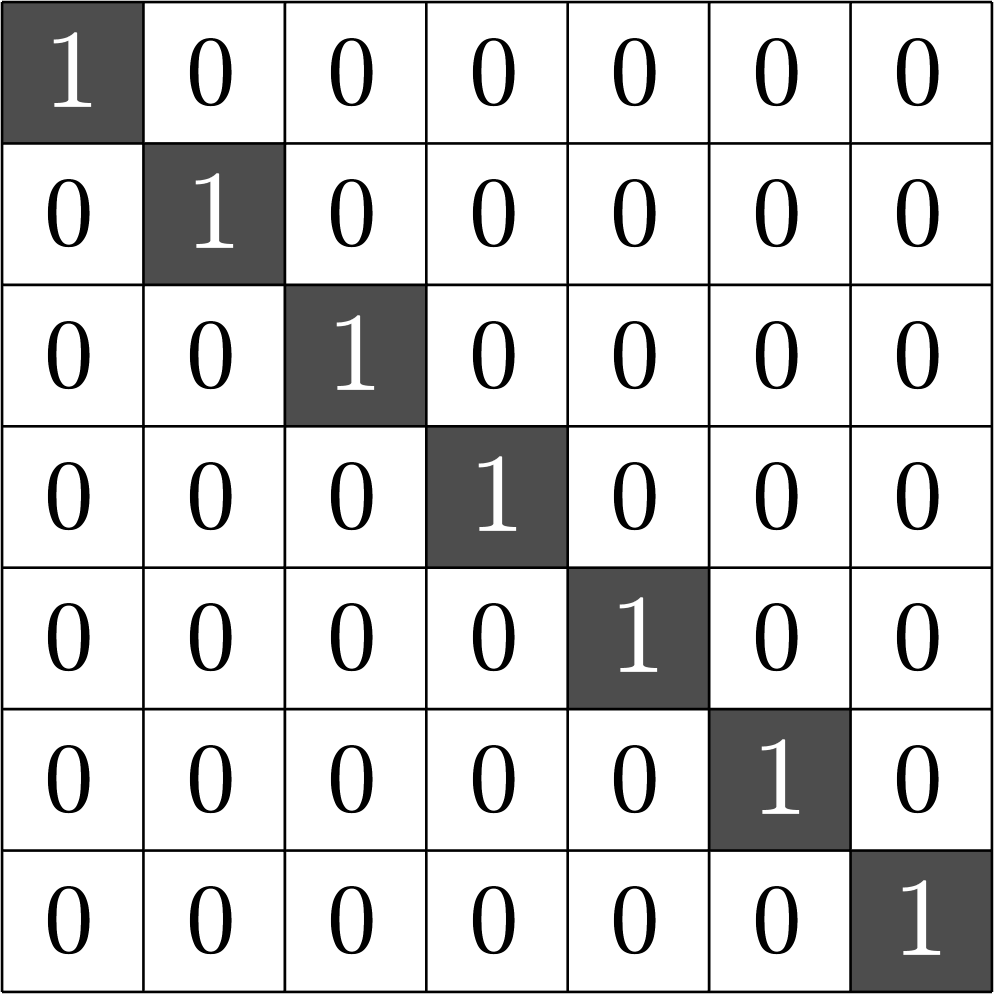
Association Schemes
Definition. A set of \(N\times N\) matrices \(X=\{A_{0},\ldots,A_{d}\}\) with entries in \(\{0,1\}\) is called an association scheme if the following three conditions hold:
- \(A_{0}=I\)
- \(A_{0}+\cdots+A_{d}=J,\) where \(J\) is the all \(1\)'s matrix
- \(\mathcal{A}=\text{span} X\) forms a commutative \(\ast\)-algebra.
Example.
\(A_{0} = \)
\(A_{1} = \)
\(A_{2} = \)
\[A_{1}A_{2} = A_{2}A_{1} = 3A_{0}+A_{1}+A_{2}\]\[A_{1}^{\top}=A_{2}\]
Abelian Groups are Association Schemes
Let \(G\) be an abelian group.
Let \((e_{g})_{g\in G}\) be an orthonormal basis for \(\mathbb{C}^{|G|}\).
For each \(g\in G\) let \(A_{g}\) be the matrix such that \(A_{g}e_{h} = e_{gh}\).
Then the collection \((A_{g})_{g\in G}\) is an association scheme.
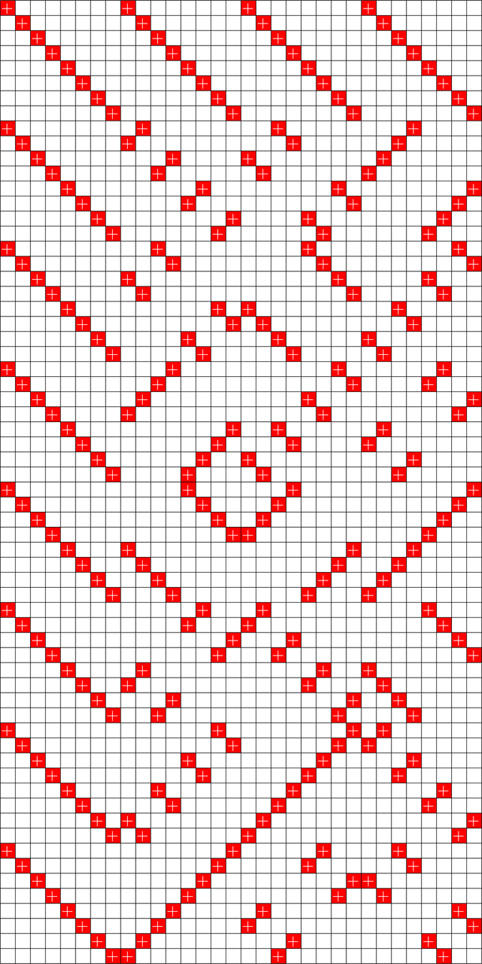
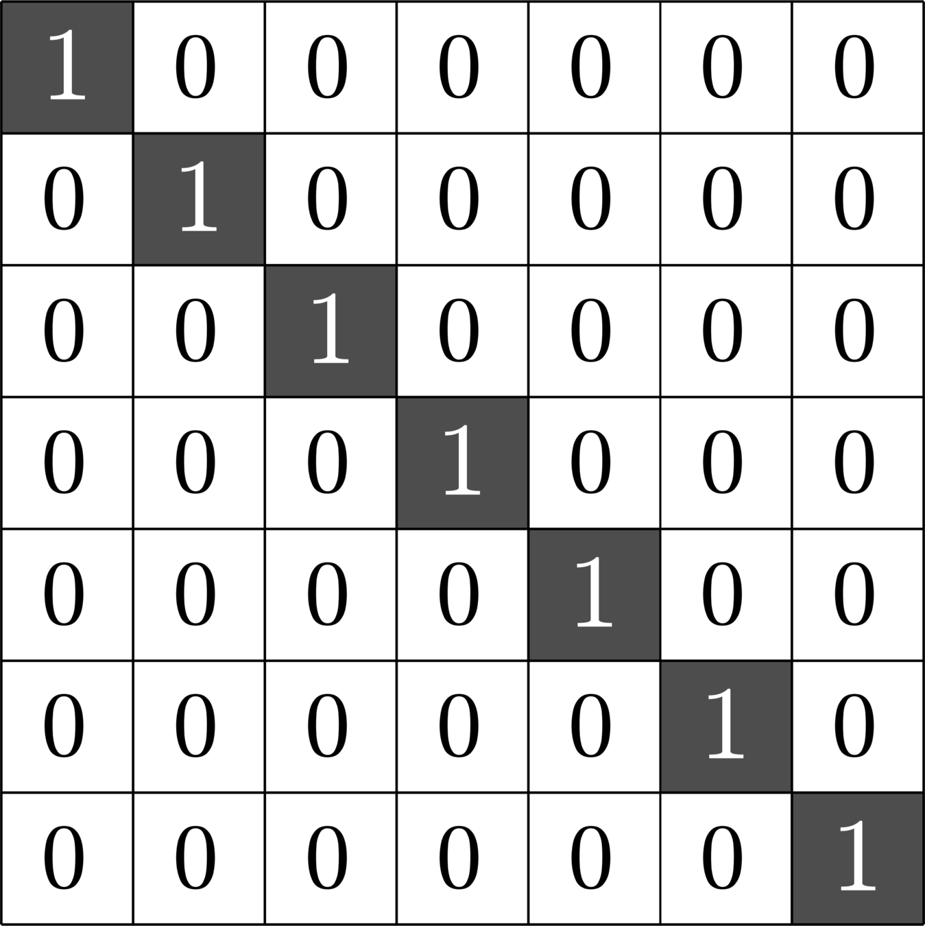
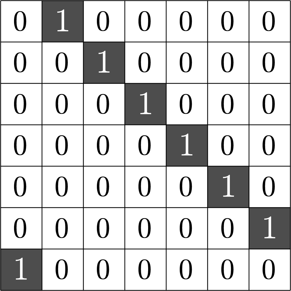
Example. The translation operators of \(\Z_{7}\) form an association scheme with \(7\) matrices:
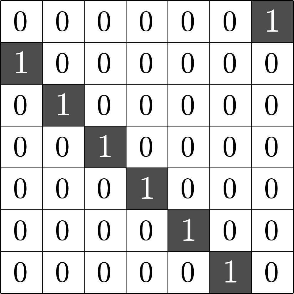
\(A_{0}=\)
\(A_{1}=\)
\(A_{2}=\)
\(A_{3}=\)
\(A_{4}=\)
\(A_{5}=\)
\(A_{6}=\)
A Generalized Dual
Let \(X = \{A_{0},A_{1},\ldots,A_{d}\}\) be an association scheme.
The matrices in \(X\) are commuting normal operators.
By the spectral theorem, there is a set of mutually orthogonal projections \[\hat{X} = \{E_{0},E_{1},\ldots,E_{d}\}\] onto the maximal eigenspaces of \(X\).
Moreover, \(\text{span}\hat{X} = \text{span} X.\)
We will refer to \(\hat{X}\) as the dual of \(X\).
Hyperdifference Sets
Definition. Let \(X\) be an association scheme with dual \(\hat{X}.\) A set \(D\subset \hat{X}\) is called a hyperdifference set if
\[\mathcal{G}_{D} := \sum_{E\in D} E\]
is the gram matrix of an ETF.
Note: For any \(D\subset \hat{X}\) the matrix \(\mathcal{G}_{D}\) is a projection. Thus we only need to check that \(\mathcal{G}_{D}\) has equal modulus off-diagonal entries.
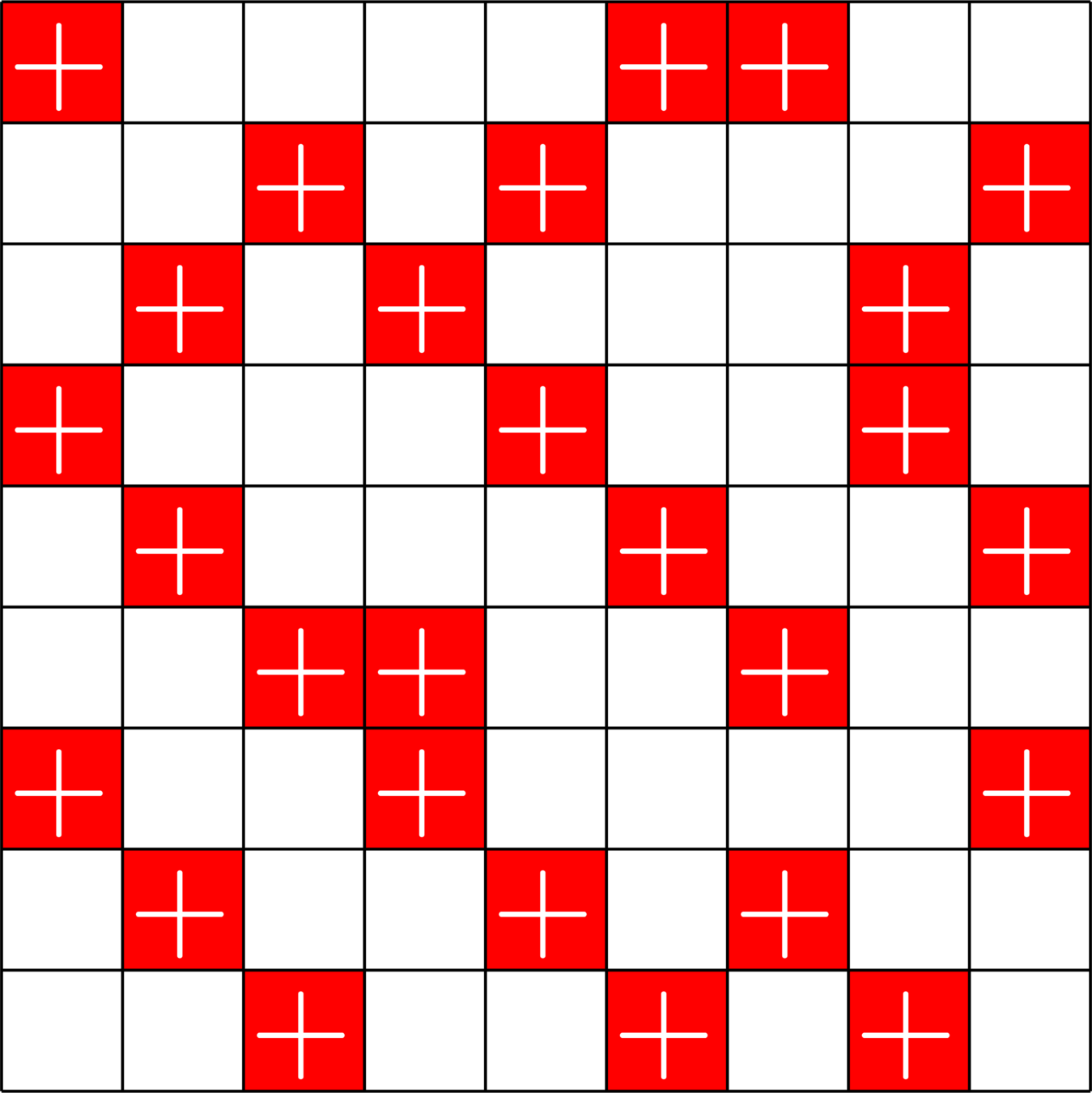
Example. Given the association scheme \(X = \{A_{0},A_{1},A_{2}\}\)
\(A_{0} = \)
\(A_{1} = \)
\(A_{2} = \)
The dual \(\hat{X} = \{E_{0},E_{1},E_{2}\}\) where
\[E_{1} = \frac{1}{7}\]
\[E_{0} = \frac{1}{7}J_{7}\]
\[E_{2} = I-E_{0}-E_{1}\]
Hence, \(D = \{E_{1}\}\) is a hyperdifference set.
Where can we look for hyperdifference sets?
Association schemes are all over the place, including:
- Abelian groups
- Schur rings over abelian groups
- Finite Gelfand pairs
- Non-abelian groups...
Definition. Let \(G=\{g_{1}=1,g_{2},\ldots,g_{N}\}\) be a group. Let \(C_{0},\ldots,C_{d}\) be the conjugacy classes of \(G\). For each \(i=0,\ldots,d\) define the \(N\times N\) matrix \(A_{i}\) by
\[A_{i}(m,n)=\begin{cases} 1 & g_{m}g_{n}^{-1}\in C_{i},\\ 0 & \text{otherwise}.\end{cases}\]
The set \(X(G) = \{A_{0},\ldots,A_{d}\}\) is called the group scheme.
Definition. Given vector spaces \(U,V\) over a field \(\mathbb{F}\) and a bilinear map \(B:U\times U\to V.\) Let \(U\times_{B} V\) be the set \(U\times V\) with multiplication
\[(u,v)\cdot(x,y) = \big(u+x,v+y+B(u,x)\big).\]
Example. Define \(B:\R^{2n}\times\R^{2n}\to\R\) by
\[B((x_{1}, y_{1}),(x_{2}, y_{2})) = x_{1}\cdot y_{2}-x_{2}\cdot y_{1},\]
then \(\R^{2n}\times_{B}\R\) is the Heisenberg group \(\mathbb{H}_{n}.\)
Theorem (Iverson, JJ, Mixon '19). For each \(k\in\N\) there is a hyperdifference set in the group \(G=\mathbb{F}_{2^{2k+1}}\times_{B}\mathbb{F}_{2^{2k+1}}\) where \(B(\alpha,\beta)=\alpha\beta^{2}.\) Moreover, the resulting ETF is generated by the action of \(G\).
A Heisenberg-ish, nonabelian group that is generating an ETF...
Shades of Zauner?
Nonabelian groups that work
Conclusions
- Actions of abelian groups give a great way to generate optimally incoherent collections of vectors, namely, ETFs.
- Harmonic ETFs are known to be rare.
- Often the necessary ingredient is actually combinatorial, that is, some \(\{0,1\}\)-matrices: Steiner systems, group divisible designs, association schemes.
- Using these allows us to go beyond abelian groups and construct a much broader class of optimal packings.
Thanks for your attention!