Flag Hilbert–Poincaré series & related zeta functions

Joshua Maglione

Otto von Guericke Universität Magdeburg

math.uni-bielefeld.de/~jmaglione

www.slides.com/joshmaglione/lincoln-lund

Creative Commons Attribution 4.0 International License

Joint with ...

Igusa's zeta functions

Count roots of \(f\in\Z[X_1,\dots, X_d]\) modulo an integer. Fix prime \(p\).

N_m(p) = \#\left\{X\in(\Z/p^m\Z)^d ~\middle|~ f(X)\equiv 0\mod p^m\right\}

Goal: understand asymptotics of

\displaystyle P_f(T) = \sum_{m=0}^\infty \dfrac{N_m(p)}{p^{dm}}T^m

Disguised \(p\)-adic integral \(Z_f(s)\) in complex variable \(s\):

P_f(p^{-s}) = \dfrac{1 - p^{-s} Z_f(s)}{1 - p^{-s}}

counting

measure

Igusa's zeta

function

Thm (Igusa 1974). Functions \(Z_f(s)\) and \(P_f(T)\) are rational in \(p^{-s}\) and \(T\), respectively.

Key step in proof: Hironaka's resolution of singularities.

Leaves open many questions:

How can we compute these?
What are the asymptotics?

Of interest to us: products of linear polynomials.

Zero locus yields a hyperplane arrangement.

Igusa zeta functions arise when computing subgroup, representation, and class-counting zeta functions.

Goal: use combinatorial & topological tools to understand asymptotics and arithmetic of the Igusa zeta function \(Z_f(s)\).

\displaystyle f(\bm{X}) = \prod_{k=1}^m L_k(\bm{X})

\deg(L_k) = 1

Bigger Picture:

\mathsf{fHP}_{\mathcal{A}}

Z_f^{\mathrm{mot}}

Z_f

\zeta_G^{\mathrm{cc}}

Z_f^{\mathrm{top}}

\mathsf{cfHP}_{\mathcal{A}}

Budur-Mustaţă-Teitler (2011)

Budur-Saito-Yuzvinsky (2011)

\left\{\phantom{\displaystyle\sum} \right.

Rossmann-Voll (2019)

van der Veer (2019)

Jensen-Kutler-Usatine (2021)

Flag Hilbert–Poincaré series

Hyperplane arrangement \(\mathcal{A}\) finite set of hyperplanes in \(K^d\).

Intersection poset: ordered by reverse inclusion

\mathcal{L}(\mathcal{A}) = \left\{\bigcap_{H\in S} H ~\middle|~ S\subseteq \mathcal{A} \right\}.

Bottom element \(\hat{0}\) : the affine space \(K^d\).

Top element \(\hat{1}\) : the common intersection (if exists).

If \(\hat{1}\in\mathcal{L}(\mathcal{A})\), then \(\mathcal{A}\) is central.

\pi_{\mathcal{A}}(Y) = \displaystyle\sum_{x\in\mathcal{L}(\mathcal{A})} \mu(\hat{0},x)(-Y)^{\mathrm{rk}(x)} = \mathrm{Poin}(\mathbb{C}^d \setminus \bigcup_{H\in\mathcal{A}}H;\; Y)

Poincaré polynomial:

\(K\!=\!\mathbb{C}\)

Coefficients are Betti numbers.

Example.

\mathsf{A}_n := \{X_i - X_j ~|~ 1 \leqslant i < j \leqslant n+1\}.

\pi_{\mathsf{A}_3}(Y) = 1 + 6Y + 11Y^2 + 6Y^3

\(\mathrm{rk}\)

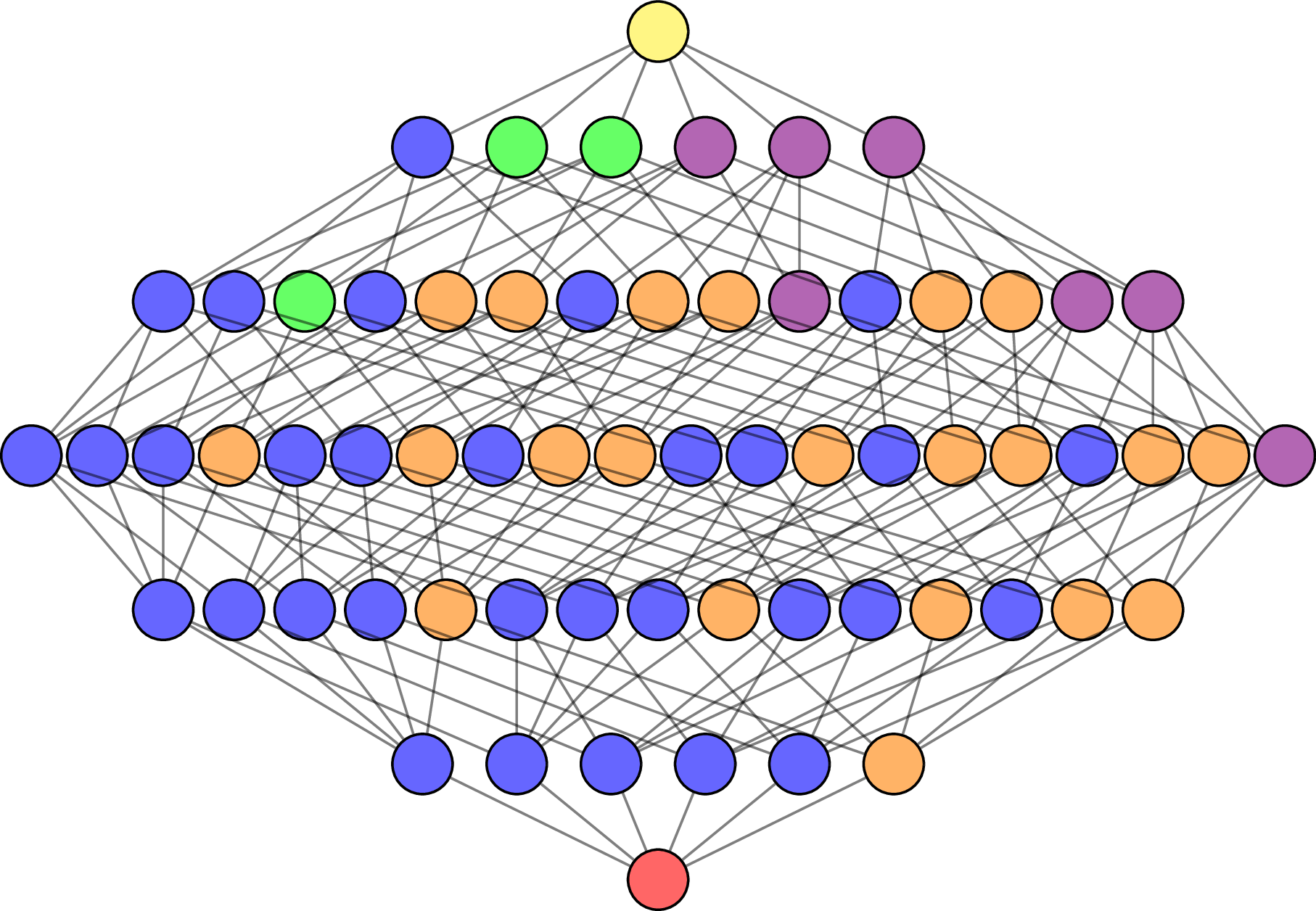
\(\mathcal{L}(\mathsf{A}_3)\)

\(\hat{0}\)

\(\hat{1}\)

\(\mathsf{A}_3\)

With \(x\in \mathcal{L}(\mathcal{A})\), two new arrangements

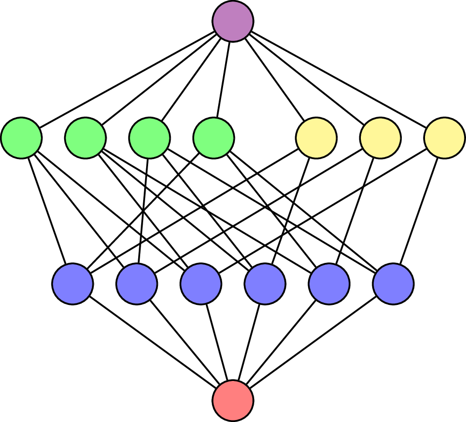
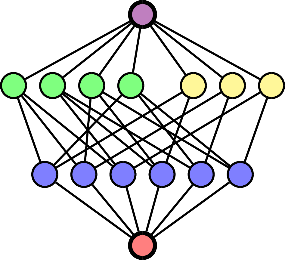
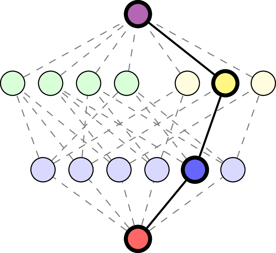
\begin{aligned} \mathcal{A}_x &= \left\{H\in\mathcal{A} ~\middle|~ x\subseteq H \right\}, & & (\text{localization})\\ \mathcal{A}^x &= \left\{x\cap H ~\middle|~ H\in\mathcal{A}\setminus\mathcal{A}_x,\; x\cap H\neq \varnothing \right\}. & & (\text{restriction}) \end{aligned}

Order complex: \(\Delta(\mathcal{L}(\mathcal{A}))\) set of flags in \(\mathcal{L}(\mathcal{A})\).

In \(\mathcal{A}_x\): \(x\) is now \(\hat{1}\). In \(\mathcal{A}^x\): \(x\) is now \(\hat{0}\).

For \(F = (x_1 < \cdots < x_\ell)\in\Delta(\mathcal{L}(\mathcal{A}))\), with \(x_0=\hat{0}\), \(x_{\ell+1}=\varnothing\),

\pi_F(Y) = \displaystyle\prod_{k=0}^{\ell} \pi_{\mathcal{A}^{x_k}_{x_{k+1}}}(Y).

Flag Poincaré polynomials.

Interval \([x_k, x_{k+1}]\)

in \(\mathcal{L}(\mathcal{A})\)

Example: \(\mathcal{A} = \mathsf{A}_3\).

\(F\) empty flag in \(\Delta(\mathcal{L}(\mathcal{A}))\):

\begin{aligned} \pi_F(Y) &= \pi_{\mathcal{A}_{\varnothing}^{\hat{0}}}(Y) = \pi_{\mathcal{A}}(Y) \\ &= 1 + 6Y + 11Y^2 + 6Y^3 \end{aligned}

For \(F = (x_1 < \cdots < x_\ell)\in\Delta(\mathcal{L}(\mathcal{A}))\), with \(x_0=\hat{0}\), \(x_{\ell+1}=\varnothing\),

\pi_F(Y) = \displaystyle\prod_{k=0}^{\ell} \pi_{\mathcal{A}^{x_k}_{x_{k+1}}}(Y).

\(F = (\quad\;)\):

\begin{aligned} \pi_F(Y) &= \pi_{\mathcal{A}^{\hat{0}}}(Y) \cdot\pi_{\mathcal{A}_{\varnothing}}(Y) \\ &= (1+Y)\cdot (1 + 3Y + 2Y^2) \end{aligned}

\begin{aligned} \pi_F(Y) &= \pi_{\mathcal{A}^{\hat{0}}}(Y) \cdot \pi_{\mathcal{A}_{\phantom{-}}}(Y) \cdot \pi_{\mathcal{A}_{\varnothing}}(Y) \\ &= (1+Y)\cdot (1 + Y) \cdot (1 + Y) \end{aligned}

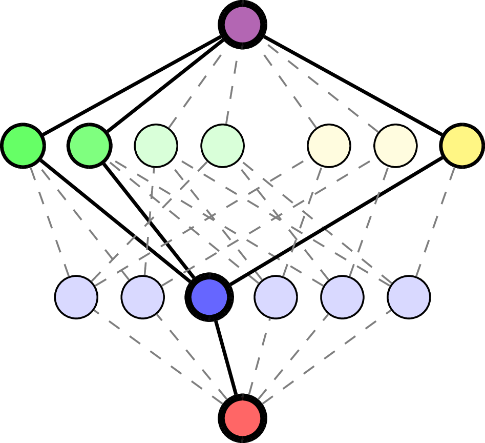
\(F = (\quad\;<\;\quad)\):

Self reciprocity

Set \(\widetilde{\mathcal{L}}(\mathcal{A}) = \mathcal{L}(\mathcal{A})\setminus\{\hat{0}\}\). The flag Hilbert–Poincaré series:

\mathsf{fHP}_{\mathcal{A}}(Y, \bm{T}) = \displaystyle\sum_{F\in\Delta(\widetilde{\mathcal{L}}(\mathcal{A}))} \pi_F(Y) \prod_{x\in F} \dfrac{T_x}{1 - T_x}

Thm (M.–Voll 2021). For \(\mathcal{A}\) defined over characteristic \(0\) field and central, then

\mathsf{fHP}_{\mathcal{A}}\left(Y^{-1},(T_x^{-1})_{x\in\widetilde{\mathcal{L}}(\mathcal{A})}\right) = (-Y)^{-\mathrm{rk}(\mathcal{A})} T_{\hat{1}} \cdot \mathsf{fHP}_{\mathcal{A}}(Y, \bm{T}).

Idea: \(\mathsf{fHP}_{\mathcal{A}}\) is equivalent to a multivariate \(p\)-adic integral.

Connections to zeta functions

Let \(K\) be a number field and \(\mathcal{O}_K\) its ring of integers.

Assume \(\mathfrak{o}\) is a compact discrete valuation ring, and

\(\mathfrak{o}\) is an \(\mathcal{O}_K\)-module,
\(\mathfrak{p}\) is its maximal ideal,
\(\mathbb{F}_q \cong \mathfrak{o}/\mathfrak{p}\).

Write \(\mathcal{A}(\mathfrak{o})\) for set of linear polynomials in \(\mathcal{O}_K[X_1,\dots, X_d]\) representing the (abstract) arrangement \(\mathcal{A}\).

Say \(\mathcal{A}(\mathfrak{o})\) has good reduction over \(\mathbb{F}_q\) if

\mathcal{L}(\mathcal{A}(\mathfrak{o})) \cong \mathcal{L}(\mathcal{A}(\mathfrak{o}/\mathfrak{p})).

is the Igusa zeta function associated to \(\mathcal{A}(\mathfrak{o})\).

\mathsf{fHP}_{\mathcal{A}}\left(-q^{-1}, (q^{-\mathrm{rk}(x) - \lambda_x s})_{x\in\widetilde{\mathcal{L}}(\mathcal{A})}\right)

Thm (M.–Voll 2021). If \(\mathcal{A}\) defined over \(K\) with good reduction over \(\mathbb{F}_q\), then

For \(x\in\mathcal{L}(\mathcal{A})\), set

\lambda_x = \# \left\{ H\in\mathcal{A} ~\middle|~ x\subseteq H \right\}.

Note: a similar multivariate substitution holds, yielding another substitution to certain class-counting zeta functions.

We see all of the candidate poles coming from combinatorial data.

\(\mathcal{L}(\mathsf{A}_3)\)

Igusa zeta function associated to

\begin{aligned} Y &= -p^{-1}, \\ T_x &= \begin{cases} p^{-1-s} & x = \phantom{-}, \\ p^{-2-2s} & x = \phantom{-}, \\ p^{-2-3s} & x = \phantom{-}, \\ p^{-3-6s} & x = \phantom{-}. \end{cases} \end{aligned}

\dfrac{(1-p^{-1})\left(1 - 5p^{-1} + 6p^{-2} + \cdots - 6p^{-4-5s} + 5p^{-5-5s} - p^{-6-5s}\right)}{(1 - p^{-1-s})^2(1 - p^{-2-3s})(1 - p^{-3-6s})}

Igusa zeta function of \(f_{\mathsf{A}_3}\): for all primes \(p\),

f_{\mathsf{A}_3}(\bm{X}) = (X_1 - X_2)(X_1 - X_3)(X_1 - X_4)(X_2 - X_3)(X_2 - X_4)(X_3 - X_4)

Class counting zeta function

\zeta^{\mathrm{cc}}_{\mathbf{G}\otimes \mathbb{Z}_p}(s) = \displaystyle \sum_{m=0}^{\infty} \# \mathrm{cc}(\mathbf{G}(\mathbb{Z}/p^m\mathbb{Z})) p^{-ms}

Let \(\mathbf{G}\) be a nilpotent group scheme of finite type over \(\mathbb{Z}\):

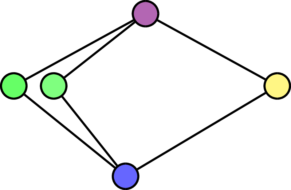
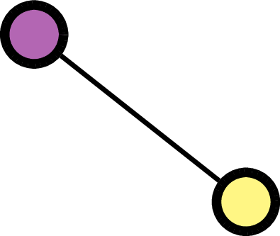
Set \(\Gamma = K_{3,2}\) and \(\mathbf{G}_{\Gamma}\) graphical group scheme.

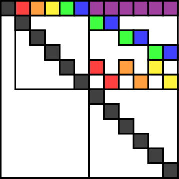
\(\mathbf{G}_{\Gamma}(\mathbb{Z}_p)\) =

\(\leqslant\mathrm{GL}_{12}(\mathbb{Z}_p)\)

\( =\langle I + E_{1,2} + E_{5,7} + E_{6,8},~\dots, \)

\( I + E_{1,6} - E_{2,8} - E_{3,10} - E_{4,12}\rangle\)

A graph \(\Gamma\) is a cograph if \(\Gamma\) contains no path on 4 vertices as an induced subgraph.

Let \(\mathcal{C}_n\) be the set of \(n\) coordinate hyperplanes in \(K^n\).

Thm (Rossmann–Voll 2019 + M.–Voll 2021). If \(\Gamma\) is a cograph on \(n\) vertices, then for all \(x\in\mathcal{L}(\mathcal{C}_{n+1})\) there exist polynomials \(f_x\) such that for all \(\mathfrak{o}\),

\zeta_{\mathbf{G}_{\Gamma}\otimes \mathfrak{o}}^{\mathrm{cc}}(s) = \mathsf{fHP}_{\mathcal{C}_{n+1}}\left(-q^{-1}, (q^{-f_x(s)})_{x\in\widetilde{\mathcal{L}}(\mathcal{C}_{n+1})} \right).

The polynomials are of the form

f_x(s) = \mu_x s + \nu_x,

for \(\mu_x\in\{0,1\}, \nu_x\in\mathbb{Z}\).

\(\mathcal{C}_n\) coordinate hyperplanes in \(K^n\) and \(\mathcal{L}(\mathcal{C}_n)\cong 2^{[n]}\).

\begin{aligned} Y &= -p^{-1}, \\ T_I &= \begin{cases} p^{6-|I|-s} & I = \phantom{-}, \\ p^{7-|I|-s} & I = \phantom{-}, \\ p^{8-|I|-s} & I = \phantom{-}, \\ p^{4-s} & I = \phantom{-}, \\ p^{-|I|} & I = \phantom{-}. \end{cases} \end{aligned}

Class counting zeta function for \(\mathbf{G}_{\Gamma}(\mathbb{Z}_p)\) for all primes \(p\):

\dfrac{1 + p^{-s} - p^{1-s} - 2p^{2-s} - p^{3-s} + p^{4-s} + p^{4-2s}}{(1-p^{3-s})(1-p^{5-s})^2}

Details: Rossmann–Voll

A different coarsening

Set each \(T_x=T\) to get coarse flag Hilbert–Poincaré series:

Easier to see examples & other combinatorial properties.

Nice form:

\mathsf{cfHP}_{\mathcal{A}}(Y, T) = \dfrac{\mathcal{N}_{\mathcal{A}}(Y, T)}{(1 - T)^{\mathrm{rk(\mathcal{A})}}}

\mathsf{cfHP}_{\mathcal{A}}(Y, T) = \displaystyle\sum_{F\in\Delta(\widetilde{\mathcal{L}}(\mathcal{A}))} \pi_F(Y) \left(\dfrac{T}{1 - T}\right)^{\# F}

\mathcal{N}_{\mathcal{A}}(Y, T) = \displaystyle\sum_{F\in\Delta(\widetilde{\mathcal{L}}(\mathcal{A}))} \pi_F(Y) T^{|F|}(1 - T)^{\mathrm{rk}(\mathcal{A})-|F|}

\mathcal{N}_{\mathsf{A}_1}(Y, T) = 1 + Y

\mathcal{N}_{\mathsf{A}_2}(Y, T) = 1 + 3Y + 2Y^2 + (2 + 3Y + Y^2)T

\begin{aligned} \mathcal{N}_{\mathsf{A}_3}(Y, T) &= 1 + 6Y + 11Y^2 + 6Y^3 \\ &\quad + (11 + 37Y + 37Y^2 + 11Y^3)T \\ &\quad + (6 + 11Y + 6Y^2 + Y^3)T^2 \end{aligned}

All nonnegative coefficients. Computed with \(\mathsf{HypIgu}\).

Braid arrangement in \(\mathbb{Q}^{n+1}\):

\mathsf{A}_n = \{X_i - X_j ~|~ 1\leqslant i < j \leqslant n+1\}

SageMath

Do coefficients of \(\mathcal{N}_{\mathcal{A}}(Y, T)\) have combinatorial interpretation?

Conjecture (M.–Voll). For arbitrary \(\mathcal{A}\), the coefficients of \(\mathcal{N}_{\mathcal{A}}(Y, T)\) are nonnegative.

\mathsf{cfHP}_{\mathcal{A}}(Y, 0) = \pi_{\mathcal{A}}(Y)

\mathsf{cfHP}_{\mathcal{A}}(0, T) = \mathrm{Hilb}(\mathbb{Q}[\Delta]; T)

where

\mathbb{Q}[\Delta] \cong \mathbb{Q}\left[Z_x ~\middle|~ x\in\widetilde{\mathcal{L}}(\mathcal{A})\right]/\left(\prod_{x\in S}Z_x ~|~ S\subseteq\widetilde{\mathcal{L}}(\mathcal{A}) \text{ not a flag}\right).

This is the Stanley–Reisner ring associated to \(\Delta(\widetilde{\mathcal{L}}(\mathcal{A}))\).

Question: Is \(\mathsf{cfHP}_{\mathcal{A}}\) the Hilbert series of an \(\mathbb{N}^2\)-graded algebra?

Coxeter arrangements

The Eulerian polynomial \(E_n(T)\) is combinatorially defined.

\begin{array}{rcccccccccc} E_1: &&&&&& 1 &&&& \\ E_2: &&&&& 1 && 1 &&& \\ E_3: &&&& 1 && 4 && 1 && \\ E_4: &&& 1 && 11 && 11 && 1 & \\ E_5: && 1 && 26 && 66 && 26 && 1 \end{array}

\mathcal{N}_{\mathcal{A}}(1, T) = \pi_{\mathcal{A}}(1) \cdot E_{\mathrm{rk}(\mathcal{A})}(T).

Thm (M.–Voll 2021). For a Coxeter arrangement \(\mathcal{A}\) with no \(\mathsf{E}_8\) factors:

Also related to numerators of Hilbert series of Stanley–Reisner rings of barycentric subdivisions of boundaries of simplexes.

Chambers of real arrangements

Assume \(K\subseteq \mathbb{R}\), so \(\mathcal{A}\) partitions \(\mathbb{R}^d\) into regions.

Say \(\mathcal{A}\) is simplicial if all chambers are simplicial cones.

\mathcal{N}_{\mathcal{A}}(1, T) \geqslant \pi_{\mathcal{A}}(1) \cdot E_{\mathrm{rk}(\mathcal{A})}(T).

Thm (Kühne–M. 2021). If \(\mathcal{A}\) is central and defined over \(\mathbb{R}\), then under coefficient-wise comparison:

Equality holds if and only if \(\mathcal{A}\) is simplicial.

Idea.

Zaslavsky's Theorem tells us that

\pi_{\mathcal{A}}(1) = \#\{\text{chambers of } \mathcal{A}\}.

\mathsf{cfHP}_{\mathcal{A}}(1, T) = \displaystyle\sum_{\mathcal{C} \text{ chamber}}\mathrm{Hilb}(R_{\mathcal{C}}; T).

where

Sum of Betti numbers of the complement of \(\mathcal{A}\) over \(\mathbb{C}\) is the number of connected components of the complement of \(\mathcal{A}\) over \(\mathbb{R}\).

This yields:

\(R_{\mathcal{C}}\) is the Stanley–Reisner ring of the barycentric subdivision of \(\partial \mathcal{C}\).

(Suggests \(\mathsf{cfHP}_{\mathcal{A}}(Y, T)\) is a "\(Y\)-twisted" version!)

Together with a deep result from Ehrenborg–Karu (2007) in algebraic combinatorics, for all chambers \(\mathcal{C}\),

h(\partial \mathcal{C}; T) \geqslant E_{\mathrm{rk}(\mathcal{A})}(T),

under coefficient-wise comparison, where

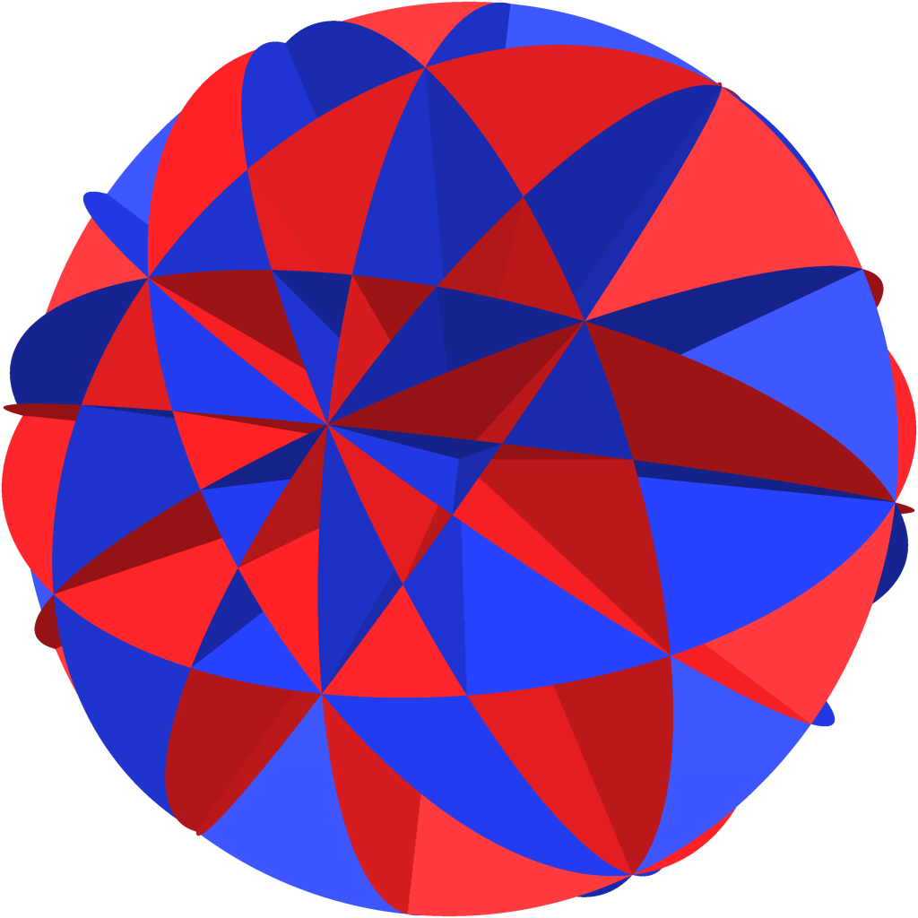
\dfrac{h(\partial \mathcal{C}; T)}{(1 - T)^{\mathrm{rk}(\mathcal{A})}} = \mathrm{Hilb}(R_{\mathcal{C}}; T).

Example. Four planes in \(\mathbb{R}^3\) in generic position.

8 cones over triangles and 6 cones over squares

\begin{aligned} \mathcal{N}_{\mathcal{A}}(1, T) &= 8(1 + 4T + T^2) + 6(1 + 6T + T^2) \\ &< 14(1 + 6T + T^2). \end{aligned}

Conjecture (Kühne–M. 2021). For \(\mathcal{A}\) of rank \(r\geqslant 3\) over arbitrary fields \(K\),

(1 + T)^{r-1} < \dfrac{\mathcal{N}_{\mathcal{A}}(1, T)}{\pi_{\mathcal{A}}(1)} < E_{\mathrm{rk}(\mathcal{A})}^{\mathsf{B}}(T).

When \(K=\mathbb{R}\), this means the average chamber of \(\mathcal{A}\) is "between" a simplicial cone and a cubical cone.

Thm (Kühne–M. 2021). The conjecture holds for \(r=3\) and \((r, K)=(4,\mathbb{R})\). If the conjecture holds, then the bounds are sharp.

Type \(\mathsf{B}\) Eulerian polynomial, \(E_r^{\mathsf{B}}(T)\), similar to type \(\mathsf{A}\).

Numerators of Stanley–Reisner rings of barycentric subdivisions of boundaries of hypercubes.

Summary

Flag Hilbert–Poincaré series shows combinatorial features of

Igusa zeta functions of products of linear polynomials,

class-counting zeta functions of nilpotent "cographical" groups.

Thm. \(\mathcal{A}\) central and characteristic \(0\) \(\implies\) \(\mathsf{fHP}_{\mathcal{A}}\) self-reciprocal.

Conj. \(\mathcal{N}_{\mathcal{A}}(Y, T)\) has nonnegative coefficients.

Thm. \(\mathcal{A}\) over \(\mathbb{R}\) and simplicial \(\implies\) \(\mathcal{N}_{\mathcal{A}}(1, T)=\pi_{\mathcal{A}}(1)\cdot E_{\mathrm{rk}(\mathcal{A})}(T)\).