A Tensor Playground:

a demonstration of $\textsf{TensorSpace}$

Joshua Maglione

jmaglione@math.uni-bielefeld.de

Universität Bielefeld

Creative Commons Attribution 4.0 International License

Began in 2015 and is still evolving.

Joint with Pete Brooksbank and James Wilson.

Funded in part by NSF: DMS-1620454.

$\textsf{TensorSpace}$ refers to a collection of Magma packages:

TensorSpace: data structures for tensors,
Sylver: algorithms for simultaneous Sylvester equations,
Densor: algorithms to construct linear closures of tensor spaces.

Constructing Tensors in $\textsf{TensorSpace}$

Flexible data structure for tensors

Goal: Want flexible definition for tensors.

Questions: Is a tensor more than just...

a high-dimensional grid?
a multilinear map?

How do the questions we want to answer motivate a data structure?

Examples require context

1. $b$ bilinear form of $V$ . Interpret:

$\langle b | : V \times V \rightarrowtail K$

3. $V$ an $A$ -module. Interpret:

$\langle \mu | : V \times A \rightarrowtail V$

2. $\psi$ an entangled system of qubits. Interpret:

$\langle \psi | : \mathbb{C}^2\times \cdots \times \mathbb{C}^2 \rightarrowtail \mathbb{C}$

Tensors in $\textsf{TensorSpace}$ are framed

We require tensors to have three things:

1. frame: $(U_0, \ldots, U_n)$ ,

2. function: $U_n\times \cdots \times U_1\rightarrowtail U_0$ ,

3. category*.

*We do not specify now, but we will come back to this.

A "default" category is assigned when not given.

Constructing a tensor from scratch

We construct the tensor

$\begin{aligned} t : \text{M}_2(\mathbb{Q}) \times \text{M}_2(\mathbb{Q}) &\rightarrowtail \text{M}_2(\mathbb{Q}),\\ (A, B) &\mapsto AB \end{aligned}$

We have two structures we define:

frame: $(\text{M}_2(\mathbb{Q}),\; \text{M}_2(\mathbb{Q}),\; \text{M}_2(\mathbb{Q}))$ ,
function: $(A, B)\mapsto AB$ .

Q := Rationals();           
A := MatrixAlgebra(Q, 2);              // 2 x 2 matrices over Q
frame := [A, A, A]; 
frame;

[
Full Matrix Algebra of degree 2 over Rational Field,
Full Matrix Algebra of degree 2 over Rational Field,
Full Matrix Algebra of degree 2 over Rational Field
]

First we define our frame.

Require a function to map a tuple of matrices to their product.

mult := func< x | x[1]*x[2] >;         // <A, B> |-> A*B
t := Tensor(frame, mult);
t;

Tensor of valence 3, U2 x U1 >-> U0
U2 : Full Vector space of degree 4 over Rational Field
U1 : Full Vector space of degree 4 over Rational Field
U0 : Full Vector space of degree 4 over Rational Field

Tensors as multilinear functions

Let's do a brief sanity check, and verify $t$ does what we expect.

X := A![2, 2/5, 0, -1];               // define matrices
Y := A![0, -3, 5, 7];                 // from sequences 
X, Y;

[  2 2/5]
[  0  -1]

[ 0 -3]
[ 5  7]

X*Y, <X, Y> @ t;

[    2 -16/5]
[   -5    -7]

(    2 -16/5    -5    -7)

Recall, the print statement for $t$ : no matrix algebras

t;

Tensor of valence 3, U2 x U1 >-> U0
U2 : Full Vector space of degree 4 over Rational Field
U1 : Full Vector space of degree 4 over Rational Field
U0 : Full Vector space of degree 4 over Rational Field

It states vector spaces, but we gave it matrices: $X$ and $Y$ .

The frame gives context, so that we leave the typing to the machines.

<X, [0, -3, 5, 7]> @ t;
<0, [1, 1, 1, 1]> @ t;

(    2 -16/5    -5    -7)
(0 0 0 0)

Structure constants

We define a tensor of the form

$\langle t| : K^{d_n} \times \cdots \times K^{d_1} \rightarrowtail K^{d_0}$

by $d_0\cdots d_n$ elements in $K$ : a $(d_n\times \cdots \times d_0)$ -grid

$[t_{i_n\cdots i_1}^{i_0}].$

Notational challenge to do this for general $n$ . We do $n=2$ :

$(u, v)\mapsto \left( \sum_{i=1}^{d_2}\sum_{j=1}^{d_1} u_{i}t_{ij}^{1} v_{j}, \ldots, \sum_{i=1}^{d_2}\sum_{j=1}^{d_1} u_{i}t_{ij}^{d_0} v_{j}\right)\in K^{d_0}.$

Let's construct an example.

d := [3, 2, 5, 4];                 // dimensions of frame
grid := [1..3*2*5*4];              // ints 1, ..., 120
t := Tensor(Q, d, grid);
t;

Tensor of valence 4, U3 x U2 x U1 >-> U0
U3 : Full Vector space of degree 3 over Rational Field
U2 : Full Vector space of degree 2 over Rational Field
U1 : Full Vector space of degree 5 over Rational Field
U0 : Full Vector space of degree 4 over Rational Field

We verify that the structure constants of $t$ are what we expect.

StructureConstants(t)[1..10];       // Only first 10 entries

[ 1, 2, 3, 4, 5, 6, 7, 8, 9, 10 ]

Notice: structure constants are a flat sequence.

The grid model provides easier understanding of data manipulation.

We describe 2 operations that potentially change the frame.

Slicing

Recall, our current tensor has the frame:

$\langle t | : \mathbb{Q}^3 \times \mathbb{Q}^2 \times \mathbb{Q}^5 \rightarrow \mathbb{Q}^4$

We grab any entry of the grid $[t_{i_n\cdots i_1}^{i_0}]$ and consider the corresponding sub-grid.

This can be interpreted as a tensor itself.

We query for the $t_{3,2,5}^{4}$ constant:

ind := [{3}, {2}, {5}, {4}];                  // last entry
Slice(t, ind);

[ 120 ]

We can query any sequence of indices.

indices := [{1, 3}, {2}, {1, 3, 4}, {4}];     // 2*1*3*1 entries
Slice(t, indices);

[ 24, 32, 36, 104, 112, 116 ]

The above example can be interpreted as a new tensor

$\langle s | : \mathbb{Q}^2 \times \mathbb{Q} \times \mathbb{Q}^3 \rightarrowtail \mathbb{Q}.$

So it might be helpful to interpret the output as a matrix.

SliceAsMatrices(t, indices, 3, 1);

[
    [ 24  32  36]
    [104 112 116]
]

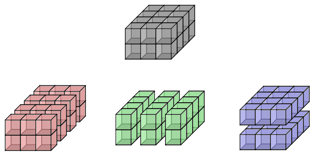
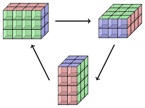
Shuffling

We apply permutations to the frame. Suppose we are framed by vector spaces

$\langle t | : U_n \times \cdots \times U_1\rightarrowtail U_0.$

For a permutation $\sigma$ of $\{0, \ldots, n\}$ , a $\sigma$ -shuffle of $t$ is a tensor

\langle \sigma(t) | : U_{\sigma(n)} \times \cdots \times U_{\sigma(1)} \rightarrowtail U_{\sigma(0)}.

Note: shuffling requires dual-spaces. $\textsf{TensorSpace}$ handles this.

We continue with current example:

\langle t | : \mathbb{Q}^3 \times \mathbb{Q}^2 \times \mathbb{Q}^5 \rightarrowtail \mathbb{Q}^4.

We apply the permutation $\sigma = (0, 2, 3, 1)$ .

sigma := [2, 0, 3, 1];                // cycle: (0, 2, 3, 1)
s := Shuffle(t, sigma);
s;

Tensor of valence 4, U3 x U2 x U1 >-> U0
U3 : Full Vector space of degree 5 over Rational Field
U2 : Full Vector space of degree 3 over Rational Field
U1 : Full Vector space of degree 4 over Rational Field
U0 : Full Vector space of degree 2 over Rational Field

We can take a look at the structure constants.

StructureConstants(s)[1..10];        // first 10 entries

[ 1, 3, 5, 7, 25, 27, 29, 31, 49, 51 ]

Recall: the structure constants were $[1, \ldots, 120]$ .

Algebras associated to tensors

These definitions work in greater generality, but fix a $K$ -bilinear map

$\langle t | : U\times V\rightarrowtail W.$

Set $\Omega = \text{End}(U)\times \text{End}(V)\times \text{End}(W)$ . Our algebras are subsets of $\Omega$ .

The first algebra we define is the centroid, and the second is the derivation algebra.

$\begin{aligned} \mathcal{C}_t &= \{ (X, Y, Z) \in\Omega \mid \forall u, v,\; \langle t | Xu, v\rangle = \langle t | u, Yv\rangle = Z\langle t | u, v\rangle \} \\ \mathcal{D}_t &= \{ (X, Y, Z) \in \Omega \mid \forall u, v,\; \langle t | Xu, v\rangle + \langle t | u, Yv\rangle = Z\langle t | u, v\rangle \} \end{aligned}$

Fact. $\mathcal{C}_t$ is a $K$ -algebra with $1$ , and $\mathcal{D}_t$ is a Lie algebra.

Example from quantum info. theory

The GHZ and W states

The Greenberger-Horne-Zeilinger (GHZ) state is

$\begin{aligned} \sqrt{2} \cdot GHZ &= |000\rangle + |111\rangle \\ &\equiv (e_1\otimes e_1\otimes e_1) + (e_2\otimes e_2\otimes e_2) \\ &\equiv \begin{bmatrix} (1,0) & (0,0) \\ (0,0) & (0,1) \end{bmatrix}. \end{aligned}$

The W state is

$\begin{aligned} \sqrt{3} \cdot W &= |001\rangle + |010\rangle + |100\rangle \\ &\equiv (e_1\otimes e_1\otimes e_2) + (e_1\otimes e_2\otimes e_1) + (e_2\otimes e_1\otimes e_1) \\ &\equiv \begin{bmatrix} (0,1) & (1,0) \\ (1,0) & (0,0) \end{bmatrix}. \end{aligned}$

Both states are $(2\times 2\times 2)$ -grids. We interpret these states as

$\begin{aligned} \langle GHZ| &: \mathbb{C}^2\times \mathbb{C}^2 \rightarrowtail \mathbb{C}^2 , \\ \langle W| &: \mathbb{C}^2\times \mathbb{C}^2 \rightarrowtail \mathbb{C}^2 \end{aligned}$

(Typically interpreted as $\mathbb{C}^2 \times \mathbb{C}^2 \times \mathbb{C}^2 \rightarrowtail \mathbb{C}$ .)

Question: $GHZ$ and $W$ are contained in the same space. Maybe there is a change of basis (of each $\mathbb{C}^2$ ) that makes GHZ and W equivalent?

(There isn't!)

Let's construct the tensors (over $\mathbb{Q}$ ).

Q := Rationals();
d := [2, 2, 2];                                 // dimensions of frame
GHZ := Tensor(Q, d, [1, 0, 0, 0, 0, 0, 0, 1]);
W := Tensor(Q, d, [0, 1, 1, 0, 1, 0, 0, 0]);

Quick sanity check.

AsMatrices(GHZ, 2, 1);

[
    [1 0]
    [0 0],

    [0 0]
    [0 1]
]

Now we compute their centroids.

C_GHZ := Centroid(GHZ);
C_W := Centroid(W);
C_GHZ, C_W;

Matrix Algebra of degree 6 with 2 generators over Rational Field
Matrix Algebra of degree 6 with 2 generators over Rational Field

[
    [1 0 0 0 0 0]
    [0 1 0 0 0 0]
    [0 0 1 0 0 0]
    [0 0 0 1 0 0]
    [0 0 0 0 1 0]
    [0 0 0 0 0 1],
    
    [0 1 0 0 0 0]
    [0 0 0 0 0 0]
    [0 0 0 1 0 0]
    [0 0 0 0 0 0]
    [0 0 0 0 0 0]
    [0 0 0 0 1 0]
]

Basis(C_W);

Let's play around with $\mathcal{C}_W$ .

M := C_W.1 + C_W.2;                   // an element of the ring
M;

[1 1 0 0 0 0]
[0 1 0 0 0 0]
[0 0 1 1 0 0]
[0 0 0 1 0 0]
[0 0 0 0 1 0]
[0 0 0 0 1 1]

We can get the individual blocks.

X := M @ Induce(C_W, 2);                     // build map
Y := M @ Induce(C_W, 1);                     // for each
Z := M @ Induce(C_W, 0);                     // coordinate
Z;

[1 0]
[1 1]

Verify the centroid satisfies the two equations:

\langle W | Xu, v \rangle = \langle W | u, Yv \rangle = Z \langle W | u, v \rangle.

Build two vectors from our $2$ -dimensional vector space

V := VectorSpace(Q, 2);
u := V![-1, 22/7];
v := V![1/2, 4/27];
u, v;

(  -1 22/7)
( 1/2 4/27)

<u*X, v> @ W eq <u, v*Y> @ W;            // 1st eqn
<u, v*Y> @ W eq (<u, v> @ W)*Z;          // 2nd eqn

true
true

We distinguish $W$ and $GHZ$ by the nilpotent elements of their centroids.

J_GHZ := JacobsonRadical(C_GHZ);
J_W := JacobsonRadical(C_W);
Dimension(J_GHZ), Dimension(J_W);

Because the dimension of $J(GHZ)$ is different from $J(W)$ these states are inequivalent.

With a little work, one shows that

$\begin{aligned} \mathcal{C}_{GHZ} &\cong \mathbb{C}^2, & \mathcal{C}_{W} &\cong \mathbb{C}[x]/\left(x^2\right). \end{aligned}$

0 1

Oh, and just by wiggling your pinky...

The derivation algebras bring their differences to the surface.

D_GHZ := DerivationAlgebra(GHZ);
D_W := DerivationAlgebra(W);
Dimension(D_GHZ), Dimension(D_W);

$\dim_{\mathbb{C}}(\mathcal{D}_{GHZ}) = 4 \ne 5 = \dim_{\mathbb{C}}(\mathcal{D}_{W}).$

4 5

Because the dimensions of the derivation algebras are different, $GHZ$ and $W$ states are inequivalent.

What is really happening?

The equation $\langle t | Xu, v\rangle = \langle t | u, Yv\rangle$ becomes

XT^{(k)}_{**} - T^{(k)}_{**}Y = 0,

where $T^{(k)}_{**}$ is the $k$ th slice in the $0$ -coordinate as a matrix:

T_{**}^{(k)} = \begin{bmatrix} t_{11}^{k} & t_{12}^{k} & \cdots \\ t_{21}^{k} & t_{22}^{k} & \cdots \\ \vdots & \vdots & \ddots \end{bmatrix}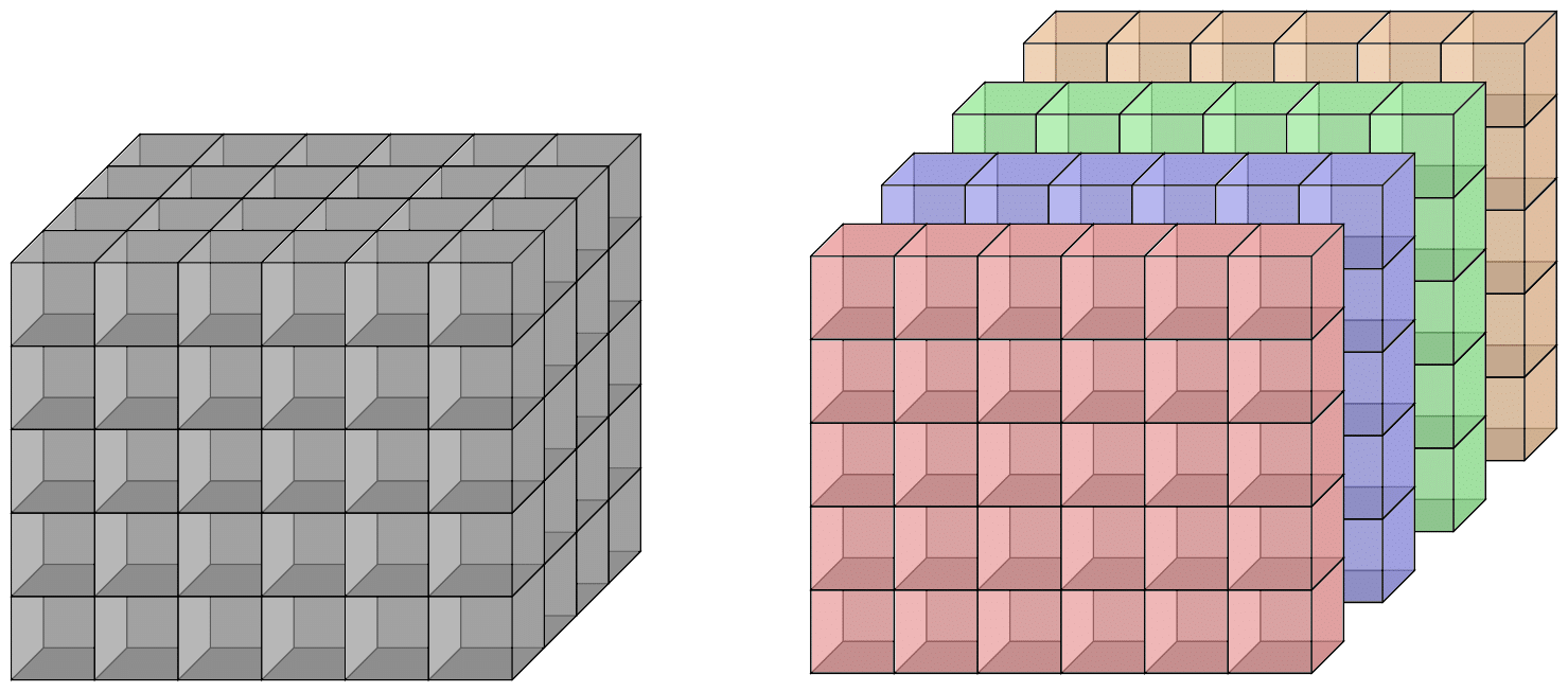

The equation $\langle t | Xu, v\rangle = Z\langle t | u, v\rangle$ becomes

XT^{*}_{*j} - T^{*}_{*j}Z = 0,

where $T^{*}_{*j}$ is the $j$ th slice in the $1$ -coordinate as a matrix:

T_{*j}^{*} = \begin{bmatrix} t_{1j}^{1} & t_{1j}^{2} & \cdots \\ t_{2j}^{1} & t_{2j}^{2} & \cdots \\ \vdots & \vdots & \ddots \end{bmatrix}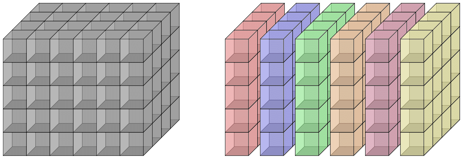

Solving simultaneous Sylvester systems: $\textsf{Sylver}$

These algorithms are part of a general family of Sylvester-like equations:

XA + BY = C.

We need to solve a simultaneous system of Sylvester-like equations.

Naively, this requires $O(d^7)$ field operations for a $(d\times d\times d)$ -grid.

In general, construct a basis of the kernel of a

$(d_0\cdots d_n) \times (d_0^2 +\cdots + d_n^2)$ -matrix.

Theorem (M.-Wilson 2018).

There is an algorithm to solve simultaneous Sylvester equations of a nondegenerate

(d\times d\times d)

-grid using

O(d^4)

field operations.

Open: Extend this to general tensors and implement.

Tensor spaces & tensor categories

Tensor spaces are the spaces containing tensors. Therefore, defined similarly to tensors.

A tensor space $T$ is a $K$ -vector space with

1. a frame $(U_0, \ldots, U_n)$ ,

2. an interpreter map $\langle \cdot | : T\rightarrow \left( U_n\times \cdots \times U_1\rightarrowtail U_0\right)$ ,

3. a category,

4. a basis.

The map $\langle \cdot |$ gives every $t\in T$ a multilinear map interpretation

$\langle t | : U_n\times \cdots \times U_1\rightarrowtail U_0.$

Examples that hint towards tensor categories

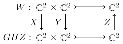
Equivalence up to a change of bases. The states $GHZ$ and $W$ are inequivalent.

For all $X, Y, Z\in \text{GL}_2(\mathbb{C})$ , there exists $u, v\in\mathbb{C}^2$ such that

$\begin{aligned} Z\langle GHZ | Xu, Yv\rangle \ne \langle W | u, v \rangle. \end{aligned}$

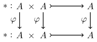
Equivalence of algebras: an isomorphism.

There exists $\varphi\in\text{GL}(A)$ such that for all $a,b\in A$

$\begin{aligned} \varphi(ab) &= \varphi(a)\varphi(b). \end{aligned}$

Adjoint operators of a bilinear form $\langle\,,\,\rangle$ .

For $u,v\in V$ , and $A\in \text{GL}(V)$ ,

\begin{aligned} \langle Au, v \rangle &= \langle u, A^*v\rangle. \end{aligned}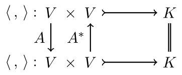

A data structure for tensor categories

For us a tensor category is

1. a function $\textsf{A}: [n] \rightarrow \{-1, 0, 1\}$ ,

2. a partition of $[n]$ .

The function $\textsf{A}$ tells us which way the arrows go: $\downarrow$ , $\parallel$ , or $\uparrow$ .

The partition tells us which coordinates are treated as equal.

Examples in $\textsf{TensorSpace}$

Let's look at a tensor created earlier: the multiplication in an algebra

$\langle t | : \text{M}_2(\mathbb{Q}) \times \text{M}_2(\mathbb{Q}) \rightarrowtail \text{M}_2(\mathbb{Q}).$

A := MatrixAlgebra(Q, 2);
t := Tensor(A);
TensorCategory(t);

Tensor category of valence 3 (->,->,->) ({ 0, 1, 2 })

all arrows are $\downarrow$ , and
an operator acts the same way in all three coordinates.

Let's look at an example as a high-dimensional grid.

t := Tensor(GF(2), [2, 3, 2, 3], [1..36]);
t;

Tensor of valence 4, U3 x U2 x U1 >-> U0
U3 : Full Vector space of degree 2 over GF(2)
U2 : Full Vector space of degree 3 over GF(2)
U1 : Full Vector space of degree 2 over GF(2)
U0 : Full Vector space of degree 3 over GF(2)

The default tensor category is given.

TensorCategory(t);          // default category

Tensor category of valence 4 (->,->,->,->) ({ 1 },{ 2 },{ 0 },{ 3 })

Relating tensor spaces & operators

Densor subspaces

The $GHZ$ and $W$ -state are not equivalent because derivations were not isomorphic.

For these kinds of questions, we consider spaces of all tensors sharing common operators.

Recall the derivation algebra of $t\in T$ ,

$\begin{aligned} \mathcal{D}_t &= \{ (X, Y, Z) \in \Omega \mid \forall u, v,\; \langle t | Xu, v\rangle + \langle t | u, Yv\rangle = Z\langle t | u, v\rangle\} \end{aligned}$

For $t\in T$ , the densor subsapce of $t$ is the tensor subspace

$\textsf{Dens}(t) = \{ s\in T \mid \mathcal{D}_t \subseteq \mathcal{D}_s \}.$

Example from Lie algebras

Lie algebra of $3\times 3$ trace zero matrices over a field $K$ , denoted $\mathfrak{sl}_3$ .

The tensor given by the matrix commutator is the following.

K := GF(7);
sl3 := LieAlgebra("A2", K);
t := Tensor(sl3);
t;

Tensor of valence 3, U2 x U1 >-> U0
U2 : Full Vector space of degree 8 over GF(7)
U1 : Full Vector space of degree 8 over GF(7)
U0 : Full Vector space of degree 8 over GF(7)

Few tensors contain an

8

-dimensional Lie algebra.

Note the tensor category.

TensorCategory(t);

Tensor category of valence 3 (->,->,->) ({ 0, 1, 2 })

Each operator acts the same on each of the three coordinates.

From standard results, $\mathcal{D}_t \cong \mathfrak{sl}_3$ .

D := DerivationAlgebra(t);
Dimension(D);

The densor subspace of $t$ is computed using $\textsf{Densor}$ .

Dens := UniversalDensorSubspace(t); 
Dens;

Tensor space of dimension 2 over GF(7) with valence 3
U2 : Full Vector space of degree 8 over GF(7)
U1 : Full Vector space of degree 8 over GF(7)
U0 : Full Vector space of degree 8 over GF(7)

The dimension of the densor subspace is tiny compared to the ambient space.

T := Parent(t);                      // full tensor space of t
Dimension(T), Dimension(Dens);

512 2

What just happened?

Example: matrix multiplication

The tensor space $T$ framed by $(K^{12}, K^8, K^6)$ contains

\langle t | : \text{M}_{3\times 4} \times \text{M}_{4\times 2} \rightarrowtail \text{M}_{3\times 2}.

t := MatrixTensor(Q, [3, 4, 2]);
t;

Tensor of valence 3, U2 x U1 >-> U0
U2 : Full Vector space of degree 12 over Rational Field
U1 : Full Vector space of degree 8 over Rational Field
U0 : Full Vector space of degree 6 over Rational Field

The derivation algebra of $t$ is large because matrix multiplication is distributive.

Recall the derivation equation:

$\langle t | Xu, v\rangle + \langle t | u, Yv \rangle = Z\langle t | u, v \rangle$

If $X\in \text{M}_{3\times 3}$ , then we re-interpret

$(XU)*V + U*(0V) = X(U*V).$

Similar equations hold for $Y\in\text{M}_{4\times 4}$ and $Z\in\text{M}_{2\times 2}$ .

Therefore, $\text{M}_{3\times 3} \cup \text{M}_{4\times 4} \cup \text{M}_{2\times 2} \subseteq \mathcal{D}_t$ .

We denote the algebra $\text{M}_{n\times n}$ with the matrix commutator by $\mathfrak{gl}_n$ .

Fact. $\mathcal{D}_t \cong \left(\mathfrak{gl}_3\oplus \mathfrak{gl}_4 \oplus\mathfrak{gl}_2\right)/K$ .

D := DerivationAlgebra(t);
Dimension(D) eq (3^2 + 4^2 + 2^2 - 1);           // compare dimensions

We can easily verify that the dimensions match.

true

Dens := UniversalDensorSubspace(t);
Dens;

Tensor space of dimension 1 over Rational Field with valence 3
U2 : Full Vector space of degree 12 over Rational Field
U1 : Full Vector space of degree 8 over Rational Field
U0 : Full Vector space of degree 6 over Rational Field

With derivaton algebra so large, the densor subspace must be small.

Therefore, in a $576$ -dimensional space, $T$ , matrix multiplication is set apart from the rest.

As a consequence, the symmetries of $t$ are completely determined by its derivations.

How are densor spaces computed?

A dual solve to derivations

Recall, we consider Sylvester-like systems of the form:

$XT_{**}^{(k)} + T_{**}^{(k)}Y = 0$

The same system is used to get the densor subspace$-$the roles are swapped.

We are given the derivation algebra, so we slice a symbolic tensor.

Simultaneously solve a "dual" version of the Sylvester-like equations.

Theorem. (Brooksbank-M.-Wilson)

There exists an algorithm to simultaneously solve a "dual" Sylvester-like system using $O(d^9m^2)$ field operations, given $m$ operators acting on a $(d\times d\times d)$ -grid.

Open: Does a similar improvement apply for these equations as well? What is the resulting complexity?

Summary

Still uncovering new algebraic data from tensors, and this is a snapshot of $\textsf{TensorSpace}$ .

Context through the frame and tensor category give flexibility in the data structures.

These algebras provide general tools to different kinds of applications.