Exponential Box-splines

For use in Visualization

Joshua Horacsek

Motivation

  • Regularly sampled data                                                      
  • Continous
  • Differentiable
  • Compact  

Refresher: B-splines

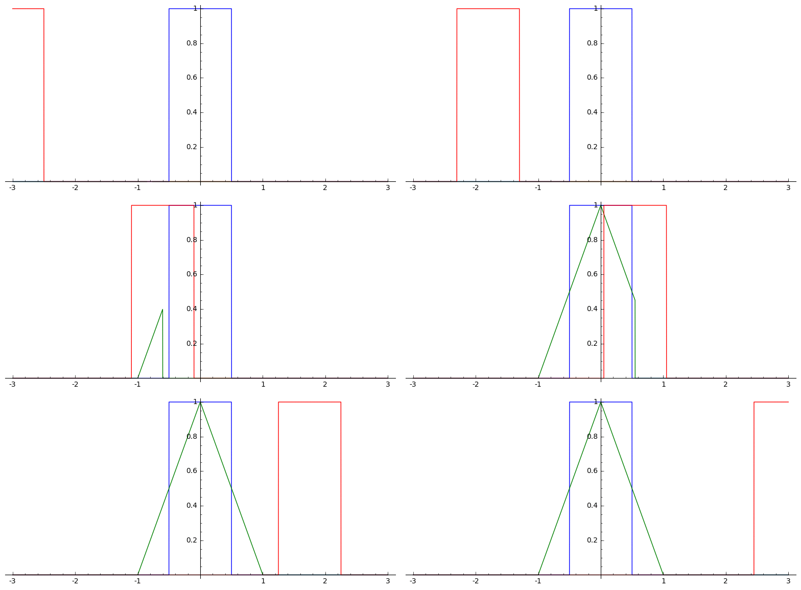
B-splines can be defined as successive convolutions of the box function with itself

\beta_0(x) = \begin{cases} 1 & -1/2 < x < 1/2 \\ 0 & \text{otherwise} \end{cases}
β0(x)={11/2<x<1/20otherwise\beta_0(x) = \begin{cases} 1 & -1/2 < x < 1/2 \\ 0 & \text{otherwise} \end{cases}

Refresher: B-splines

B-splines can be defined as successive convolutions of the box function with itself

(f * g)(x) = \int_{-\infty}^{\infty}f(x)g(x-\tau)d\tau
(fg)(x)=f(x)g(xτ)dτ(f * g)(x) = \int_{-\infty}^{\infty}f(x)g(x-\tau)d\tau
\beta_1(x) = (\beta_0 * \beta_0)(x)
β1(x)=(β0β0)(x)\beta_1(x) = (\beta_0 * \beta_0)(x)
\beta_2(x) = (\beta_0 * \beta_0 * \beta_0)(x)
β2(x)=(β0β0β0)(x)\beta_2(x) = (\beta_0 * \beta_0 * \beta_0)(x)
\beta_n(x) = (\beta_0 * \cdots * \beta_0)(x)
βn(x)=(β0β0)(x)\beta_n(x) = (\beta_0 * \cdots * \beta_0)(x)
n+1 \text{ times}
n+1 timesn+1 \text{ times}

Example: Linear B-spline

\beta_1(x) = (\beta_0 * \beta_0)(x)
β1(x)=(β0β0)(x)\beta_1(x) = (\beta_0 * \beta_0)(x)

Example: Quadratic B-spline

\beta_2(x) = ((\beta_0 * \beta_0) * \beta_0)(x)
β2(x)=((β0β0)β0)(x)\beta_2(x) = ((\beta_0 * \beta_0) * \beta_0)(x)
\beta_2(x) = (\beta_1 * \beta_0)(x)
β2(x)=(β1β0)(x)\beta_2(x) = (\beta_1 * \beta_0)(x)

Approximation

This is one big reason we care about B-splines

Start with a function

Approximation

Sample it

Approximation

f_i
fif_i

We now have samples

Approximation

\tilde{f}(x) = \sum f_i\beta_1(x-i)
f~(x)=fiβ1(xi)\tilde{f}(x) = \sum f_i\beta_1(x-i)

Reconstruct function with basis functions

Approximation

\tilde{f}(x) = \sum f_i\beta_1(x-i)
f~(x)=fiβ1(xi)\tilde{f}(x) = \sum f_i\beta_1(x-i)

Reconstruct function with basis functions

Approximation

\tilde{f}(x) = \sum f_i\beta_1(x-i)
f~(x)=fiβ1(xi)\tilde{f}(x) = \sum f_i\beta_1(x-i)

Reconstruct function with basis functions

Approximation

\tilde{f}(x) = \sum f_i\beta_2(x-i)
f~(x)=fiβ2(xi)\tilde{f}(x) = \sum f_i\beta_2(x-i)

Potential pitfall

Approximation

\tilde{f}(x) = \sum f_i\beta_2(x-i)
f~(x)=fiβ2(xi)\tilde{f}(x) = \sum f_i\beta_2(x-i)

Potential pitfall

Approximation

\tilde{f}(x) = \sum f_i\beta_2(x-i)
f~(x)=fiβ2(xi)\tilde{f}(x) = \sum f_i\beta_2(x-i)

Potential pitfall

Approximation

\tilde{f}(x) = \sum c_i\beta_2(x-i)
f~(x)=ciβ2(xi)\tilde{f}(x) = \sum c_i\beta_2(x-i)

Quasi-interpolation

c_i := -\frac{1}{2}f_{i-1} + 2f_i - \frac{1}{2}f_{i+1}
ci:=12fi1+2fi12fi+1c_i := -\frac{1}{2}f_{i-1} + 2f_i - \frac{1}{2}f_{i+1}

Exponential B-splines

Exponential B-splines can be defined as successive convolutions of an exponentially weighted box function with another

\beta_{(\alpha)}(x) = \begin{cases} e^{\alpha(x+1/2)} & -1/2 < x < 1/2 \\ 0 & \text{otherwise} \end{cases}
β(α)(x)={eα(x+1/2)1/2<x<1/20otherwise\beta_{(\alpha)}(x) = \begin{cases} e^{\alpha(x+1/2)} & -1/2 < x < 1/2 \\ 0 & \text{otherwise} \end{cases}

Exponential B-splines

Exponential B-splines can be defined as successive convolutions of an exponentially weighted box function with another

(f * g)(x) = \int_{-\infty}^{\infty}f(x)g(x-\tau)d\tau
(fg)(x)=f(x)g(xτ)dτ(f * g)(x) = \int_{-\infty}^{\infty}f(x)g(x-\tau)d\tau
\beta_{(\alpha_1, \alpha_2)}(x) = (\beta_{(\alpha_0)} * \beta_{(\alpha_1)} )(x)
β(α1,α2)(x)=(β(α0)β(α1))(x)\beta_{(\alpha_1, \alpha_2)}(x) = (\beta_{(\alpha_0)} * \beta_{(\alpha_1)} )(x)
\beta_{(\alpha_1, \alpha_2, \alpha_3)}(x) = (\beta_{(\alpha_0)} * \beta_{(\alpha_1)} * \beta_{(\alpha_2)} )(x)
β(α1,α2,α3)(x)=(β(α0)β(α1)β(α2))(x)\beta_{(\alpha_1, \alpha_2, \alpha_3)}(x) = (\beta_{(\alpha_0)} * \beta_{(\alpha_1)} * \beta_{(\alpha_2)} )(x)
\vdots
\vdots

Example: Exponential B-spline

\beta_{(\frac{1}{2}, -\frac{1}{2})}(x) = (\beta_{(\frac{1}{2})} * \beta_{(-\frac{1}{2})} )(x)
β(12,12)(x)=(β(12)β(12))(x)\beta_{(\frac{1}{2}, -\frac{1}{2})}(x) = (\beta_{(\frac{1}{2})} * \beta_{(-\frac{1}{2})} )(x)

Example: Exponential B-spline

\beta_{(\frac{1}{2}, 0)}(x) = (\beta_{(\frac{1}{2})} * \beta_{(0)} )(x)
β(12,0)(x)=(β(12)β(0))(x)\beta_{(\frac{1}{2}, 0)}(x) = (\beta_{(\frac{1}{2})} * \beta_{(0)} )(x)

Properties

  • Locally an exponential polynomial
  • Infinitely differentiable everywhere except knot points
  • Stable basis (Riesz basis)
  • Partition of unity/approximation order?

Last point not so clear -- need to look at 

\alpha_i
αi\alpha_i

Box-splines

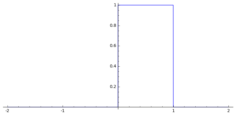
Box-splines are piecewise polynomial functions a can be obtained from successive convolutions of the box function in specific directions

X := \begin{bmatrix} | & | & \ & | \\ \xi_1 & \xi_2 & \cdots & \xi_n \\ | & | & \ & | \end{bmatrix}
X:=[ ξ1ξ2ξn ]X := \begin{bmatrix} | & | & \ & | \\ \xi_1 & \xi_2 & \cdots & \xi_n \\ | & | & \ & | \end{bmatrix}

Box-splines

Box-splines are piecewise polynomial functions a can be obtained from successive convolutions of the box function in specific directions
Box-splines
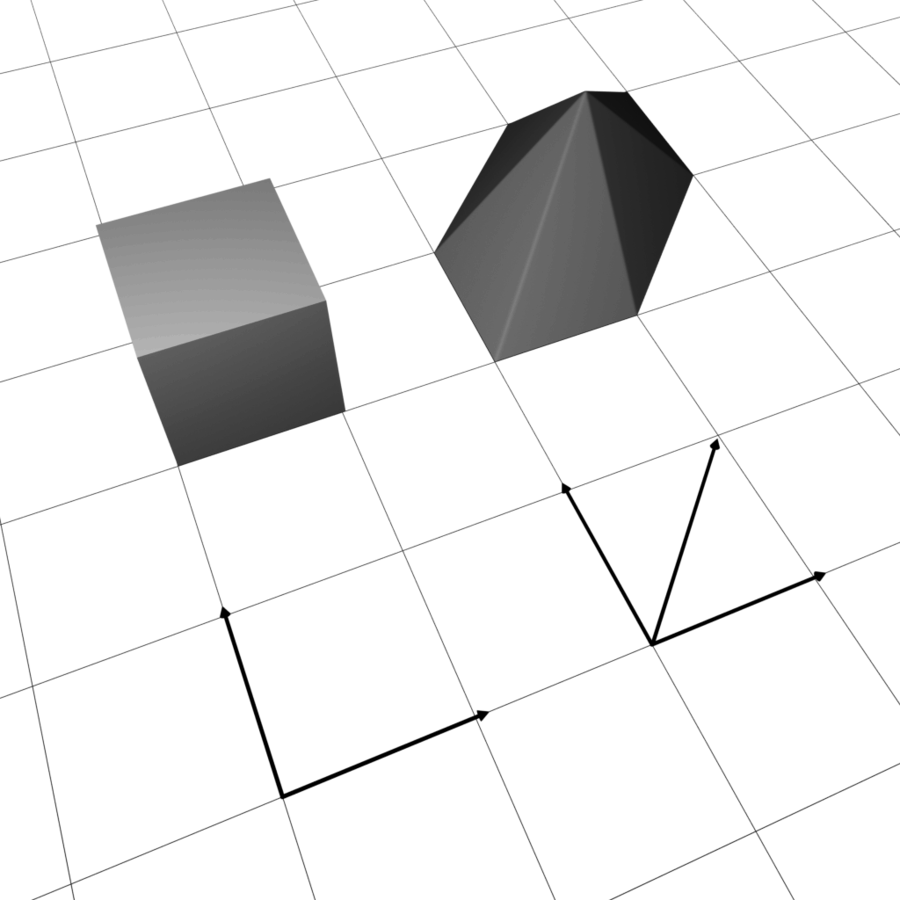
Example: Courant Element
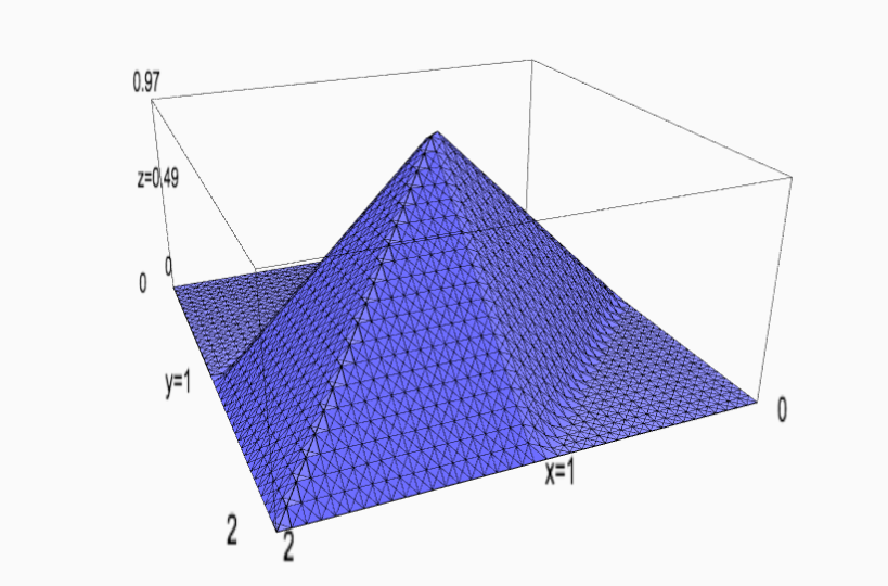
X := \begin{bmatrix} 1 & 0 & 1 \\ 0 & 1 & 1 \end{bmatrix}
X:=[101011]X := \begin{bmatrix} 1 & 0 & 1 \\ 0 & 1 & 1 \end{bmatrix}

Approximation

Approximation

Approximation
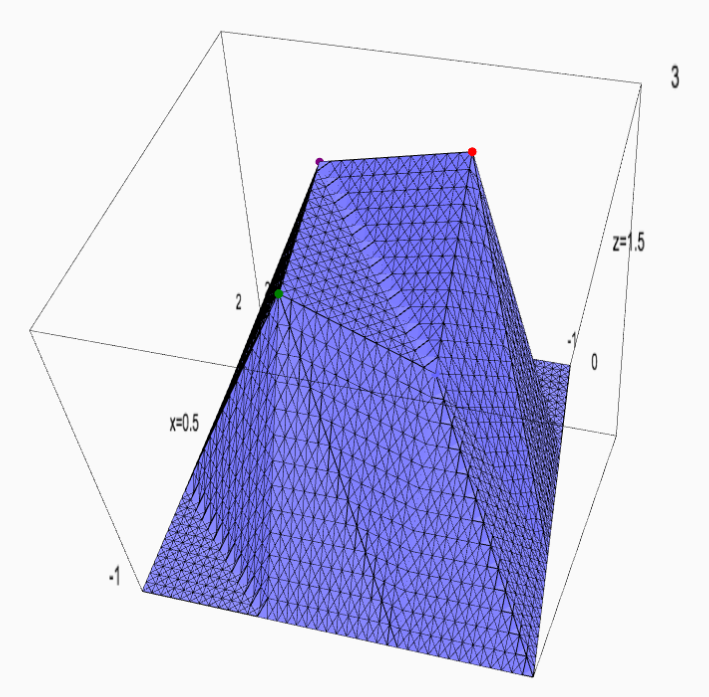
Exponential Box-splines

Exponential Box-splines can be obtained from successive convolutions of the exponentially weighted box function in specific directions

X := \begin{bmatrix} | & | & \ & | \\ \xi_1 & \xi_2 & \cdots & \xi_n \\ | & | & \ & | \end{bmatrix}
X:=[ ξ1ξ2ξn ]X := \begin{bmatrix} | & | & \ & | \\ \xi_1 & \xi_2 & \cdots & \xi_n \\ | & | & \ & | \end{bmatrix}
\Gamma := \begin{bmatrix} \gamma_1 & \gamma_2 & \cdots & \gamma_n \end{bmatrix}
Γ:=[γ1γ2γn]\Gamma := \begin{bmatrix} \gamma_1 & \gamma_2 & \cdots & \gamma_n \end{bmatrix}

Exponential Box-splines

X := \begin{bmatrix} 1 & 0 \\ 0 & 1 \end{bmatrix}
X:=[1001]X := \begin{bmatrix} 1 & 0 \\ 0 & 1 \end{bmatrix}
\Gamma := \begin{bmatrix} \frac{1}{2} & 0 \end{bmatrix}
Γ:=[120]\Gamma := \begin{bmatrix} \frac{1}{2} & 0 \end{bmatrix}
X := \begin{bmatrix} 1 & 0 & 1\\ 0 & 1 & 1 \end{bmatrix}
X:=[101011]X := \begin{bmatrix} 1 & 0 & 1\\ 0 & 1 & 1 \end{bmatrix}
\Gamma := \begin{bmatrix} \frac{1}{2} & 0 & 0 \end{bmatrix}
Γ:=[1200]\Gamma := \begin{bmatrix} \frac{1}{2} & 0 & 0 \end{bmatrix}

Exponential Box-splines

X := \begin{bmatrix} 1 & 0 & 1\\ 0 & 1 & 1 \end{bmatrix}
X:=[101011]X := \begin{bmatrix} 1 & 0 & 1\\ 0 & 1 & 1 \end{bmatrix}
\Gamma := \begin{bmatrix} \frac{1}{2} & 0 & 0 \end{bmatrix}
Γ:=[1200]\Gamma := \begin{bmatrix} \frac{1}{2} & 0 & 0 \end{bmatrix}

Exponential Box-splines

X := \begin{bmatrix} 1 & 0 & 1\\ 0 & 1 & 1 \end{bmatrix}
X:=[101011]X := \begin{bmatrix} 1 & 0 & 1\\ 0 & 1 & 1 \end{bmatrix}
\Gamma := \begin{bmatrix} a & 0 & 0 \end{bmatrix}
Γ:=[a00]\Gamma := \begin{bmatrix} a & 0 & 0 \end{bmatrix}
a \in \{-2, -1, -1/2, 1/2\}
a{2,1,1/2,1/2}a \in \{-2, -1, -1/2, 1/2\}

Properties

  • Locally an exponential polynomial
  • Infinitely differentiable everywhere except knot planes
  • Stable basis (Riesz basis, sometimes...)
  • Partition of unity/approximation order?

Last point not so clear -- need to look at 

\Gamma
Γ\Gamma

Questions

  • Fidelity?  
  • Symmetry?
  • Approximation order?                                                                            

Again, need to look at 

\Gamma
Γ\Gamma

Thanks!

Questions?