Bridging Simulators with Conditional Optimal Transport
Justine Zeghal, Benjamin Remy,
Yashar Hezaveh, François Lanusse,
Laurence Perreault-Levasseur


Advancing Field-level and Simulation-based Inference for Cosmology
Perimeter Institute for Theoretical Physics, Canada
June 2026
Cosmological Inference
Cosmological Inference
Cosmological Inference
Bayes theorem:
Cosmological Inference
Bayes theorem:
Cosmological Inference
Bayes theorem:

Cosmological Inference
Bayes theorem:
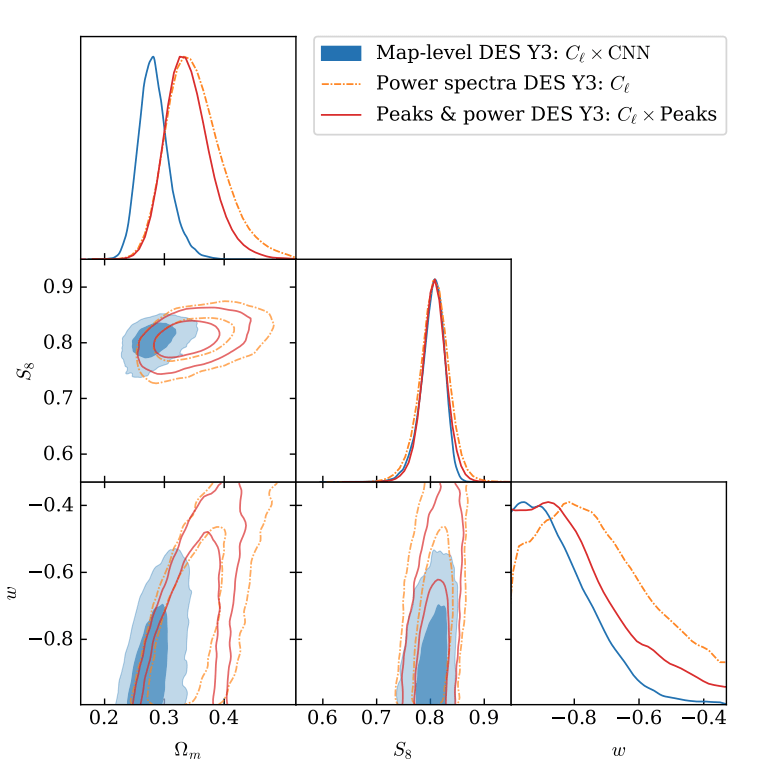
DES Y3 Results (with SBI).

Stage III
Stage IV
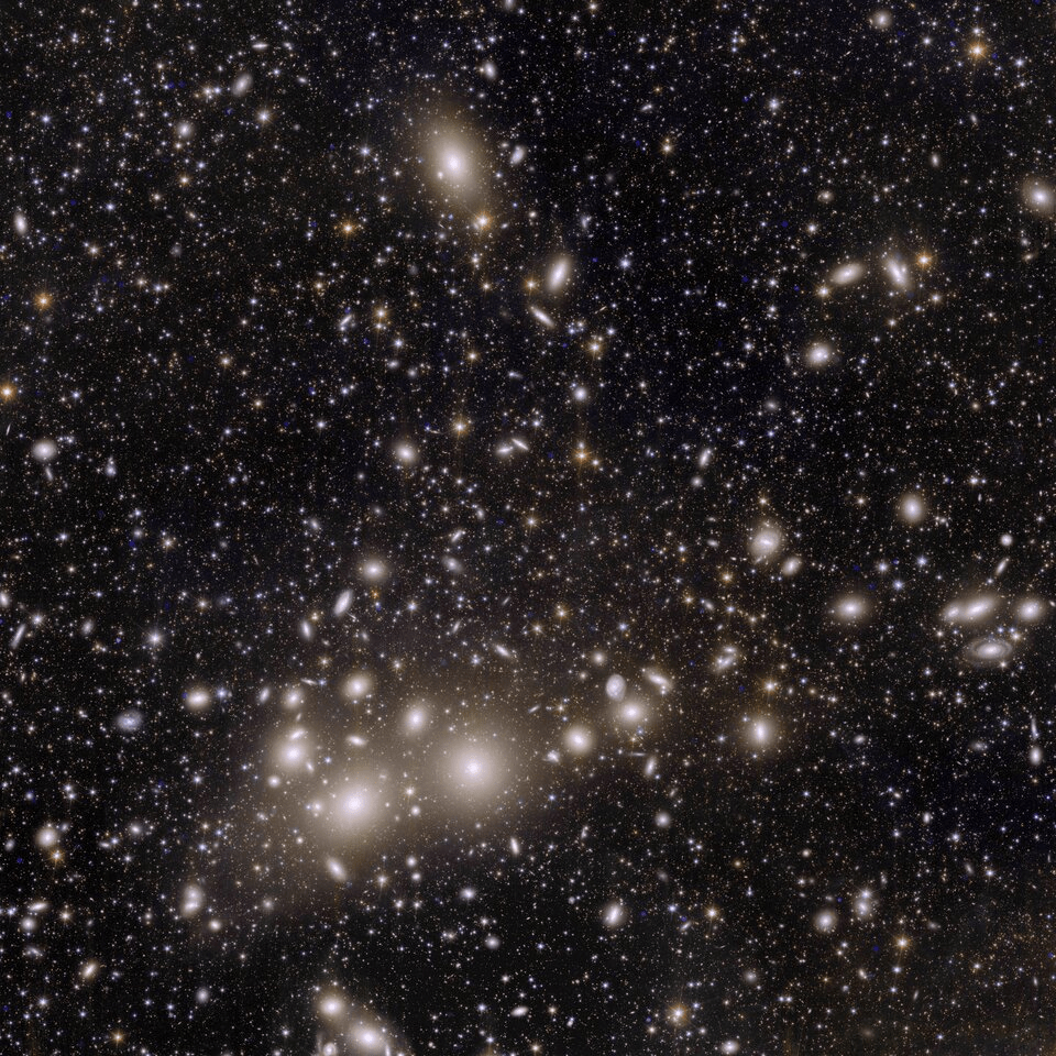
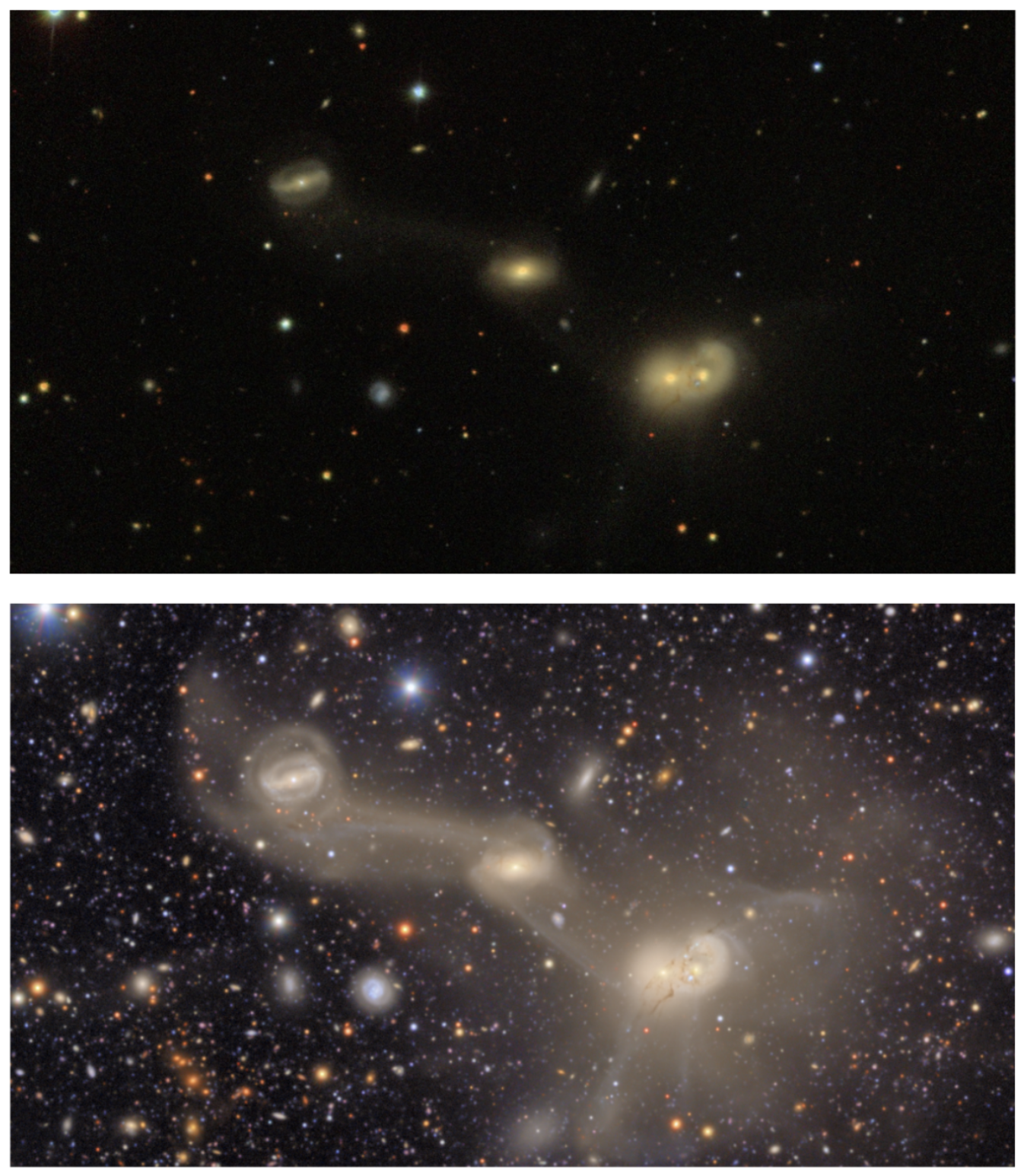
Portion of the Virgo cluster, zoom on RSCG 55
Portion of the Virgo cluster, zoom on RSCG 55
Cosmological Surveys
Full-field inference: extracting all cosmological information
Full-field inference: extracting all cosmological information
Bayes theorem:
Full-field inference: extracting all cosmological information
Simulator
Bayes theorem:
Full-field inference: extracting all cosmological information
Simulator
Two ways to get the posterior:
- Explicit inference:
- Implicit inference:
Bayes theorem:
Full-field inference: extracting all cosmological information
Simulator
Two ways to get the posterior:
- Explicit inference:
- Implicit inference:
Has to be realistic!
Bayes theorem:
Wrong models generate bias
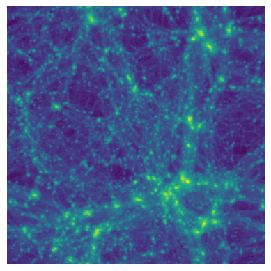
Fast simulations
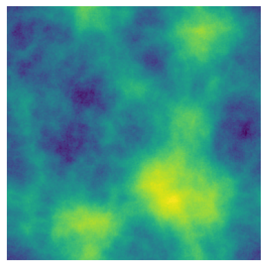
Costly simulations
Wrong models generate bias
→ e.g. full nbody, hydro
Fast simulations
Costly simulations
| O(ms) runtime | ❌ |
| differentiable | ❌ |
| realistic | ✅ |
Wrong models generate bias
→ e.g. full nbody, hydro
→ e.g. log-normal, LPT, PM
| O(ms) runtime | ✅ |
| differentiable | ✅ |
| realistic | ❌ |
Fast simulations
Costly simulations
| O(ms) runtime | ❌ |
| differentiable | ❌ |
| realistic | ✅ |
Learning the correction
We can learn
the correction!
Fast simulations
Costly simulations
Learning the correction
We can learn
the correction!
Fast simulations
- it preserves the conditioning,
Costly simulations
- ,
such that
- it minimally correct the simulation.
Learning the correction
We can learn
the correction!
Fast simulations
- it preserves the conditioning,
Costly simulations
- ,
such that
- it minimally correct the simulation.
Requirements:
- has to map to a distribution sample.
- has to work in high dimensions.
- has to bridge any two distributions.
- has to bridge conditional distributions.
- has to be the solution of the OT problem.
Conditional Optimal Transport Flow Matching
Conditional Optimal Transport Flow Matching
(Lipman et al. 2023)
Flow matching
(Lipman et al. 2023)
Flow matching
(Lipman et al. 2023)
Flow matching

Credit: Michael S. Albergo et al. 2023
(Lipman et al. 2023)
Flow matching
Credit: Michael S. Albergo et al. 2023
Credit: Gagneux et al. 2025
(Lipman et al. 2023)
Flow matching
with:
Credit: Michael S. Albergo et al. 2023
Credit: Tong et al. 2023
Credit: Gagneux et al. 2025
Requirements:
- has to map to a distribution sample.
- has to work in high dimensions.
- has to bridge any two distributions.
- has to bridge conditional distributions.
- has to be the solution of the OT problem.
✅
✅
✅
Conditional Optimal Transport Flow Matching
Requirements:
- has to map to a distribution sample.
- has to work in high dimensions.
- has to bridge any two distributions.
- has to bridge conditional distributions.
- has to be the solution of the OT problem.
✅
✅
✅
Conditional Optimal Transport Flow Matching
Optimal Transport
Definition:
OT seeks to find a minimal-effort mapping between distributions according to a cost C:
Optimal Transport
OT seeks to find a minimal-effort mapping between distributions according to a cost C:
Definition:
Optimal Transport
Definition:
OT seeks to find a minimal-effort mapping between distributions according to a cost C:
Optimal Transport
Definition:
OT seeks to find a minimal-effort mapping between distributions according to a cost C:
Optimal Transport
Definition:
OT seeks to find a minimal-effort mapping between distributions according to a cost C:
Optimal Transport
Definition:
OT seeks to find a minimal-effort mapping between distributions according to a cost C:
Flow Matching loss function:
Optimal Transport Flow Matching
(Tong et al. 2023)
Flow Matching loss function:
Indepent coupling:
Optimal Transport coupling:


Optimal Transport Flow Matching
(Tong et al. 2023)
Credit: Tong et al. 2023
Flow Matching loss function:
Indepent coupling:
Optimal Transport coupling:
i.e. minimizes the path for all trajectories between and .
This coupling, combined with the linear interpolant, solve the dynamic OT:
Optimal Transport Flow Matching
(Tong et al. 2023)
Credit: Tong et al. 2023
Requirements:
- has to map to a distribution sample.
- has to work in high dimensions.
- has to bridge any two distributions.
- has to bridge conditional distributions.
- has to be the solution of the OT problem.
✅
✅
✅
Conditional Optimal Transport Flow Matching
✅
Requirements:
- has to map to a distribution sample.
- has to work in high dimensions.
- has to bridge any two distributions.
- has to bridge conditional distributions.
- has to be the solution of the OT problem.
✅
✅
✅
Conditional Optimal Transport Flow Matching
✅
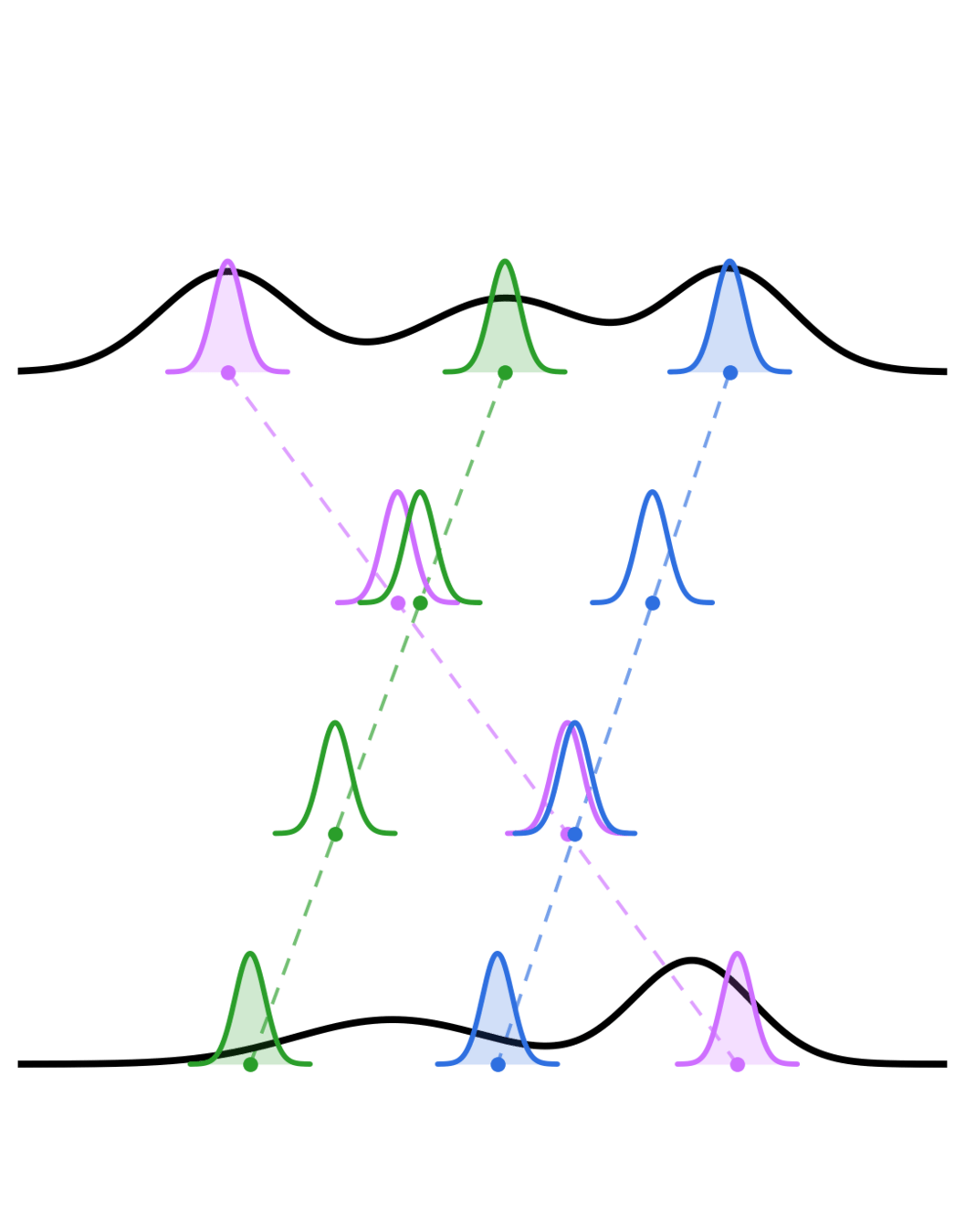
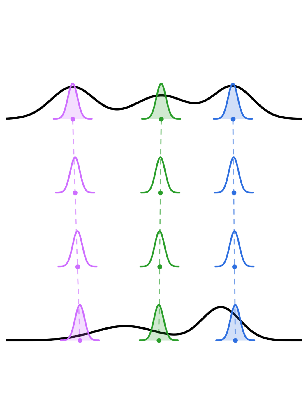
Conditional Optimal Transport Flow matching (Kerrigan et al. 2024)
OT Flow Matching loss function:
Dataset 1
Optimal Transport Plan
Dataset 2
Requirements:
- has to map to a distribution sample.
- has to work in high dimensions.
- has to bridge any two distributions.
- has to bridge conditional distributions.
- has to be the solution of the OT problem.
✅
✅
✅
✅
✅
→ e.g. full nbody, hydro
→ e.g. log-normal, LPT, PM
Fast simulations
Emulated simulations
| O(ms) runtime | ✅ |
| differentiable | ✅ |
| realistic | ❌ |
| O(ms) runtime | ✅ |
| differentiable | ✅ |
| relistic | ✅ |
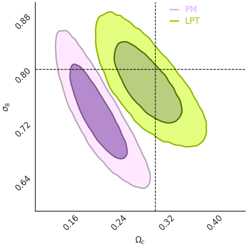
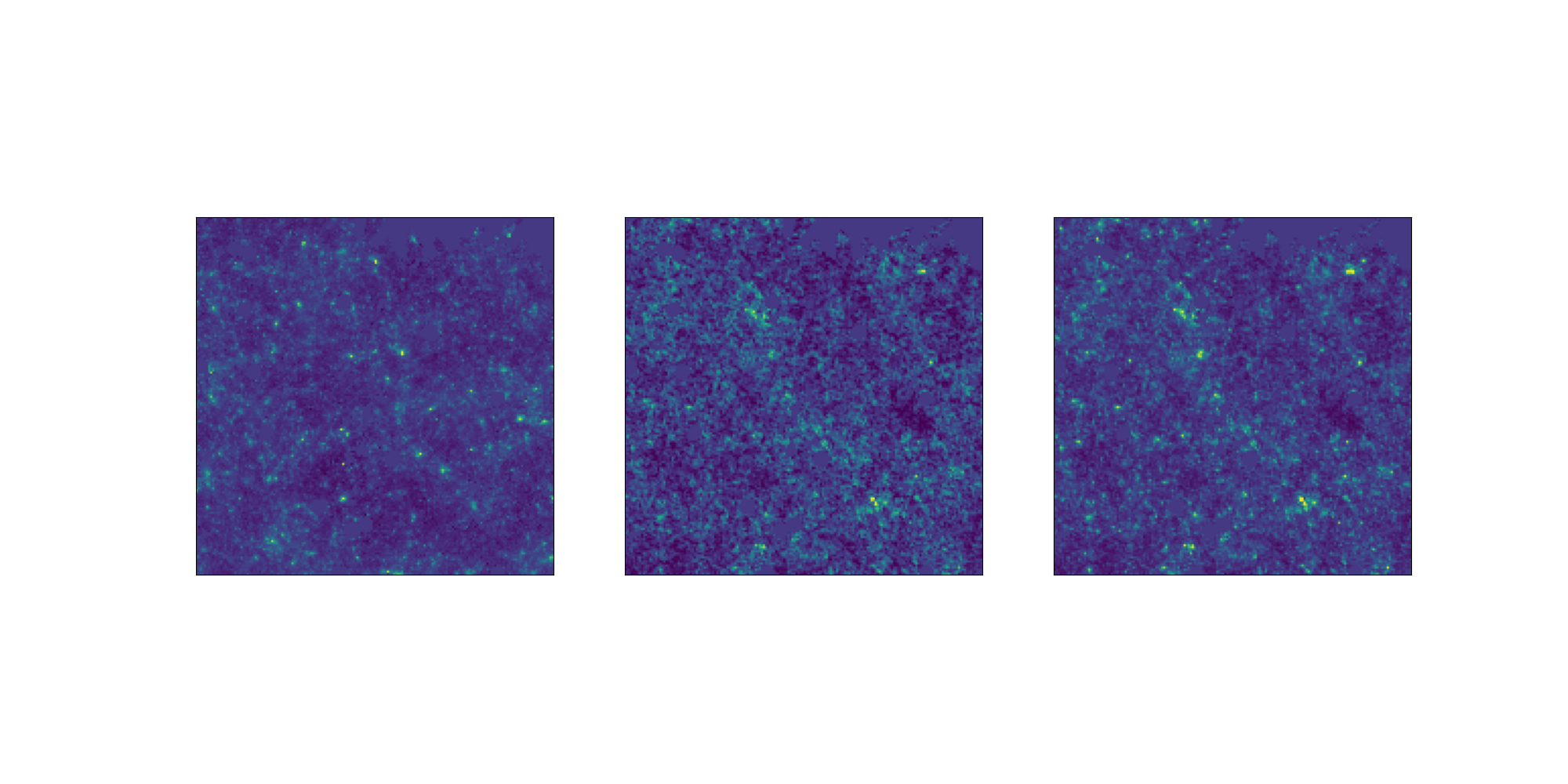
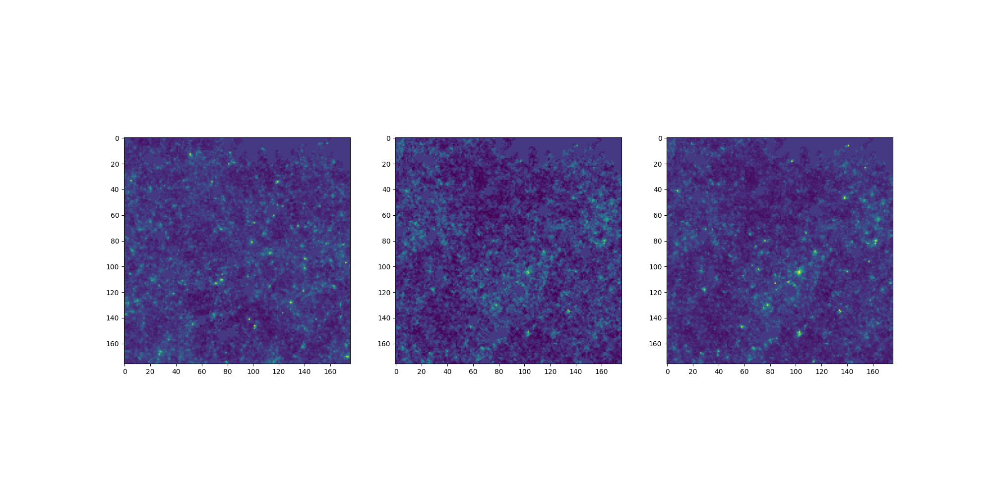
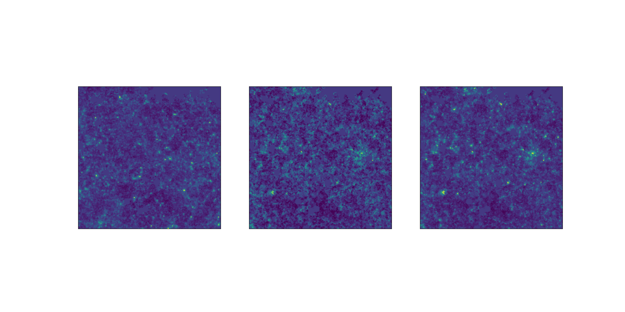
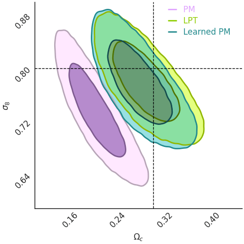
Results on weak lensing maps
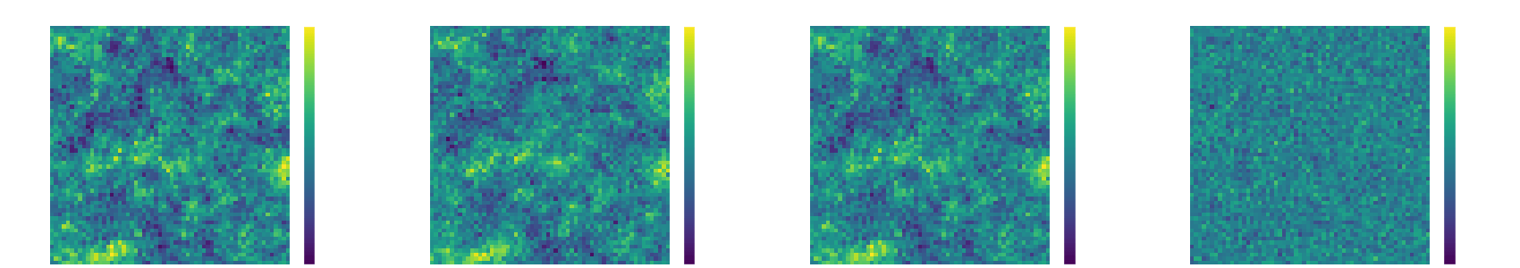
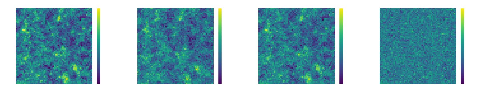
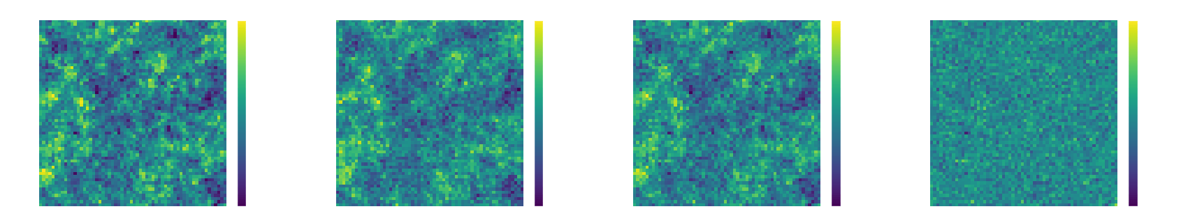
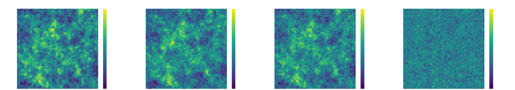
LPT
PM
Learned
Residuals
NeurIPS Challenge: Weak Lensing Uncertainty


CEA
France
Mila
Canada
UChicago
USA
CEA
France
NYU
USA
CEA
France
Mila
Canada
Univ. de Crète
Grèce
APC
France
Mila
Canada

Challenge simulation
NeurIPS Challenge: Weak Lensing Uncertainty
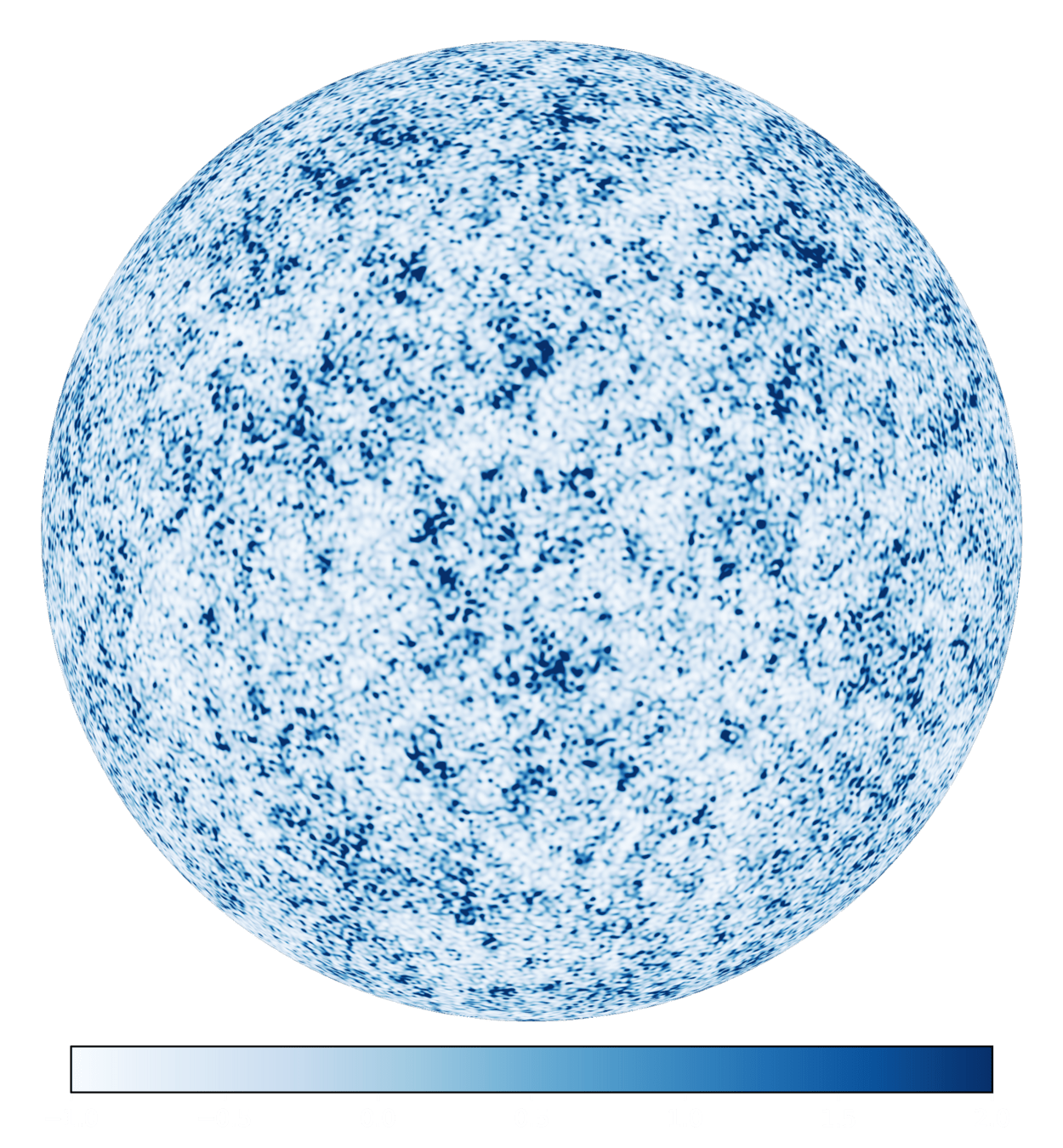
LogNormal Convergence (patch)


NeurIPS Challenge: Weak Lensing Uncertainty
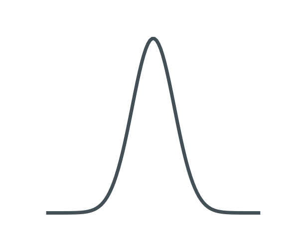
LogNormal
Challenge simulation
VS
NeurIPS Challenge: Weak Lensing Uncertainty
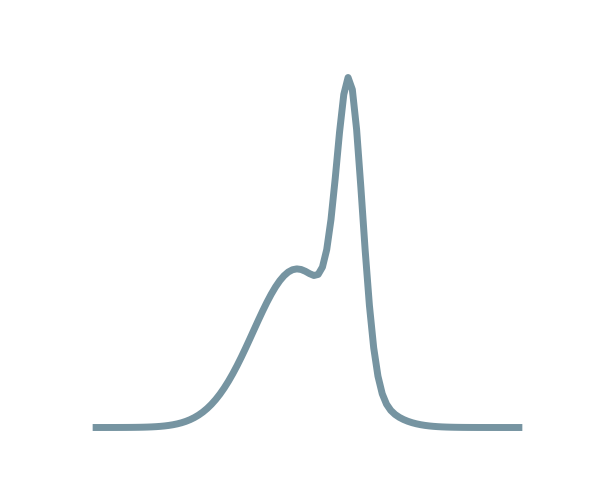
LogNormal
Challenge simulation
VS

Emulated
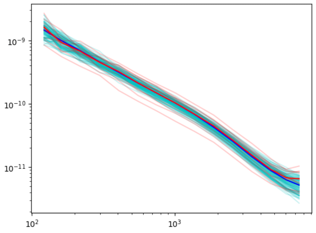
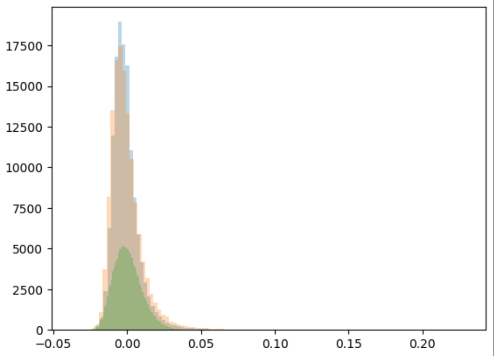
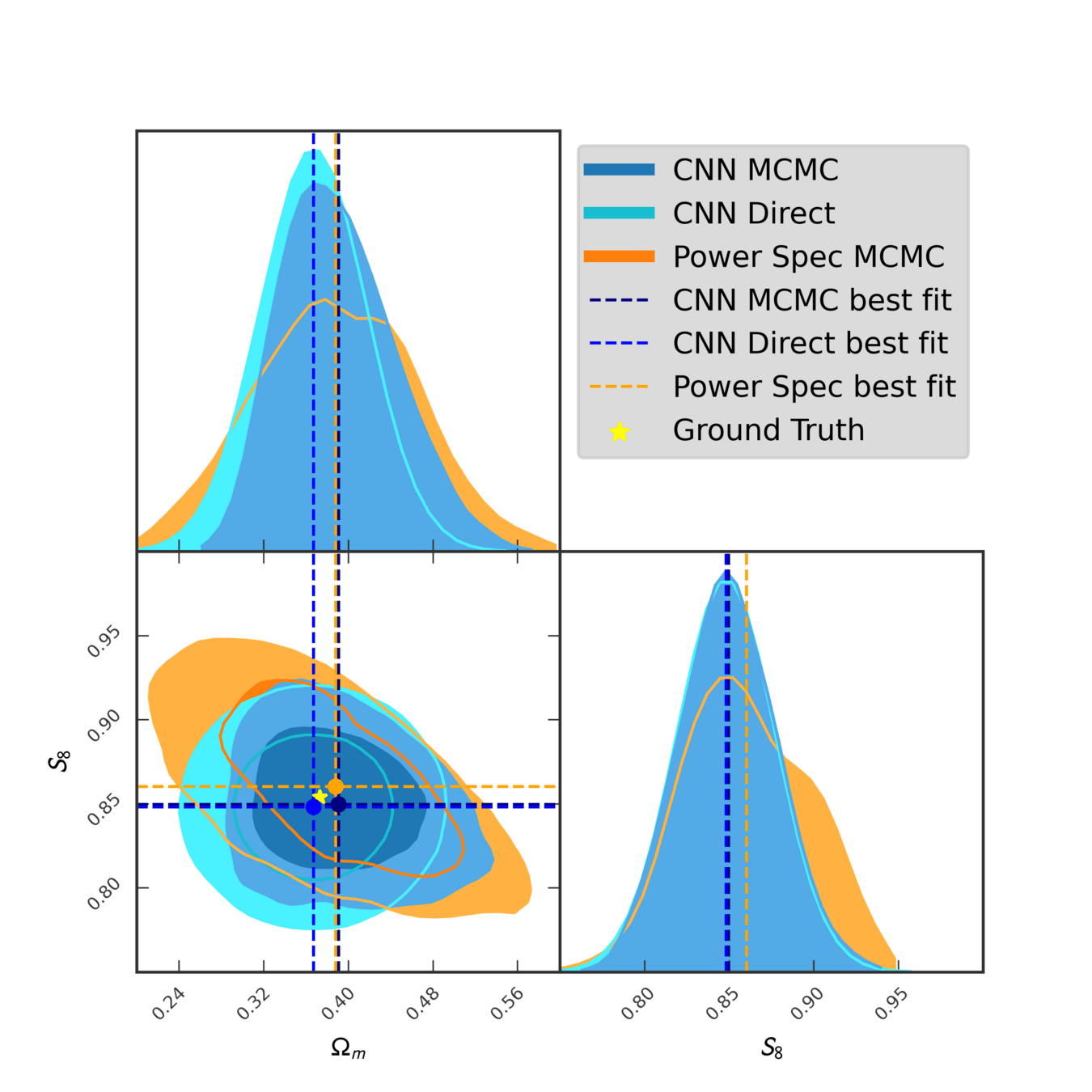
Power spectrum
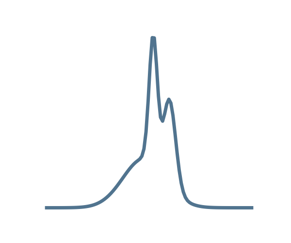
LogNormal
Emulated
Challenge simulation
VS
NeurIPS Challenge: Weak Lensing Uncertainty
LogNormal
Emulated
Challenge
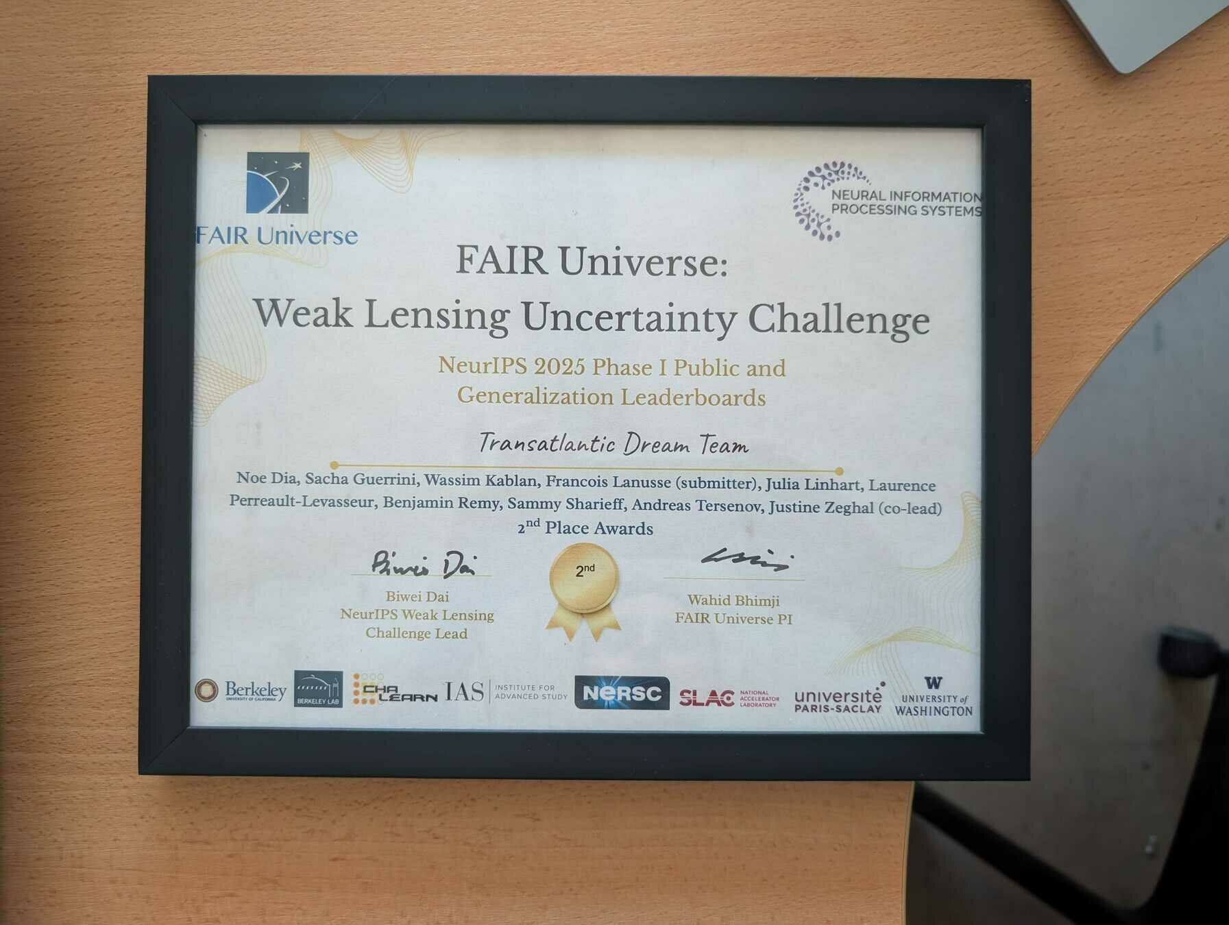
🥳
LogNormal
Emulated
Challenge simulation
VS
NeurIPS Challenge: Weak Lensing Uncertainty