Neural Compression and Neural Density Estimation for Cosmological Inference
PhD Defense, at APC, Paris
September 30, 2024
Justine Zeghal


Lambda Cold Dark Matter ( CDM)
The simplest model that best describes our observations is
Relying only on a few parameters:
Suggesting: ordinary matter, cold dark matter (CDM), and dark energy Λ as an explanation of the accelerated expansion.
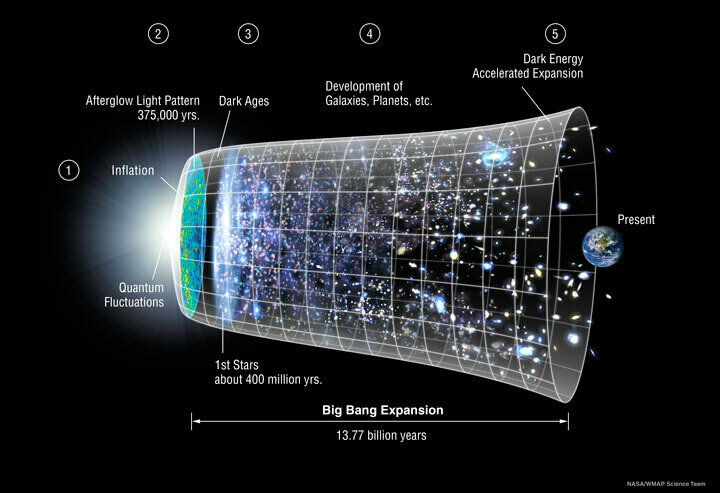
Goal: determine the value of those parameters based on our observations.
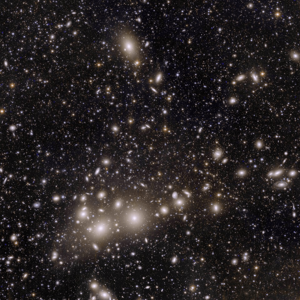
Credit: ESA
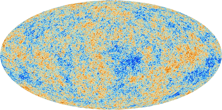
Credit: ESA and the Planck Collaboration
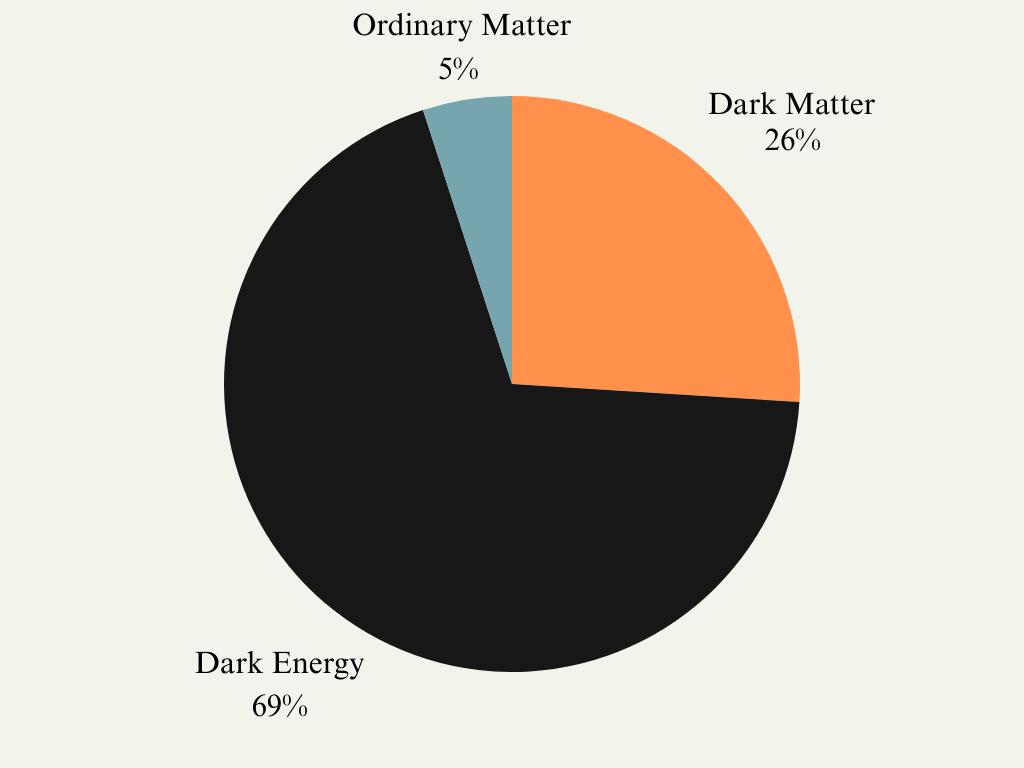
Mysterious components
Our universe is composed of 95% unknown components.
"Dark" because they do not interact electromagnetically.
→ Difficult to study their nature.
For instance, a question we would like to answer is whether dark energy is a cosmological constant or evolves with time?
we free the dark energy equation-of-state parameter
Dark Energy
We can study the impacts of
dark energy on large-scale structures of the Universe at different cosmic times.
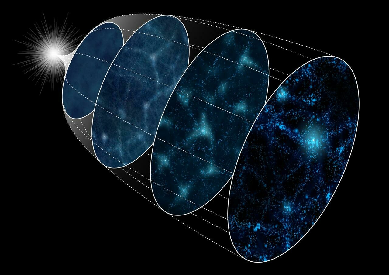
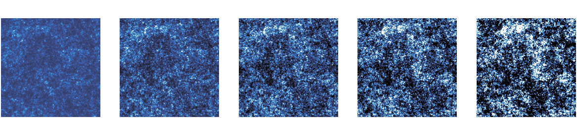
To study large-scale structures we need to map the distribution of matter in the Universe over time.
How to study something we cannot see?
Dark energy acts as a negative pressure that counteracts gravitational forces on large scales.
Gravitational Lensing
Credit: NASA's Goddard Space Flight Center Conceptual Image Lab
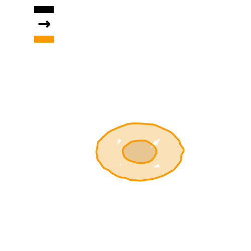
Weak Gravitational Lensing
Weak Gravitational Lensing
Galaxy shape
Weak Gravitational Lensing
Galaxy shape
Weak Gravitational Lensing
Galaxy shape
Convergence
Weak Gravitational Lensing
Galaxy shape
Convergence
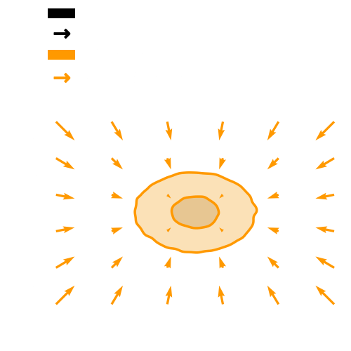
Shear
Weak Gravitational Lensing
Galaxy shape
Convergence
Shear
This phenomenon happens everywhere.
Weak Gravitational Lensing
Galaxy shape
Shear
This phenomenon happens everywhere.
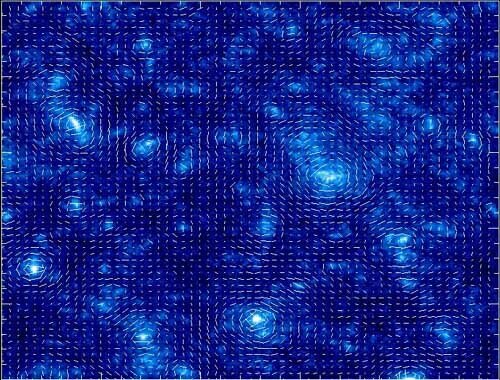
Credit: Alexandre Refregier and numerical simulations by Jain, Seljak & White 2000
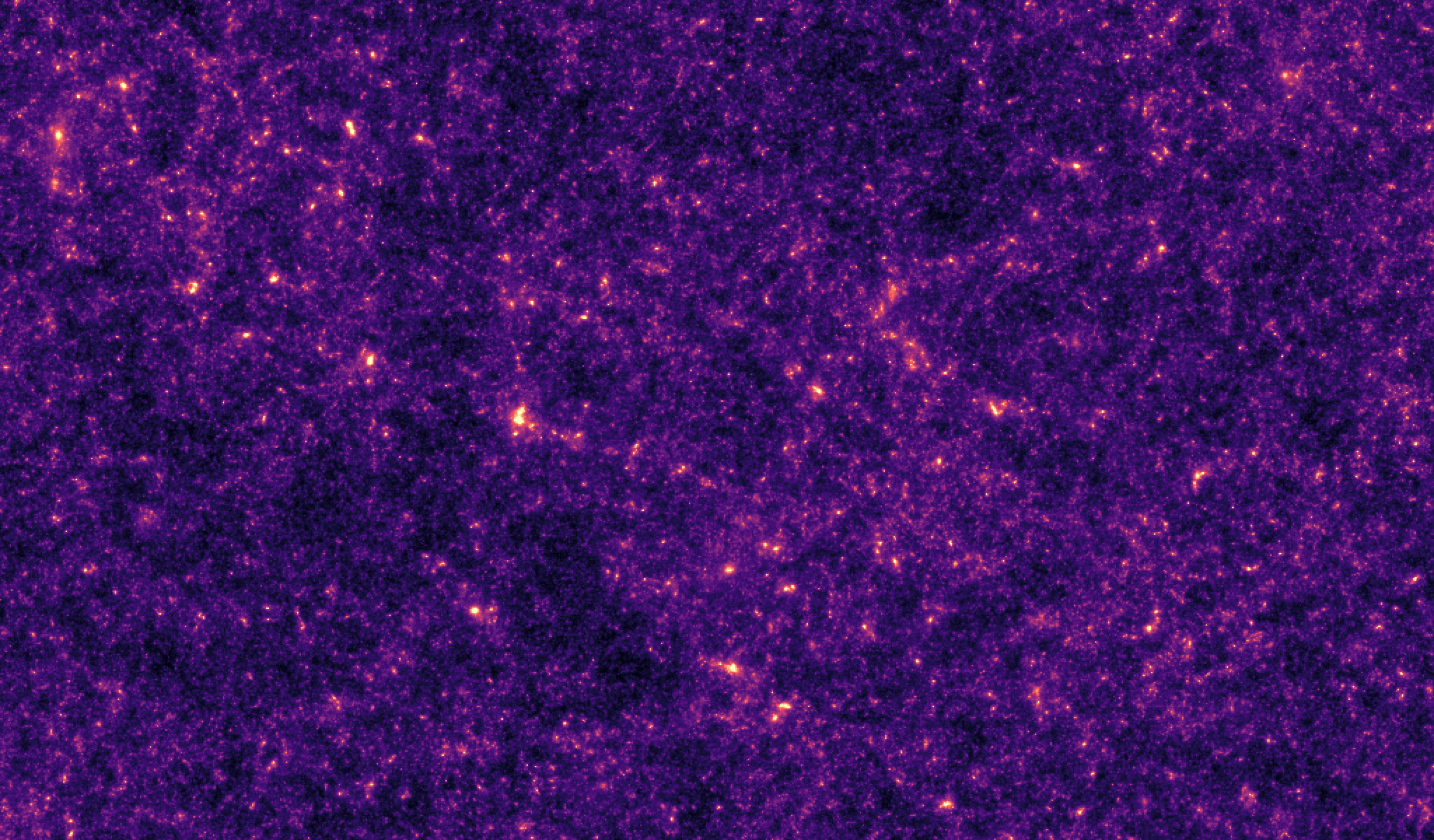
Weak Gravitational Lensing
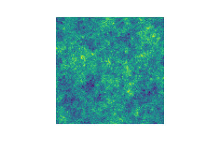
Map of the distribution of matter in the Universe.
To study dark energy we need this matter distribution at different cosmic times.
Weak Gravitational Lensing

Weak Gravitational Lensing
Weak Gravitational Lensing
Weak Gravitational Lensing
Weak Gravitational Lensing
Weak Gravitational Lensing
Weak Gravitational Lensing
Weak Gravitational Lensing
Weak Gravitational Lensing
How to constrain cosmological parameters?
For which we have an analytical likelihood function.
This likelihood function connects our compressed observations to the cosmological parameters.
Bayes theorem:
Cosmological constraints
From stage III galaxy surveys: we know it is one of the most informative of the low redshift probes.
For this reason, future surveys such as LSST, Euclid, and Roman have chosen it as their primary probe.
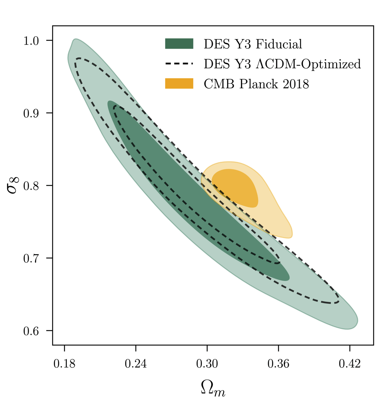

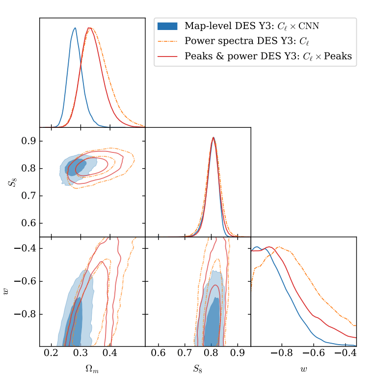
DES Y3 Results
Vera C. Rubin Observatory
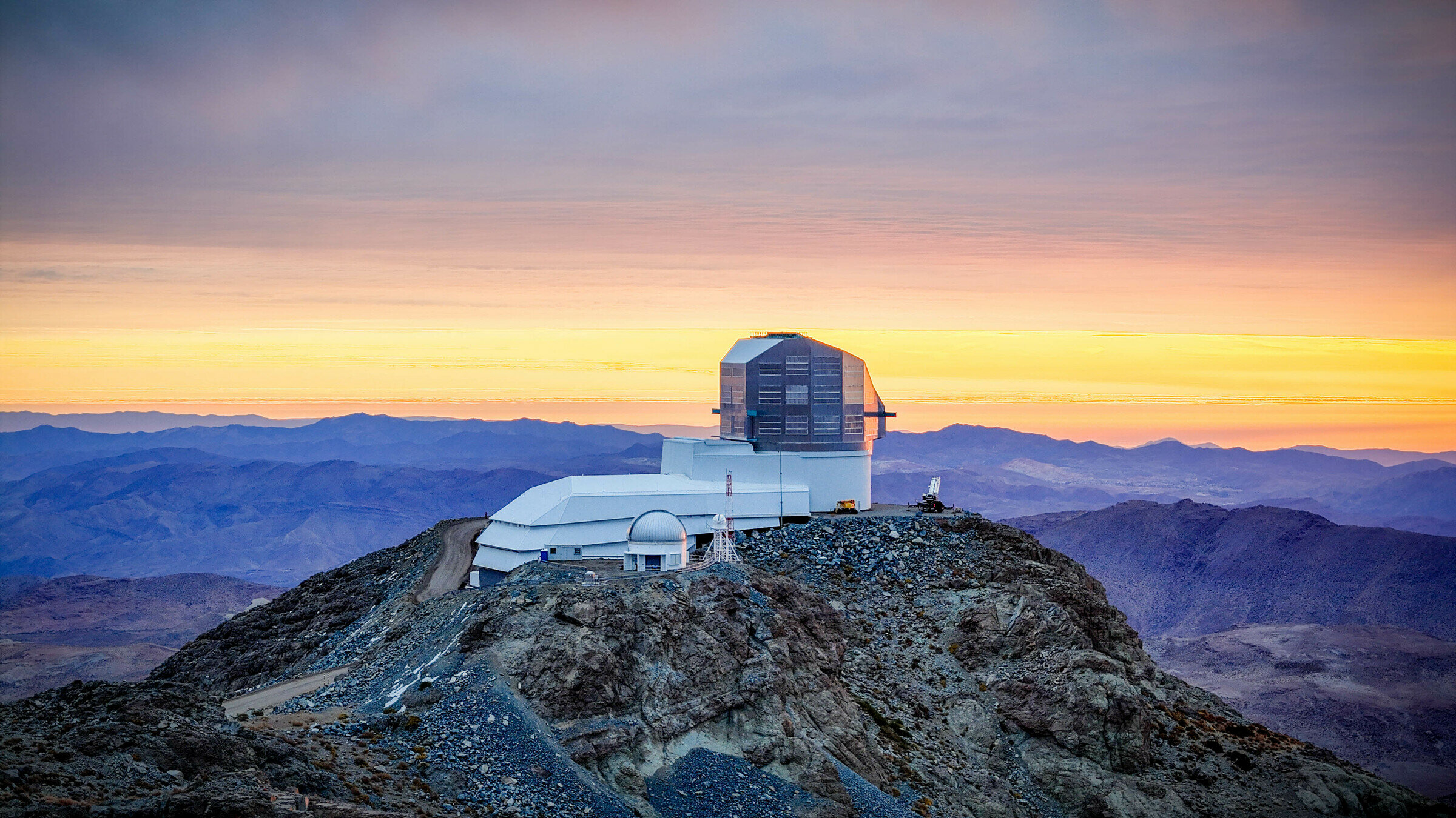
The Legacy Survey of Space and Time (LSST) will map the large-scale structure of the Universe with finer precision than ever before.
Telescope located in Chile.
It will observe the sky for 10 years taking ~1000 images every night.
Over the next 10 years, it will observe 20 billion galaxies.
Field of view: 9.6 square degrees with a pixel size of 0.2 arcsec.
We need to update our inference methods
The traditional way of constraining cosmological parameters misses information.
This results in constraints on cosmological parameters that are not precise.
Credit: Natalia Porqueres
DES Y3 Results (with SBI).
Bayes theorem:
We can build a simulator to map the cosmological parameters to the data.
Prediction
Inference
Full-field inference: extracting all cosmological information
Simulator
Full-field inference: extracting all cosmological information
Depending on the simulator’s nature we can either perform
- Explicit inference
- Implicit inference
Simulator
Full-field inference: extracting all cosmological information
-
Explicit inference
Explicit joint likelihood
Initial conditions of the Universe
Large Scale Structure
Needs an explicit simulator to sample the joint posterior through MCMC:
We need to sample in extremely
high-dimension
→ gradient-based sampling schemes.
Depending on the simulator’s nature we can either perform
- Explicit inference
- Implicit inference
Full-field inference: extracting all cosmological information
Simulator
-
Implicit inference
It does not matter if the simulator is explicit or implicit because all we need are simulations
This approach typically involve 2 steps:
2) Implicit inference on these summary statistics to approximate the posterior.
1) compression of the high dimensional data into summary statistics. Without loosing cosmological information!
Summary statistics
Full-field inference: extracting all cosmological information
Simulator
My contributions
All the work of this thesis aims to contribute to making
full-field inference applicable to next-generation surveys.
-
Which full-field inference methods require the fewest simulations?
-
How to build sufficient statistics?
-
Can we perform implicit inference with fewer simulations?
Summary statistics
Simulator
My contributions
Summary statistics
Simulator
My contributions
1. A new implicit inference method with fewer simulations.
Zeghal et al. (2022)
Summary statistics
Simulator
My contributions
1. A new implicit inference method with fewer simulations.
2. Benchmarking simulation-based inference for full-field inference.
Zeghal et al. (2022)
Zeghal et al. (2024)
Summary statistics
Simulator
3. Benchmarking neural compression for implicit full-field inference.
My contributions
1. A new implicit inference method with fewer simulations.
2. Benchmarking simulation-based inference for full-field inference.
Zeghal et al. (2022)
Zeghal et al. (2024)
Lanzieri & Zeghal et al. (2024)
Neural Posterior Estimation with Differentiable Simulators
ICML 2022 Workshop on Machine Learning for Astrophysics
Justine Zeghal, François Lanusse, Alexandre Boucaud,
Benjamin Remy and Eric Aubourg
Implicit Inference
1) Draw N parameters
2) Draw N simulations
3) Train a neural density estimator on to approximate the quantity of interest
4) Approximate the posterior from the learned quantity


Algorithm

Normalizing Flows
Normalizing Flows
Normalizing Flows
Normalizing Flows
Normalizing Flows
Normalizing Flows
Normalizing Flows
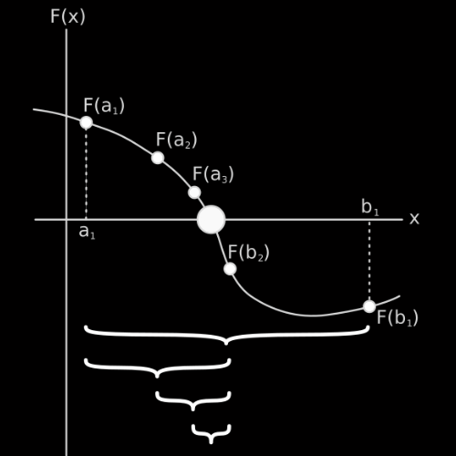
Change of Variable Formula:
Normalizing Flows
Change of Variable Formula:
Normalizing Flows
We need to learn the mapping
to approximate the complex distribution.
From simulations only!
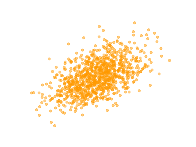
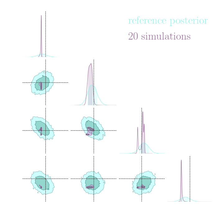
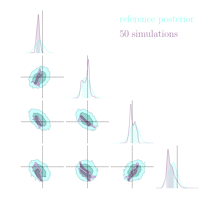
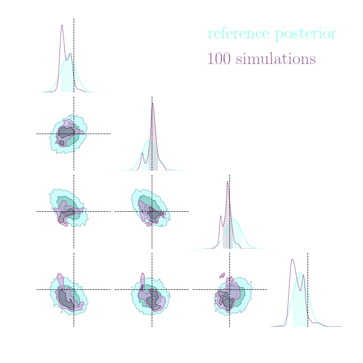
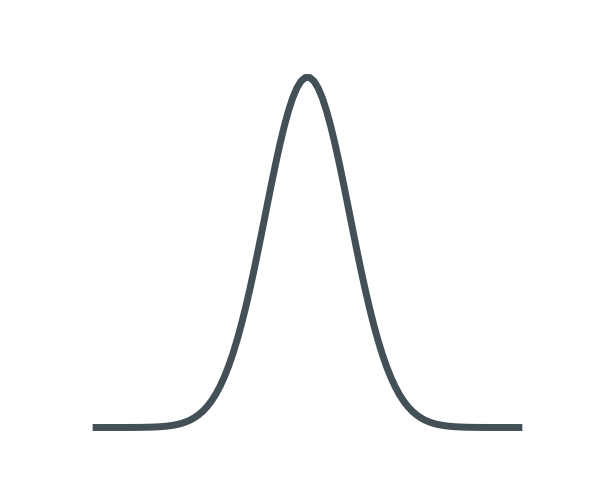
A lot of simulations..
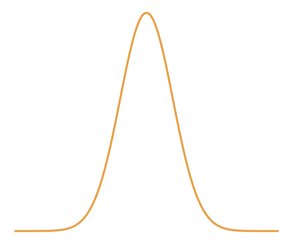
Truth
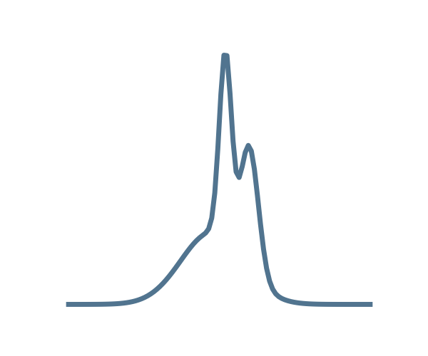
Approximation


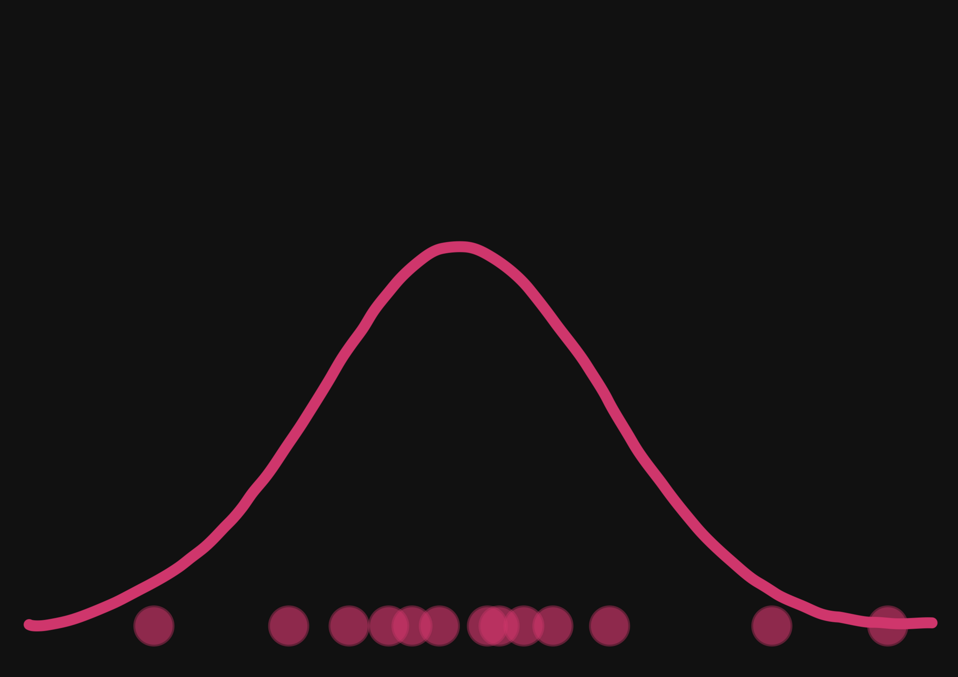
With a few simulations it's hard to approximate the posterior distribution.
→ we need more simulations
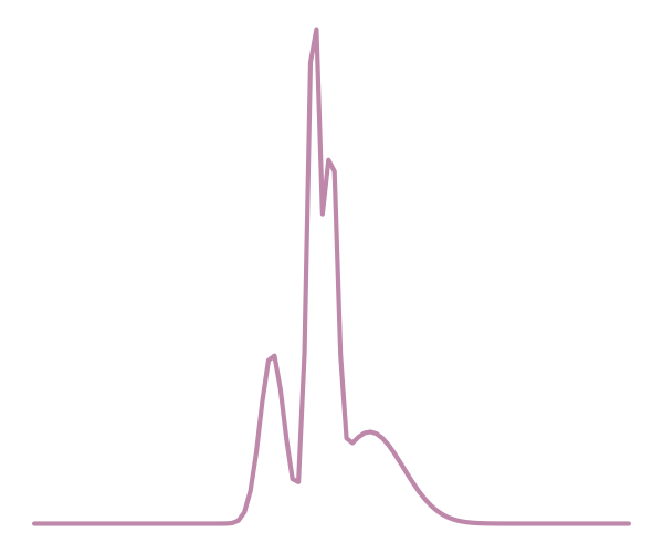
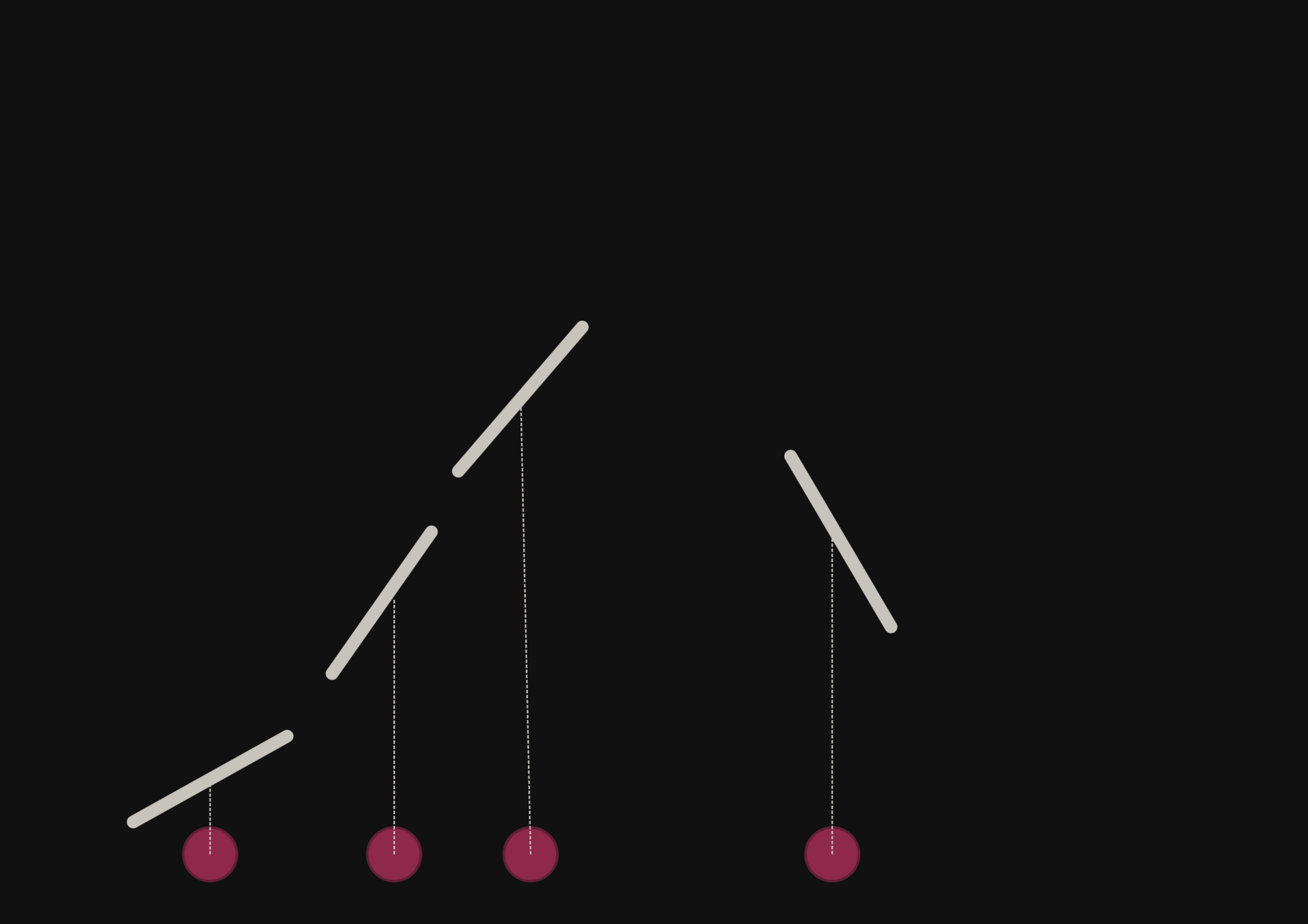
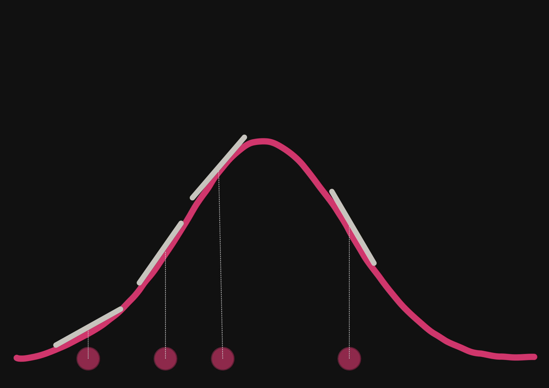
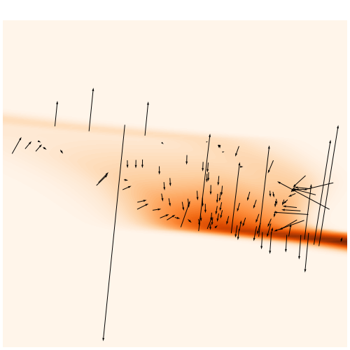
BUT if we have a few simulations
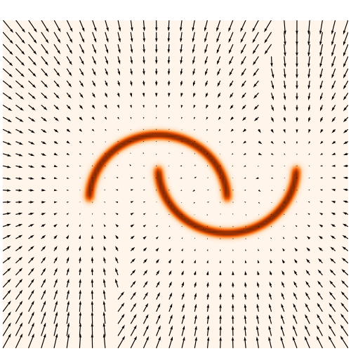
and the gradients
(also know as the score)
then it's possible to have an idea of the shape of the distribution.
How gradients can help reduce the number of simulations?
How to train NFs with gradients?
How to train NFs with gradients?
Normalizing flows are trained by minimizing the negative log likelihood:
How to train NFs with gradients?
But to train the NF, we want to use both simulations and the gradients from the simulator:
Normalizing flows are trained by minimizing the negative log likelihood:
How to train NFs with gradients?
But to train the NF, we want to use both simulations and the gradients from the simulator:
Normalizing flows are trained by minimizing the negative log likelihood:
These gradients are the joint gradients and we want to approximate
How to train NFs with gradients?
But to train the NF, we want to use both simulations and the gradients from the simulator:
Normalizing flows are trained by minimizing the negative log likelihood:
These gradients are the joint gradients and we want to approximate
How to train NFs with gradients?
But to train the NF, we want to use both simulations and the gradients from the simulator:
Normalizing flows are trained by minimizing the negative log likelihood:
These gradients are the joint gradients and we want to approximate
How to train NFs with gradients?
But to train the NF, we want to use both simulations and the gradients from the simulator:
Normalizing flows are trained by minimizing the negative log likelihood:
These gradients are the joint gradients and we want to approximate
How to train NFs with gradients?
Normalizing flows are trained by minimizing the negative log likelihood:
How to train NFs with gradients?
Normalizing flows are trained by minimizing the negative log likelihood:
Similarly to Brehmer et al., 2020, we can show that minimizing this Mean Squared Error (MSE)
How to train NFs with gradients?
Normalizing flows are trained by minimizing the negative log likelihood:
yields
Similarly to Brehmer et al., 2020, we can show that minimizing this Mean Squared Error (MSE)
How to train NFs with gradients?
Finally, the loss function that take into account simulations and gradients information is
Normalizing flows are trained by minimizing the negative log likelihood:
yields
Similarly to Brehmer et al., 2020, we can show that minimizing this Mean Squared Error (MSE)
How to train NFs with gradients?
Finally, the loss function that take into account simulations and gradients information is
Normalizing flows are trained by minimizing the negative log likelihood:
yields
Similarly to Brehmer et al., 2020, we can show that minimizing this Mean Squared Error (MSE)
How to train NFs with gradients?
How to train NFs with gradients?
Problem: the gradient of current NFs lack expressivity
How to train NFs with gradients?
Problem: the gradient of current NFs lack expressivity
How to train NFs with gradients?
Problem: the gradient of current NFs lack expressivity
How to train NFs with gradients?
Problem: the gradient of current NFs lack expressivity
How to train NFs with gradients?
Problem: the gradient of current NFs lack expressivity
→ 1cm
→ 0.01 cm
→ 0.01 cm
Benchmark Metric

A metric
We use the Classifier 2-Sample Tests (C2ST) metric.

- C2ST=0.5 (i.e “Impossible to differentiate 👍🏼”)
- C2ST=1(i.e “Too easy to differentiate 👎🏻”)
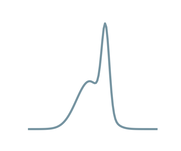
distribution 1
distribution 2
Requirement: the true distributions is needed.
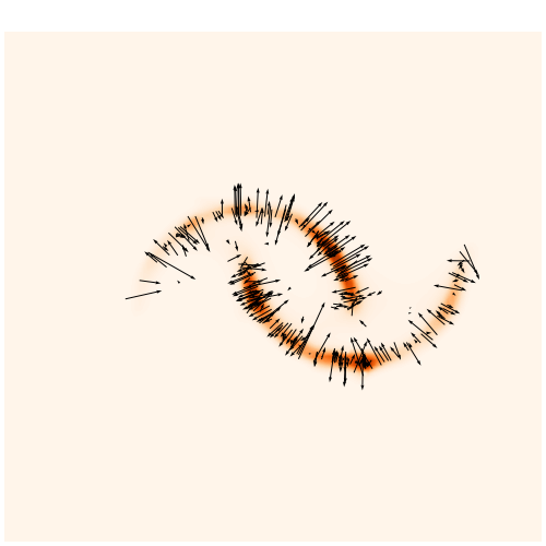
Results on a toy model

→ On a toy Lotka Volterra model, the gradients helps to constrain the distribution shape.
Results on a toy model
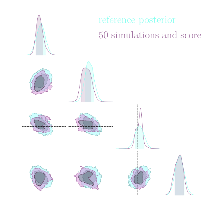
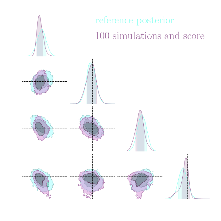
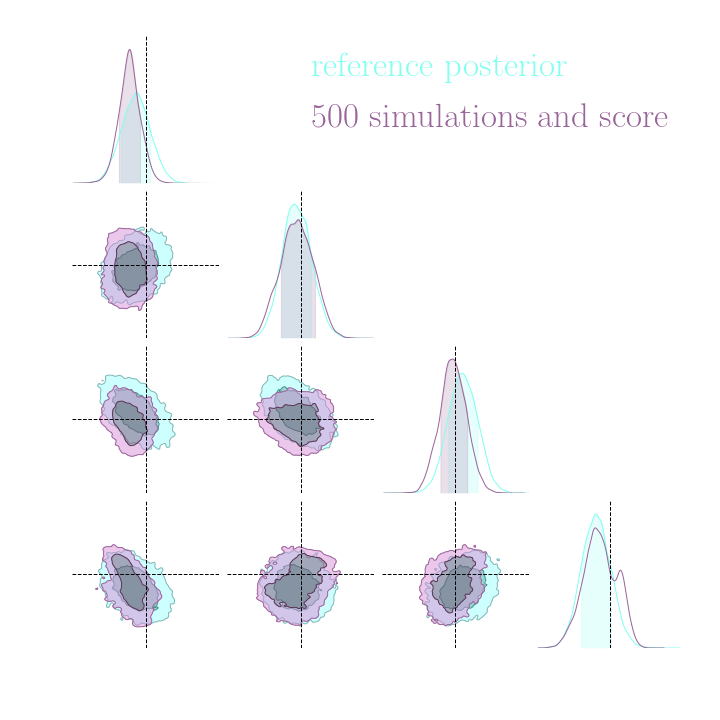
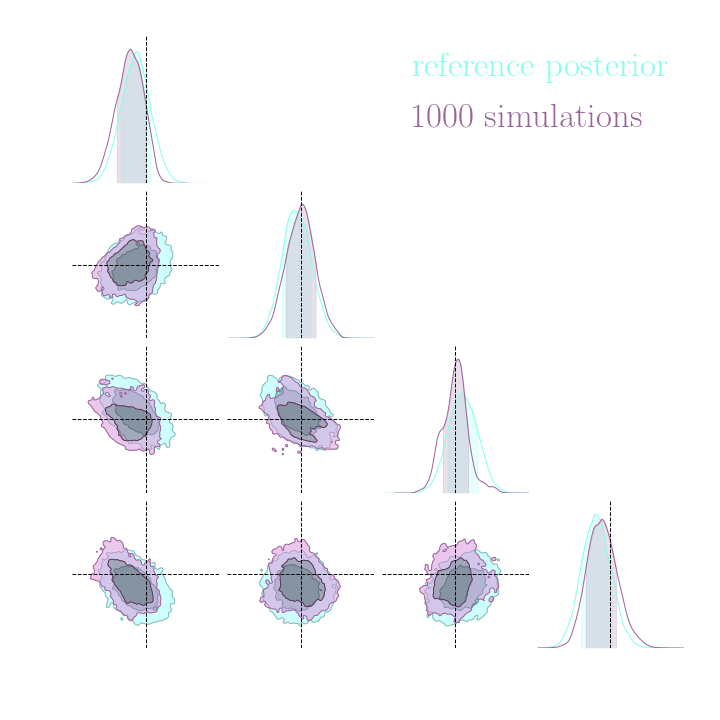
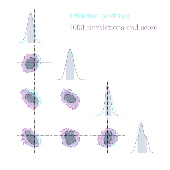
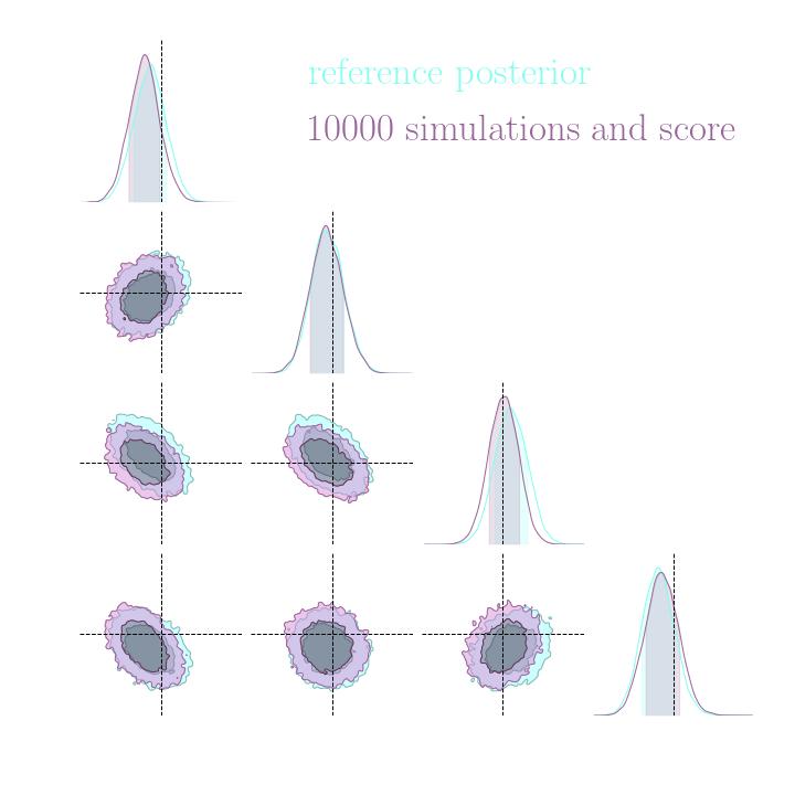
Without gradients
With gradients
Summary
First Neural Posterior Estimation (NPE) algorithm that can utilize the gradient information from the simulator.
We use an MSE loss to connect the joint gradient to the marginal one.
This loss requires the use of a specific NF architecture that is smooth.
Takeaway message
ML4Astro Workshop
Can we perform implicit inference with fewer simulations?
Yes! The gradient information helps implicit inference to reduce the number of simulations required when only a few simulations are available.
Simulator
Summary statistics
My contributions
3. Benchmarking neural compression for implicit full-field inference.
1. A new implicit inference method with fewer simulations.
2. Benchmarking simulation-based inference for full-field inference.
Zeghal et al. (2022)
Zeghal et al. (2024)
Lanzieri & Zeghal et al. (2024)
Simulation-Based Inference Benchmark for LSST Weak Lensing Cosmology
Justine Zeghal, Denise Lanzieri, François Lanusse, Alexandre Boucaud, Gilles Louppe, Eric Aubourg, Adrian E. Bayer
and The LSST Dark Energy Science Collaboration (LSST DESC)
-
do gradients help implicit inference methods?
In the case of weak lensing full-field analysis,
-
which inference method requires the fewest simulations?
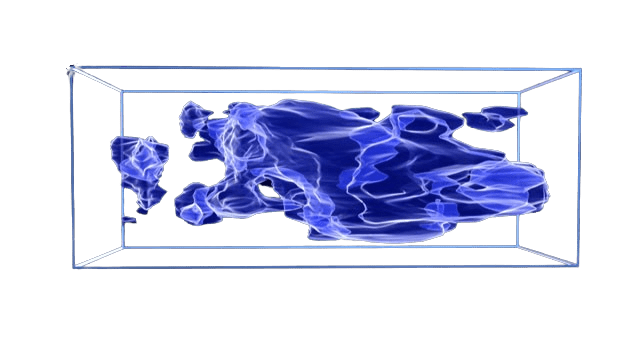
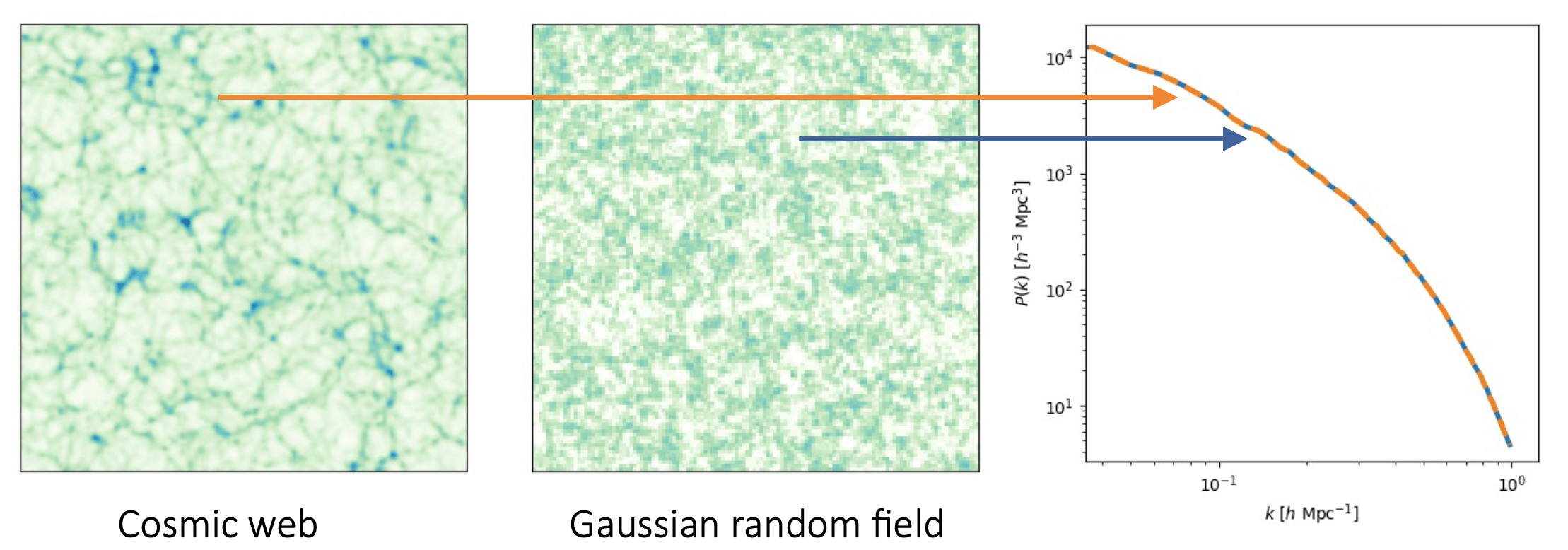
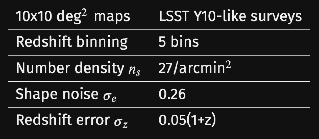
We developed a fast and differentiable (JAX) log-normal mass maps simulator.
For our benchmark: a Differentiable Mass Maps Simulator

Benchmark metric
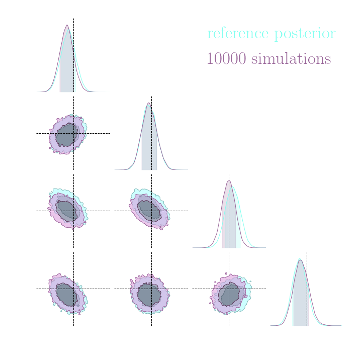
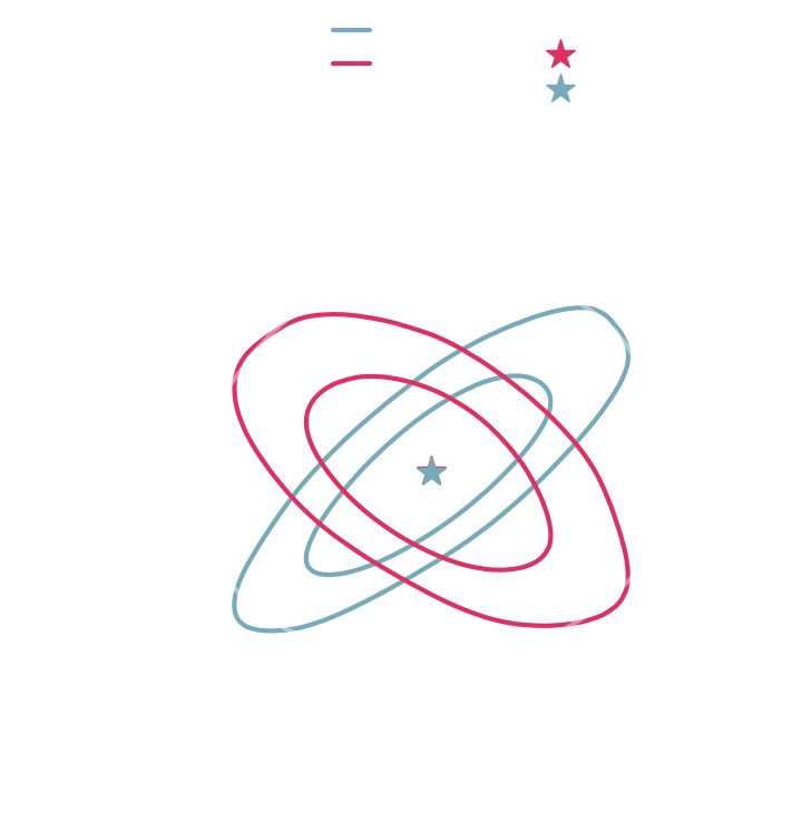
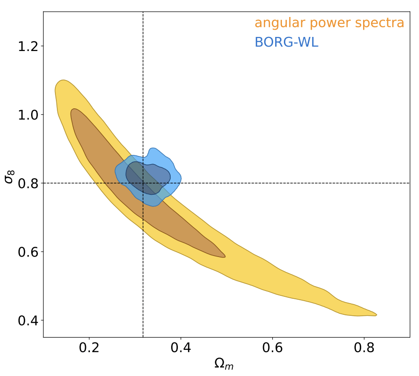
Explicit inference theoretically and asymptotically converges to the truth.
Explicit inference and implicit inference yield comparable constraints.
C2ST = 0.6!
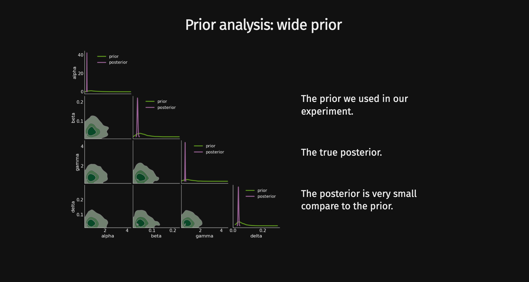
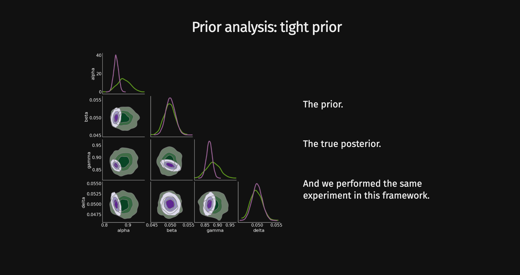
To use the C2ST we need the true posterior distribution.
→ We use the explicit full-field posterior.
Why?
-
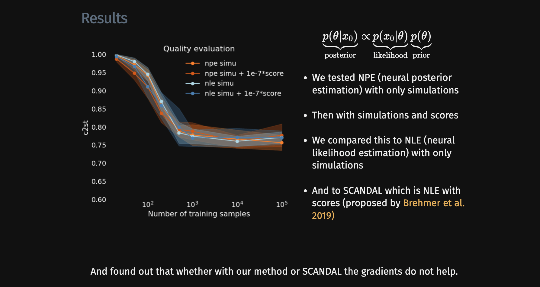
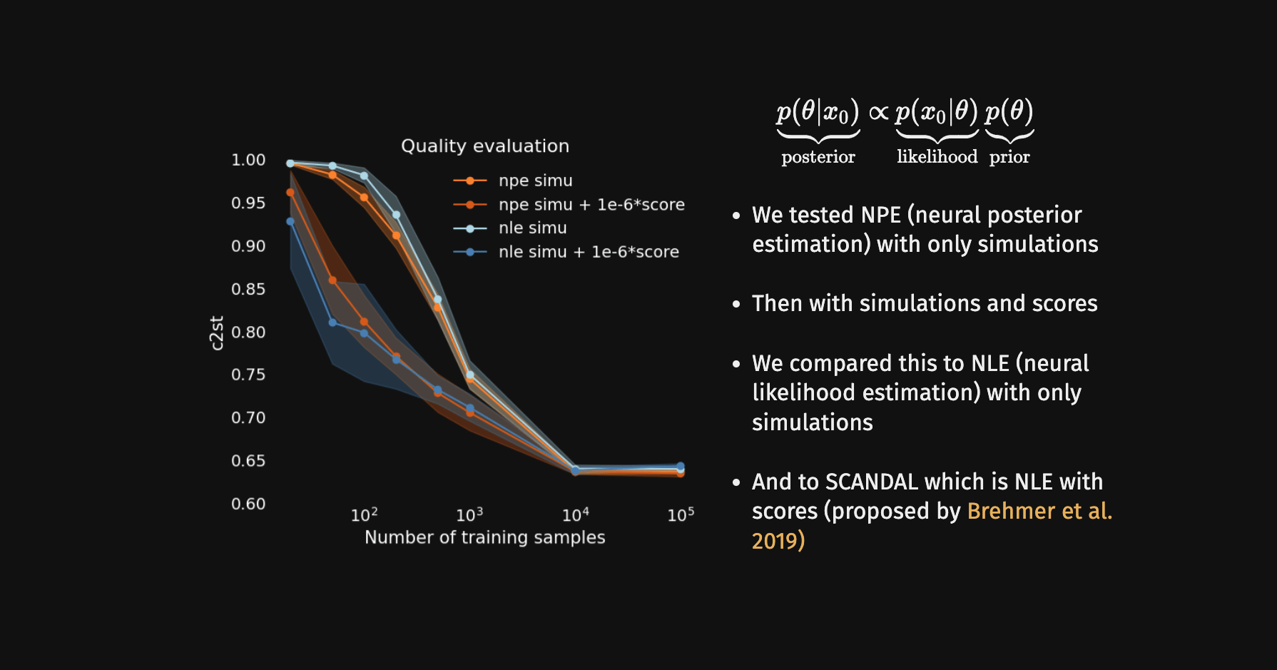
Do gradients help implicit inference methods?
Training the NF with simulations and gradients:
Loss =
-
Do gradients help implicit inference methods?

Training the NF with simulations and gradients:
Loss =
-
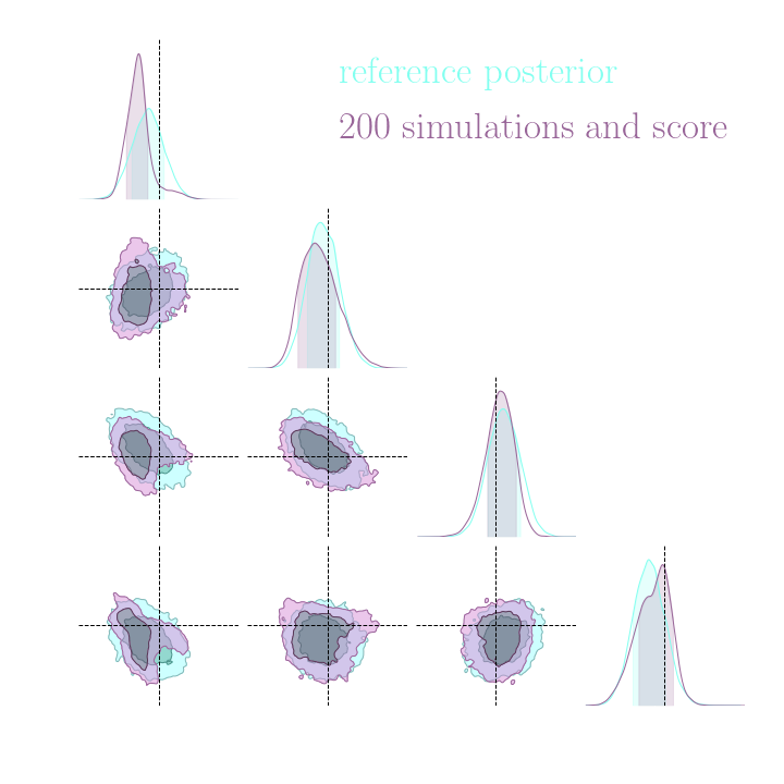
Do gradients help implicit inference methods?

(from the simulator)
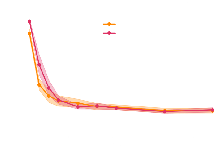
→ For this particular problem, the gradients from the simulator are too noisy to help.
-
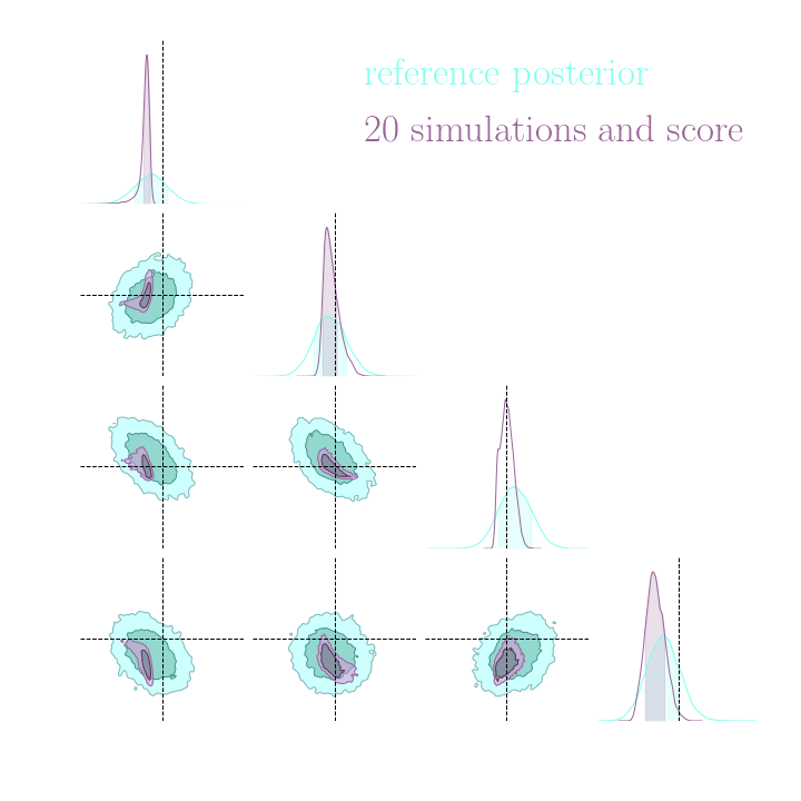
Do gradients help implicit inference methods?
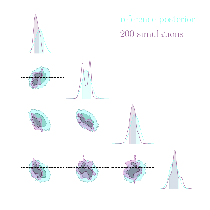
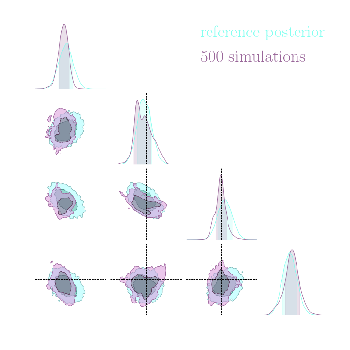
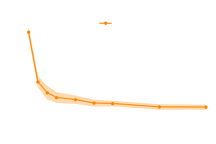
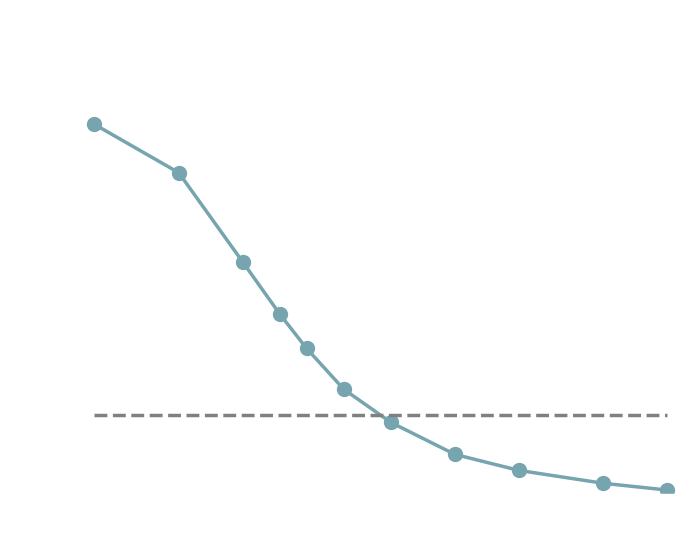
→ Implicit inference requires 1500 simulations.
→ In the case of perfect gradients it does not significantly help.
→ Simple distribution all the simulations seems to help locate the posterior distribution.
-
do gradients help implicit inference methods?
In the case of weak lensing full-field analysis,
-
which inference method requires the fewest simulations?
→ No, it does not help to reduce the number of simulations because the gradients of the simulator are too noisy.
→ Even with marginal gradients the gain is not significant.
→ For now, we now that implicit inference requires 1500 simulations.
-
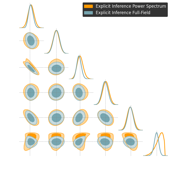
which inference method requires the fewest simulations?
What about explicit inference?
-
which inference method requires the fewest simulations?
What about explicit inference?
→ Explicit inference requires
simulations.
-
which inference method requires the fewest simulations?
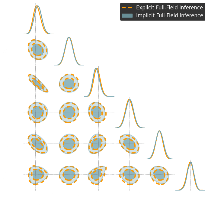
Summary
Takeaway message
Two different simulation-based inference approaches to perform full-field inference.
They yield the same constraints.
Explicit inference requires 100 times more simulations than implicit inference.
We developed a fast and differentiable log-normal simulator.
Implicit inference with gradients does not significantly help to reduce the number of simulations.
Which full-field inference methods require the fewest simulations?
Simulator
Summary statistics
My contributions
3. Benchmarking neural compression for implicit full-field inference.
1. A new implicit inference method with fewer simulations.
2. Benchmarking simulation-based inference for full-field inference.
Zeghal et al. (2022)
Zeghal et al. (2024)
Lanzieri & Zeghal et al. (2024)
Optimal Neural Summarisation for Full-Field Weak Lensing Cosmological Implicit Inference
Denise Lanzieri*, Justine Zeghal*, T. Lucas Makinen, François Lanusse, Alexandre Boucaud and Jean-Luc Starck
* equal contibutions

How to extract all the information?
It is only a matter of the loss function used to train the compressor.
Definition: Sufficient Statistic
Two main compression schemes
Regression Losses
Two main compression schemes
Text
Regression Losses
Two main compression schemes
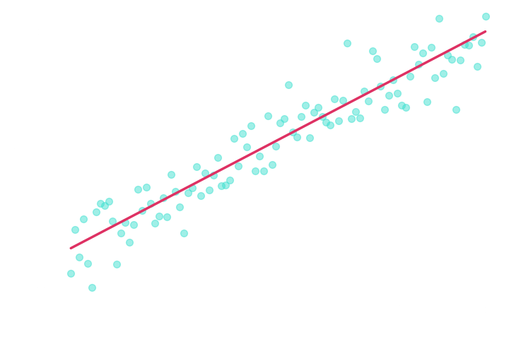
Which learns a moment of the posterior distribution.
Mean Squared Error (MSE) loss:
Which learns a moment of the posterior distribution.
Regression Losses
Two main compression schemes
Mean Squared Error (MSE) loss:
→ Approximate the mean of the posterior.
Regression Losses
Two main compression schemes
Which learns a moment of the posterior distribution.
Mean Squared Error (MSE) loss:
→ Approximate the mean of the posterior.
Regression Losses
Mean Absolute Error (MAE) loss:
Two main compression schemes
Which learns a moment of the posterior distribution.
Mean Squared Error (MSE) loss:
→ Approximate the mean of the posterior.
Regression Losses
Mean Absolute Error (MAE) loss:
→ Approximate the median of the posterior.
Two main compression schemes
Which learns a moment of the posterior distribution.
Regression Losses
Two main compression schemes
Regression Losses
Two main compression schemes
Regression Losses
Two main compression schemes
Regression Losses
Two main compression schemes
Regression Losses
The mean is not guaranteed to be a sufficient statistic.
Two main compression schemes
Mutual information maximization
Two main compression schemes
Mutual information maximization
By definition:
Two main compression schemes
Mutual information maximization
By definition:
Two main compression schemes
Mutual information maximization
By definition:
Two main compression schemes
Mutual information maximization
By definition:
Two main compression schemes
Mutual information maximization
By definition:
Two main compression schemes
Mutual information maximization
By definition:
Two main compression schemes
→ should build sufficient statistics according to the definition.
Mutual information maximization
By definition:
Two main compression schemes
For our benchmark
Log-normal LSST Y10 like
differentiable
simulator
1. We compress using one of the losses.
Benchmark procedure:
2. We compare their extraction power by comparing their posteriors.
For this, we use implicit inference, which is fixed for all the compression strategies.
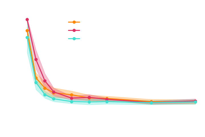
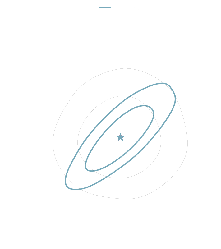
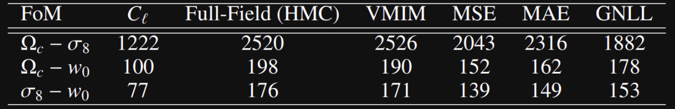
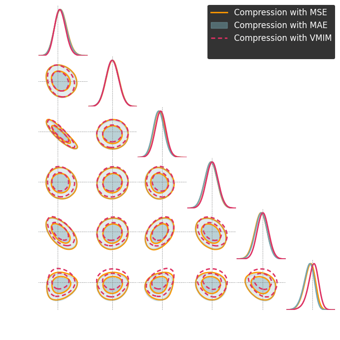
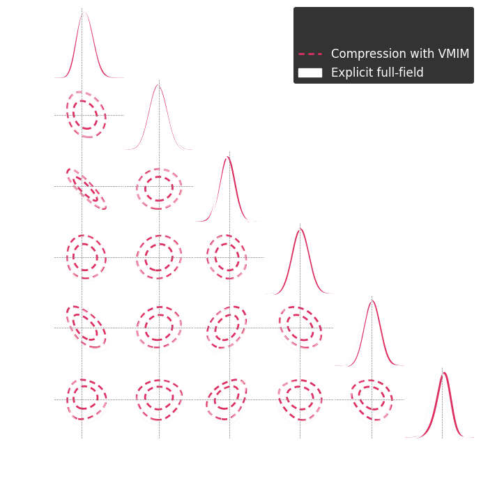
Numerical results
Summary
Takeaway message
Compression is the first step of the two-stage implicit full-field inference approach.
To perform implicit full-field inference this compression has to extract all cosmological information.
How to build sufficient statistics?
Compression schemes based on maximizing mutual information can generate sufficient statistics, while compression schemes based on regression losses do not guarantee the generation of such statistics.
Design an experimental setup that enables the isolation of the impact of the loss function.
In recent years, there has been a shift from analytical likelihood-based to simulation-based inference to enhance the precision of constraints on cosmological parameters.
Conclusion
The goal of my thesis was to conduct a cutting-edge methodological study focused on enhancing both performance (the amount of information extracted) and efficiency (the number of simulations required).
I demonstrated that achieving near-optimal implicit full-field inference is possible with just a few simulations.
Open challenges..
For instance, the fidelity of the simulator.
- Corrected the simulator with variational inference.
- Modeling the impact of baryons.
Simulator
Summary statistics
Thank you for your attention!
Backup
Coupling flows
Combine multiple mappings
Smooth Normalizing Flows
Smooth diffeomorphism (Köhler et al. (2021a)):
This function is not very expressive but a mixture of this transformation is.
Mixture of 5 transformations.
Inversing Smooth Transformations
We define as an implicit function:
and use a root-finding algorithm.
Inversing Smooth Transformations
Using automatic differentiation requires storing the value of each iteration and its gradient.
→ Inefficient.
From the Implicit Function Theorem:
Perspectives
→ Quality of inference solely tied to the simulator's quality. Realistic simulations are costly.
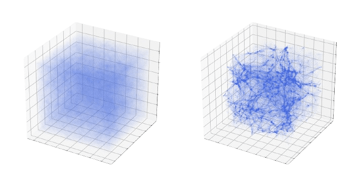
State-of-the-art explicit full-field inference results are performed on a 1LPT model.
We need a more realistic gravity model, but are we able to sample it?
Project with: Yuuki Omori, Chihway Chang, and François Lanusse.
Porqueres et al. (2023)
Perspectives
→ Quality of inference solely tied to the simulator's quality. Realistic simulations are costly.
Project with: François Lanusse, Benjamin Remy, and Alexandre Boucaud.
Even the most accurate simulations will never perfectly match our data.
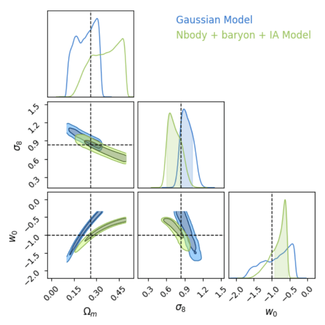
We learn the mapping between simulations and real data.
Explicit joint likelihood
Extracting gradient information
Explicit joint likelihood
Extracting gradient information
Explicit joint likelihood
Extracting gradient information
Explicit joint likelihood
Extracting gradient information

a framework for automatic differentiation following the NumPy API, and using GPU
probabilistic programming library
powered by JAX
Explicit joint likelihood
Extracting gradient information