Simulation-Based Inference for Precision Cosmology

Every Pixel Counts!

Justine Zeghal

Mila, Université de Montréal

PIML workshop 2026, Heraklion, Crete, Greece

Why do we need SBI in cosmology?

Why do we need SBI in cosmology?

Goal: Get the value of the cosmological parameters
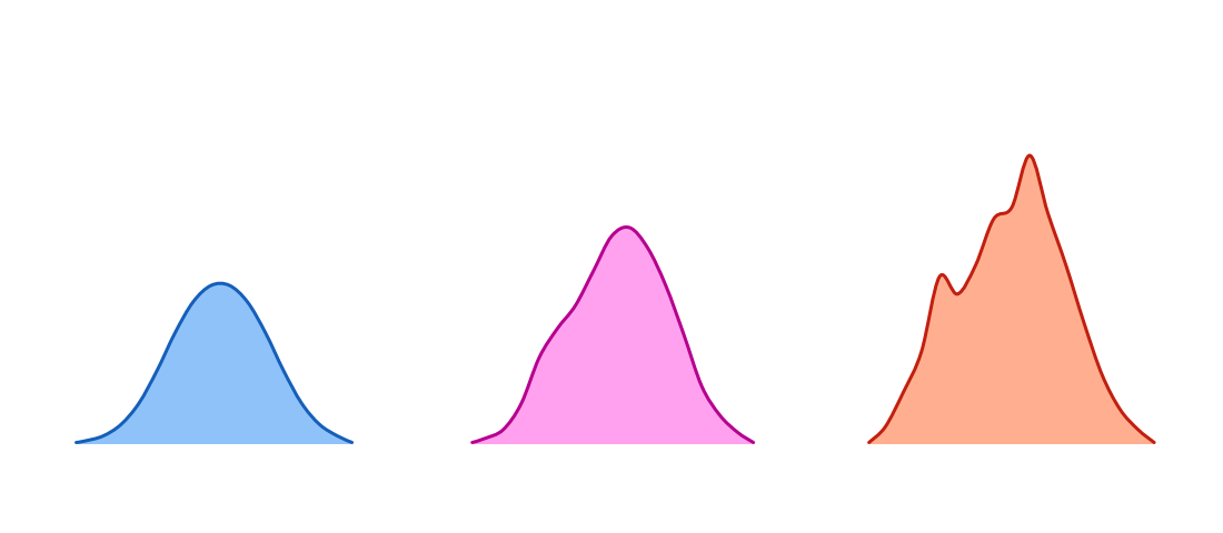
p(\theta \mid x_0)

with the uncertainty!

x_0
\Omega_c,\: \Omega_b,\:\Omega_\Lambda,\: h_0, \: n_s, \sigma_8,\: w_0
\theta
\theta
\underbrace{p(\theta|x=x_0)}_{\text{posterior}}
\underbrace{p(\theta)}_{\text{prior}}
\underbrace{p(x = x_0|\theta)}_{\text{likelihood}}
\propto

Bayes theorem:

\underbrace{p(x = x_0|\theta)}_{\text{likelihood}}

Why do we need SBI in cosmology?

x_0
p(\theta \mid x_0)
\theta

Why do we need SBI in cosmology?

x_0
p(\theta \mid x_0)
\theta

The power spectrum is near gaussian so we have an approximation of the likelihood

\mathcal{N}(t(x_0), \sigma) \approx p(x_0\mid\theta)
t_0 :=

Why do we need SBI in cosmology?

The power spectrum is near gaussian so we have an approximation of the likelihood
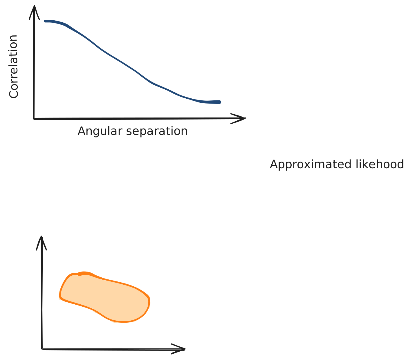
\mathcal{N}(t(x_0), \sigma) \approx p(x_0\mid\theta)

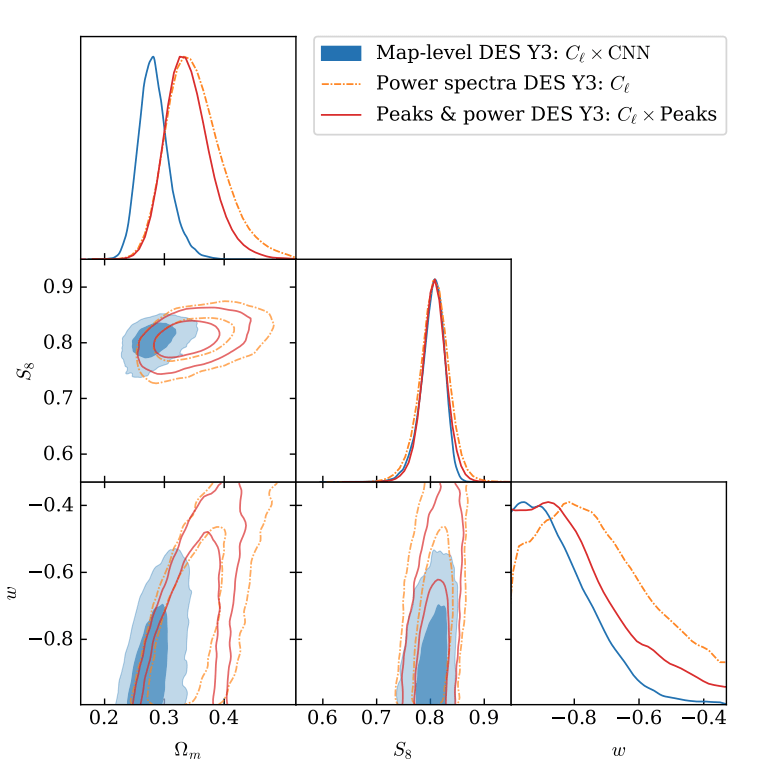
DES Y3 WL Results (with SBI).

The power spectrum is not a sufficient statistics for non gaussian field

t_0 :=

Why do we need SBI in cosmology?

Stage III

Stage IV

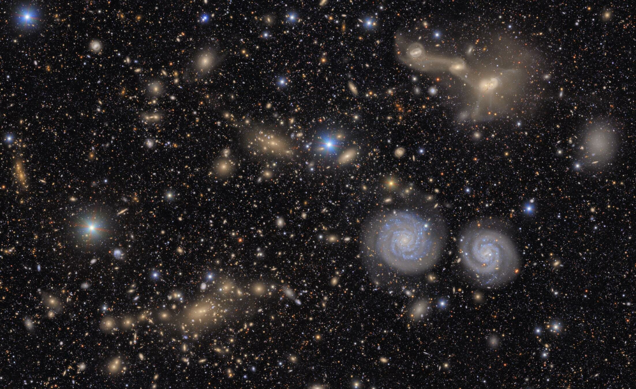
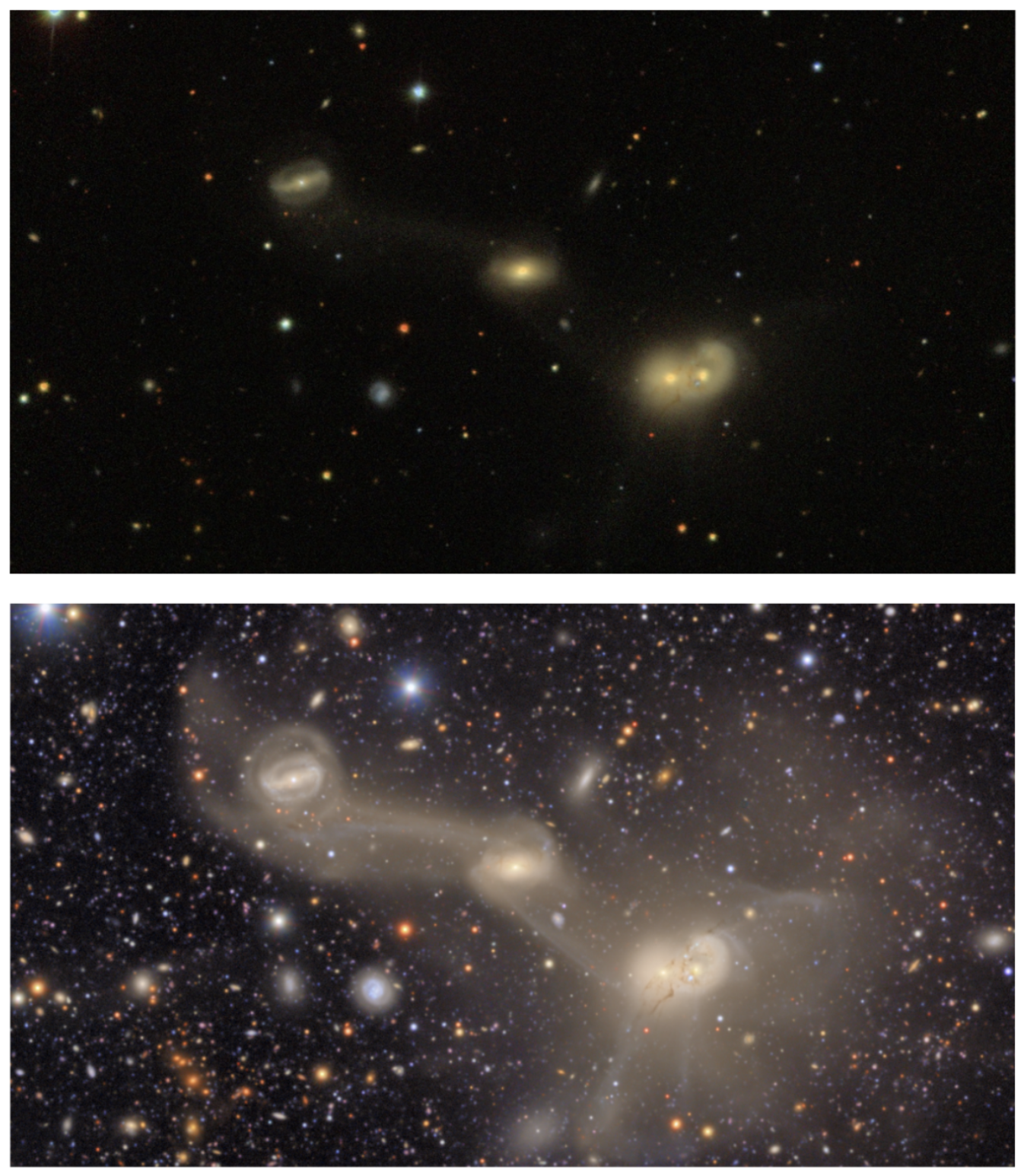
Portion of the Virgo cluster, zoom on RSCG 55

Portion of the Virgo cluster, zoom on RSCG 55

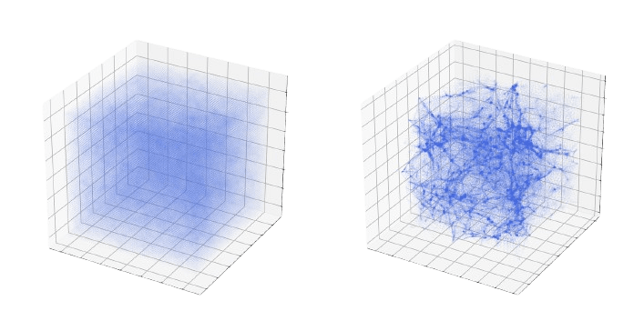
Access to new non gaussian small scales. We don't want to lose this new information!

What is SBI?

What is SBI?

What is SBI?

\theta
x
f
z_1
z_2

Simulator

z
x

Initial conditions

Large Scale Structure

\theta

Prediction

Inference

p(x| \theta, z)

Explicit inference

p(\theta, z \: | \: x) \propto
p(z\:|\:\theta) p(\theta)

Needs an explicit simulator to sample the joint posterior through MCMC:

p(x| \theta, z)
p(\theta, z \: | \: x) \propto

Implicit inference

(\theta_i, x_i)_{i=1...N}

We use simulations                                to

learn

p(\theta \mid x)

Instead of relying on an analytical model to describe the phenomenon, we can simulate it.

Two ways of performing inference from simulations:

What is SBI?

Explicit inference

p(\theta, z \: | \: x) \propto
p(z\:|\:\theta) p(\theta)

Needs an explicit simulator to sample the joint posterior through MCMC:

p(x| \theta, z)
p(\theta, z \: | \: x) \propto

Implicit inference

(\theta_i, x_i)_{i=1...N}

We use simulations                                to

learn

p(\theta \mid x)

Instead of relying on an analytical model to describe the phenomenon, we can simulate it.

Two ways of performing inference from simulations:

Because we work at the map level, considering all cosmological information, we call this inference:

Field-level inference / Pixel-level inference / Full-field inference

           Most precise inference!
How implicit inference works?

How implicit inference works?

From the dataset                                we  can learn:

(\theta_i, x_i)_{i=1...N}
p(x\mid\theta)
  • the marginal likelihood                  
p(\theta \mid x)
  • the posterior
r(x, \theta) = \frac{p(\theta \mid x)}{p(\theta)}
  • the likelihood to evidence ratio                                                            

We use generative models

Most of the time: Normalizing Flows

p_0
p_t
p_1
f^{-1}_2
f_2
f^{-1}_1
f_1

How implicit inference works?

f^{-1}_1
f^{-1}_2
f_1
f_2
p_0
p_1
p_t

How implicit inference works?

f_1
p_0
p_1
p_t

How implicit inference works?

f_1
p_0
p_1
p_t

How implicit inference works?

f_1
f_2
p_0
p_1
p_t

How implicit inference works?

f_1
f_2
f^{-1}_2
p_0
p_1
p_t

How implicit inference works?

f_1
f_2
f^{-1}_2
f^{-1}_1
p_0
p_1
p_t

How implicit inference works?

f_1
f_2
f^{-1}_2
f^{-1}_1
p_0
p_1
p_t
\log p_0(f^{-1}(x))
+ \log \displaystyle\left\lvert det \frac{\partial f^{-1}(x)}{\partial x}\right\rvert

Change of Variable Formula:

\log p_1(x)
=
f^{-1} = f_1^{-1} \circ ... \circ f_{k-1}^{-1} \circ f_k^{-1}

Should be easy to compute

We need to learn the mapping to approximate the complex distribution

How implicit inference works?

Credit: François Lanusse

 We need a tool to compare distributions:

the Kullback-Leiber Divergence

How implicit inference works?

\begin{array}{ll} D_{KL}(\color{#479af7}{p_x(x)}\color{black}{||}\color{#479af7}{p_x^{\phi}(x)}\color{black}{)} &= \mathbb{E}_{p_x(x)}\Big[ \log\left(\frac{p_x(x)}{p_x^{\phi}(x)}\right) \Big] \\ \end{array}
\begin{array}{ll} = \mathbb{E}_{p_x(x)}\left[ \log\left(p_x(x)\right) \right] \end{array}
\begin{array}{ll} - \mathbb{E}_{p_x(x)}\left[ \log\left(p_x^{\phi}(x)\right) \right]\\ \end{array}
\begin{array}{ll} = \mathbb{E}_{p_x(x)}\left[ \log\left(p_x(x)\right) \right] \end{array}
\begin{array}{ll} - \mathbb{E}_{p_x(x)}\left[ \log\left(p_x^{\phi}(x)\right) \right]\\ \end{array}

How implicit inference works?

\begin{array}{ll} D_{KL}(\color{#479af7}{p_x(x)}\color{black}{||}\color{#479af7}{p_x^{\phi}(x)}\color{black}{)} &= \mathbb{E}_{p_x(x)}\Big[ \log\left(\frac{p_x(x)}{p_x^{\phi}(x)}\right) \Big] \\ \end{array}
\begin{array}{ll} = \mathbb{E}_{p_x(x)}\left[ \log\left(p_x(x)\right) \right] \end{array}
\begin{array}{ll} - \mathbb{E}_{p_x(x)}\left[ \log\left(p_x^{\phi}(x)\right) \right]\\ \end{array}
\begin{array}{ll} = \mathbb{E}_{p_x(x)}\left[ \log\left(p_x(x)\right) \right] \end{array}
\begin{array}{ll} - \mathbb{E}_{p_x(x)}\left[ \log\left(p_x^{\phi}(x)\right) \right]\\ \end{array}
\begin{array}{ll} = \mathbb{E}_{p_x(x)}\left[ \log\left(p_x(x)\right) \right] \end{array}
\begin{array}{ll} - \mathbb{E}_{p_x(x)}\left[ \log\left(p_x^{\phi}(x)\right) \right]\\ \end{array}
\begin{array}{ll} = \mathbb{E}_{p_x(x)}\left[ \log\left(p_x(x)\right) \right] \end{array}
\begin{array}{ll} - \mathbb{E}_{p_x(x)}\left[ \log\left(p_x^{\phi}(x)\right) \right]\\ \end{array}
\phi

We want to minimize the Kullback-Leiber Divergence wrt

How implicit inference works?

\begin{array}{ll} D_{KL}(\color{#479af7}{p_x(x)}\color{black}{||}\color{#479af7}{p_x^{\phi}(x)}\color{black}{)} &= \mathbb{E}_{p_x(x)}\Big[ \log\left(\frac{p_x(x)}{p_x^{\phi}(x)}\right) \Big] \\ \end{array}
\begin{array}{ll} = \mathbb{E}_{p_x(x)}\left[ \log\left(p_x(x)\right) \right] \end{array}
\begin{array}{ll} - \mathbb{E}_{p_x(x)}\left[ \log\left(p_x^{\phi}(x)\right) \right]\\ \end{array}
\begin{array}{ll} = \mathbb{E}_{p_x(x)}\left[ \log\left(p_x(x)\right) \right] \end{array}
\begin{array}{ll} - \mathbb{E}_{p_x(x)}\left[ \log\left(p_x^{\phi}(x)\right) \right]\\ \end{array}
\begin{array}{ll} = \mathbb{E}_{p_x(x)}\left[ \log\left(p_x(x)\right) \right] \end{array}
\begin{array}{ll} - \mathbb{E}_{p_x(x)}\left[ \log\left(p_x^{\phi}(x)\right) \right]\\ \end{array}
\begin{array}{ll} = \mathbb{E}_{p_x(x)}\left[ \log\left(p_x(x)\right) \right] \end{array}
\begin{array}{ll} - \mathbb{E}_{p_x(x)}\left[ \log\left(p_x^{\phi}(x)\right) \right]\\ \end{array}
\phi

We want to minimize the Kullback-Leiber Divergence wrt

How implicit inference works?

\begin{array}{ll} D_{KL}(\color{#479af7}{p_x(x)}\color{black}{||}\color{#479af7}{p_x^{\phi}(x)}\color{black}{)} &= \mathbb{E}_{p_x(x)}\Big[ \log\left(\frac{p_x(x)}{p_x^{\phi}(x)}\right) \Big] \\ \end{array}
\begin{array}{ll} = \mathbb{E}_{p_x(x)}\left[ \log\left(p_x(x)\right) \right] \end{array}
\begin{array}{ll} - \mathbb{E}_{p_x(x)}\left[ \log\left(p_x^{\phi}(x)\right) \right]\\ \end{array}
\begin{array}{ll} = \mathbb{E}_{p_x(x)}\left[ \log\left(p_x(x)\right) \right] \end{array}
\begin{array}{ll} - \mathbb{E}_{p_x(x)}\left[ \log\left(p_x^{\phi}(x)\right) \right]\\ \end{array}
\begin{array}{ll} = \mathbb{E}_{p_x(x)}\left[ \log\left(p_x(x)\right) \right] \end{array}
\begin{array}{ll} - \mathbb{E}_{p_x(x)}\left[ \log\left(p_x^{\phi}(x)\right) \right]\\ \end{array}
= \text{constant}
\begin{array}{ll} - \mathbb{E}_{p_x(x)}\left[ \log\left(p_x^{\phi}(x)\right) \right]\\ \end{array}
\phi

We want to minimize the Kullback-Leiber Divergence wrt

How implicit inference works?

\begin{array}{ll} D_{KL}(\color{#479af7}{p_x(x)}\color{black}{||}\color{#479af7}{p_x^{\phi}(x)}\color{black}{)} &= \mathbb{E}_{p_x(x)}\Big[ \log\left(\frac{p_x(x)}{p_x^{\phi}(x)}\right) \Big] \\ \end{array}
\begin{array}{ll} = \mathbb{E}_{p_x(x)}\left[ \log\left(p_x(x)\right) \right] \end{array}
\begin{array}{ll} - \mathbb{E}_{p_x(x)}\left[ \log\left(p_x^{\phi}(x)\right) \right]\\ \end{array}
\begin{array}{ll} = \mathbb{E}_{p_x(x)}\left[ \log\left(p_x(x)\right) \right] \end{array}
\begin{array}{ll} - \mathbb{E}_{p_x(x)}\left[ \log\left(p_x^{\phi}(x)\right) \right]\\ \end{array}
\begin{array}{ll} = \mathbb{E}_{p_x(x)}\left[ \log\left(p_x(x)\right) \right] \end{array}
\begin{array}{ll} - \mathbb{E}_{p_x(x)}\left[ \log\left(p_x^{\phi}(x)\right) \right]\\ \end{array}
= \text{constant}

Simulations only!

Change of variable formula

\begin{array}{ll} \implies Loss = - \mathbb{E}_{x \sim p_x(x)}\left[ \log\left(p_x^{\phi}(x)\right) \right]\\ \end{array}
\phi

We want to minimize the Kullback-Leiber Divergence wrt

How implicit inference works?

\begin{array}{ll} \implies Loss = - \mathbb{E}_{x \sim p_x(x)}\left[ \log\left(p_x^{\phi}(x)\right) \right]\\ \end{array}

How implicit inference works?

\begin{array}{ll} Loss = - \mathbb{E}_{x, \theta \sim p(x, \theta)}\left[ \log\left(p^{\phi}(x \mid \theta)\right) \right]\\ \end{array}
\begin{array}{ll} \implies Loss = - \mathbb{E}_{x \sim p_x(x)}\left[ \log\left(p_x^{\phi}(x)\right) \right]\\ \end{array}

Likelihood approximation (e.g. Papamakarios et al., 2019)

\begin{array}{ll} \implies Loss = - \mathbb{E}_{x \sim p_x(x)}\left[ \log\left(p_x^{\phi}(x)\right) \right]\\ \end{array}

How implicit inference works?

\begin{array}{ll} Loss = - \mathbb{E}_{x, \theta \sim p(x, \theta)}\left[ \log\left(p^{\phi}(x \mid \theta)\right) \right]\\ \end{array}

Likelihood approximation (e.g. Papamakarios et al., 2019)

\begin{array}{ll} Loss = - \mathbb{E}_{x, \theta \sim p(x, \theta)}\left[ \log\left(p^{\phi}(\theta \mid x)\right) \right]\\ \end{array}

Posterior approximation (e.g. Papamakarios et al., 2016)

\begin{array}{ll} \implies Loss = - \mathbb{E}_{x \sim p_x(x)}\left[ \log\left(p_x^{\phi}(x)\right) \right]\\ \end{array}

Both methods require a lot of costly simulations!

Implicit inference with few simulations

Implicit inference with few simulations

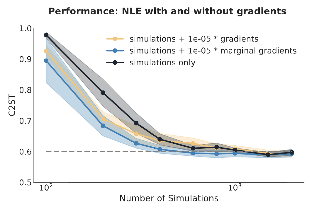
Brehmer et al. (2018), Zeghal et al. (2022)

\displaystyle \mathbb{E}\left[ \parallel \nabla_{\theta} \log p^{\phi}(\theta |x) - \nabla_{\theta} \log p(\theta, z |x)\parallel_2^2 \right]
\begin{array}{ll} Loss = - \mathbb{E}_{x, \theta \sim p(x, \theta)}\left[ \log\left(p ^{\phi}(\theta \mid x)\right) \right]\\ \end{array}

For instance for NPE:

Neural-based SBI

?

\nabla_{\theta} \log p^{\phi}(\theta |x) \approx \nabla_{\theta} \log p(\theta|x)

 We also want to use the simulator's gradients information:

\nabla_{\theta} \log p(\theta, z |x)

and we want to learn the marginal posterior but

\nabla_\theta \log p(\theta|x)
= \nabla_\theta \log \int p(\theta,z|x)dz
\color{black}{\neq \int} \color{#b6008e}{\nabla_{\theta} \log p(\theta, z |x) dz}

Minimized by

Implicit inference with few simulations

\displaystyle \mathbb{E}\left[ \parallel \nabla_{\theta} \log p^{\phi}(\theta |x) - \nabla_{\theta} \log p(\theta, z |x)\parallel_2^2 \right]
\begin{array}{ll} Loss = - \mathbb{E}_{x, \theta \sim p(x, \theta)}\left[ \log\left(p ^{\phi}(\theta \mid x)\right) \right]\\ \end{array}

Neural-based SBI

+ \lambda

Lack expressivity!

Brehmer et al. (2018), Zeghal et al. (2022)

Implicit inference with few simulations

Neural-based SBI
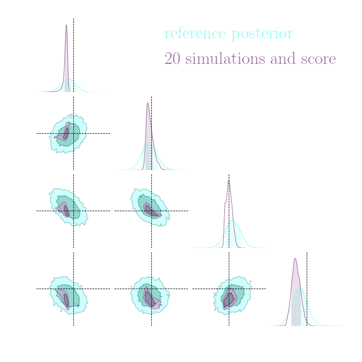
Without gradients

With gradients

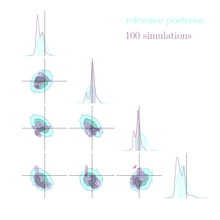
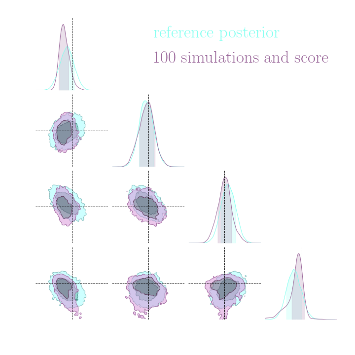
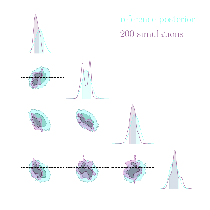
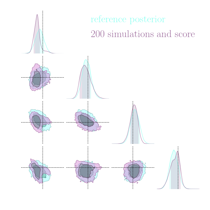
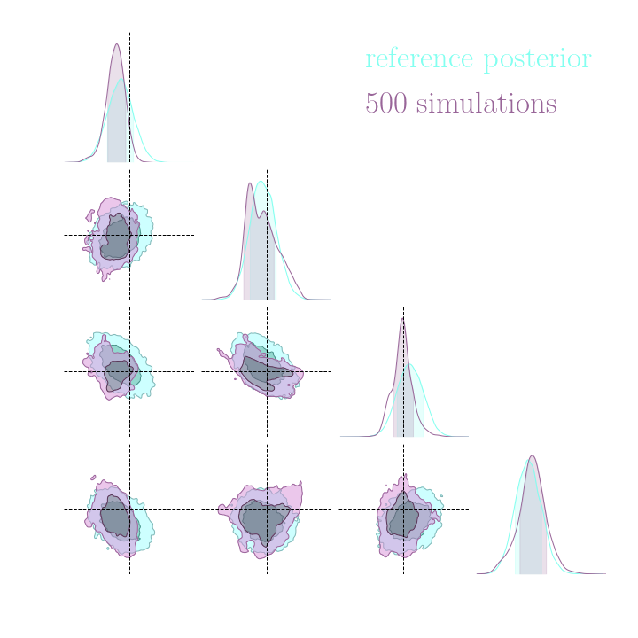
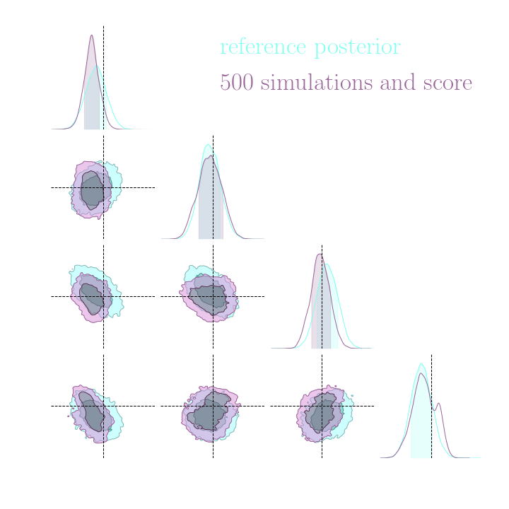
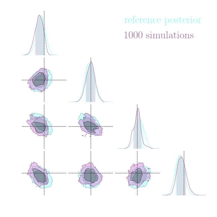
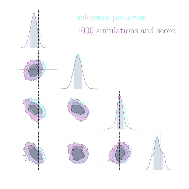
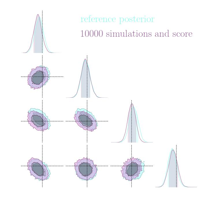
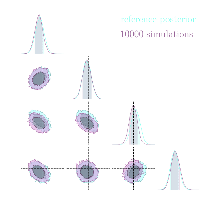
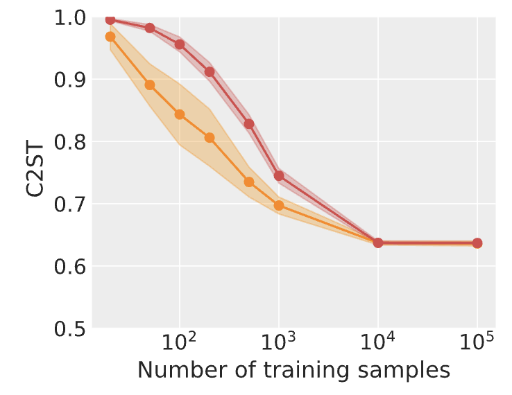
Some results

Without gradients

With gradients

Brehmer et al. (2018), Zeghal et al. (2022)

Implicit inference with few simulations

Neural-based SBI
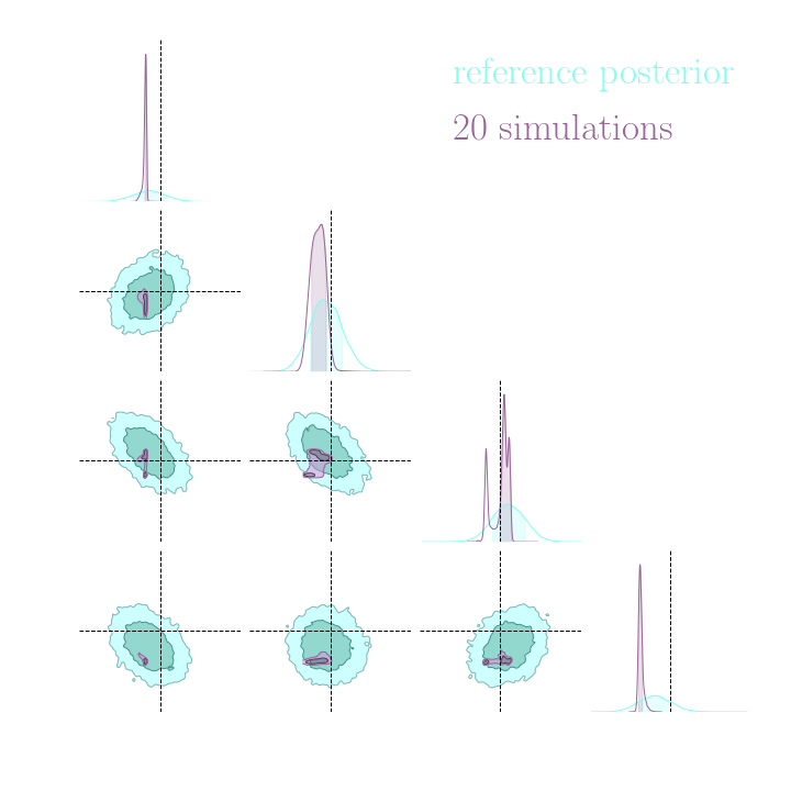
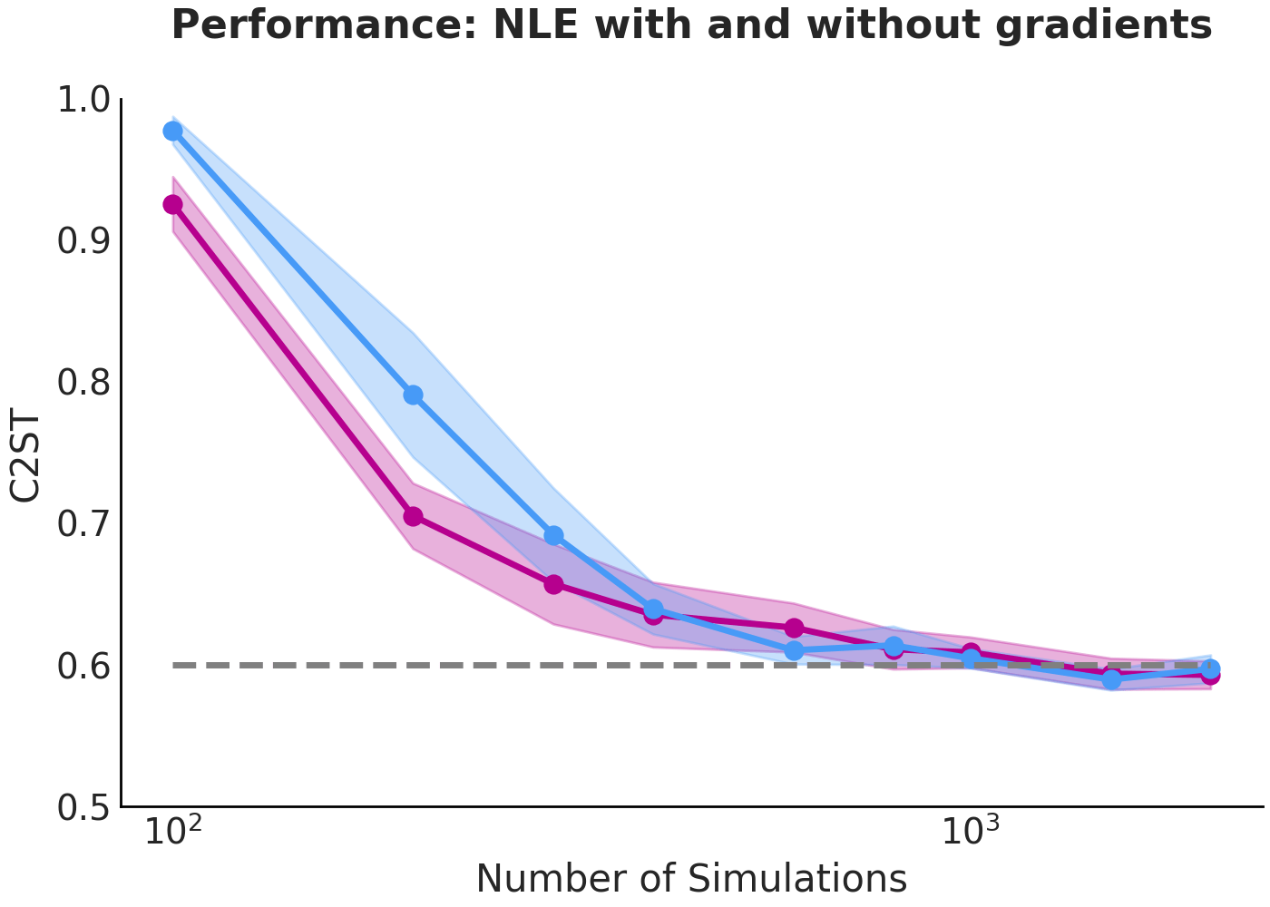
Application to Weak Lensing Cosmology

Zeghal et al. (2024)

Implicit inference with few simulations

Neural-based SBI
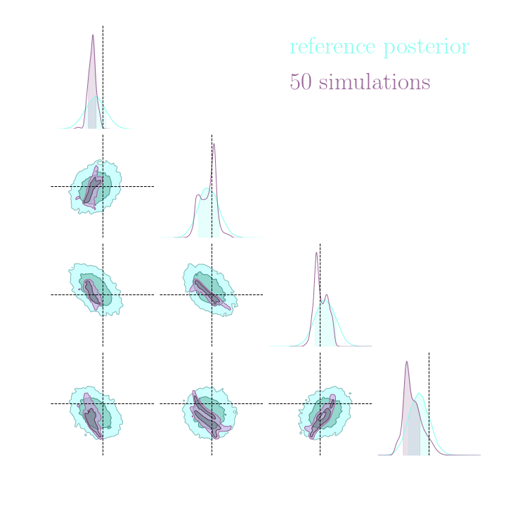
Application to Weak Lensing Cosmology

Zeghal et al. (2024)

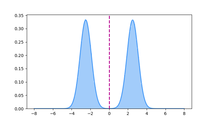
No improvements when using the gradients.
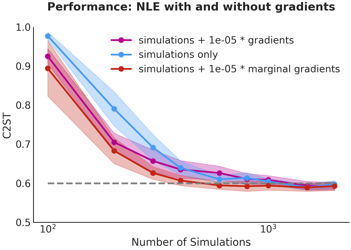
We are using the joint gradients:
\nabla_{\theta} \log p(\theta, z |x) \neq
\nabla_\theta \log p(\theta|x)

Need to check your gradients before. And maybe use variance reduction techniques.

Implicit inference with few simulations

+ \: \lambda \: \displaystyle \mathbb{E}\left[ \parallel \nabla_{\theta} \log p^{\phi}(\theta |x) - \nabla_{\theta} \log p(\theta, z |x)\parallel_2^2 \right]
\begin{array}{ll} Loss = - \mathbb{E}_{x, \theta \sim p(x, \theta)}\left[ \log\left(p ^{\phi}(\theta \mid x)\right) \right]\\ \end{array}

For instance for NPE:

Neural-based SBI

?

Lack expressivity!

Brehmer et al. (2018), Zeghal et al. (2022)

Building more simulations at low cost
Building more simulations at low cost

Building more simulations at low cost

 e.g. log-normal, LPT, PM

O(ms) runtime
differentiable  
realistic

Fast simulations

e.g. full nbody, hydro

Costly simulations

O(ms) runtime
differentiable  
realistic
f_\varphi

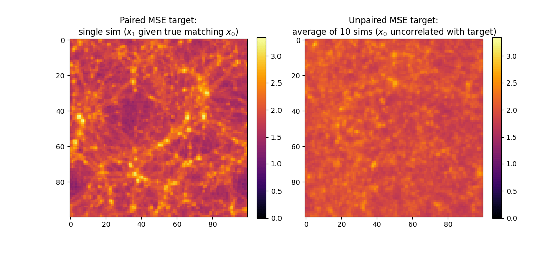
We can learn the mapping between a cheap and a realistic simulation

Easier to learn a small correction & requires fewer simulations

One way to do:

\mathbb{E}_{p(x_1,x_0)} \Big[ \| \color{#b6008e}{f_\varphi} \color{black}{(x_0)- x_1 \|^2 \Big]}

minimized by

\color{#b6008e}{f_\varphi}^* \color{black}{(x_0)=\mathbb{E}_{p(x_1\mid x_0)} [x_1] }

which is fine if, for instance                   , is a dirac

p(x_1 \mid x_0)

Building more simulations at low cost

p(x_1\mid x_0)
\color{#b6008e}{f_\varphi}^* \color{black}{(x_0)}

We can learn the mapping between a cheap and a realistic simulation

Easier to learn a small correction & requires fewer simulations

One way to do:

\mathbb{E}_{p(x_1,x_0)} \Big[ \| \color{#b6008e}{f_\varphi} \color{black}{(x_0)- x_1 \|^2 \Big]}

minimized by

\color{#b6008e}{f_\varphi}^* \color{black}{(x_0)=\mathbb{E}_{p(x_1\mid x_0)} [x_1] }

which is fine if, for instance                   , is a dirac

p(x_1 \mid x_0)

Building more simulations at low cost

Building more simulations at low cost

We can learn the mapping between a cheap and a realistic simulation

Easier to learn a small correction & requires fewer simulations

One way to do:

\mathbb{E}_{p(x_1,x_0)} \Big[ \| \color{#b6008e}{f_\varphi} \color{black}{(x_0)- x_1 \|^2 \Big]}

minimized by

\color{#b6008e}{f_\varphi}^* \color{black}{(x_0)=\mathbb{E}_{p(x_1\mid x_0)} [x_1] }

which is fine if, for instance                   , is a dirac

p(x_1 \mid x_0)
p(x_1\mid x_0)
\color{#b6008e}{f_\varphi}^* \color{black}{(x_0)}
p(x_1\mid x_0)
x_1 \sim p(x_1)

when                    is not a dirac we should use generative models to get probable samples

Building more simulations at low cost

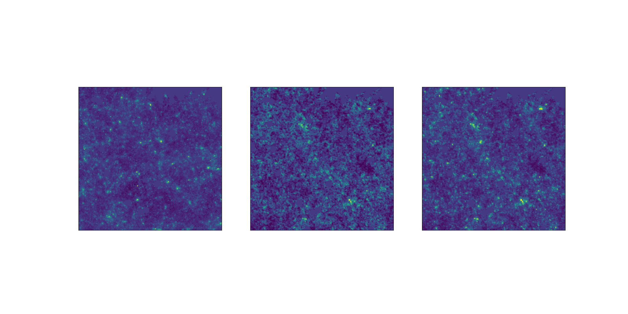
For instance, in Zeghal et al. (2025) we aim to approximate

p(x_1\mid \theta)

from unpaired simulations

  •                   is not a dirac
p(x_1 \mid x_0)
  • how to benefit from the approximate simulations?
Dataset 2

x^D_1
x^E_1
x^F_1
\theta^D
\theta^E
\theta^F

Dataset 1

x^A_0
x^B_0
x^C_0
\theta^A
\theta^B
\theta^C

unlearning dataset 1 would requires more simulations than starting from gaussian noise

Conditional Optimal Transport Flow Macthing (Kerrigan et al. 2024)

Building more simulations at low cost

Conditional Optimal Transport Flow Macthing (Kerrigan et al. 2024)

Building more simulations at low cost

p_0
p_1
p_t

We need to learn a continuous transformation      solution of the ODE

f_t
\frac{d x}{dt} = \color{#479af7}{v}\color{black}{(x, t)}

velocity field

More flexible!

Conditional Optimal Transport Flow Macthing (Kerrigan et al. 2024)

Building more simulations at low cost

\frac{d x}{dt} = \color{#479af7}{v}\color{black}{(x, t)}

Conditional Optimal Transport Flow Macthing (Kerrigan et al. 2024)

Building more simulations at low cost

\frac{d x}{dt} = \color{#479af7}{v}\color{black}{(x, t)}

Conditional Optimal Transport Flow Macthing (Kerrigan et al. 2024)

Building more simulations at low cost

\mathcal{L}_{FM} = \mathbb{E}_{p(t)q(x_0,x_1)p_t(x_t\mid x_0,x_1)} \Big[ \| \color{#b6008e}{v_\varphi} \color{black}{(x_t,t)- v(x_t) \|^2 \Big]}

Lipman et al. (2023)

\frac{d x}{dt} = \color{#479af7}{v}\color{black}{(x, t)}

Conditional Optimal Transport Flow Macthing (Kerrigan et al. 2024)

Building more simulations at low cost

Lipman et al. (2023)

\frac{d x}{dt} = \color{#479af7}{v}\color{black}{(x, t)}

Conditional Optimal Transport Flow Macthing (Kerrigan et al. 2024)

\mathcal{L}_{FM} = \mathbb{E}_{p(t)q(x_0,x_1)p_t(x_t\mid x_0,x_1)} \Big[ \| \color{#b6008e}{v_\varphi} \color{black}{(x_t,t)- v(x_t|x_0,x_1) \|^2 \Big]}

Building more simulations at low cost

Lipman et al. (2023)

\frac{d x}{dt} = \color{#479af7}{v}\color{black}{(x, t)}

Conditional Optimal Transport Flow Macthing (Kerrigan et al. 2024)

\mathcal{L}_{FM} = \mathbb{E}_{p(t)q(x_0,x_1)p_t(x_t\mid x_0,x_1)} \Big[ \| \color{#b6008e}{v_\varphi} \color{black}{(x_t,t)- v(x_t|x_0,x_1) \|^2 \Big]}
p(x_t\mid x_0,x_1) = \mathcal{N}((1-t)x_1 + t x_0, \sigma)
v(x_t| x_0,x_1) = x_1 - x_0

with:

Tong et al. 2023

Building more simulations at low cost

\frac{d x}{dt} = \color{#479af7}{v}\color{black}{(x, t)}

Conditional Optimal Transport Flow Macthing (Kerrigan et al. 2024)

\mathcal{L}_{FM} = \mathbb{E}_{p(t)q(x_0,x_1)p_t(x_t\mid x_0,x_1)} \Big[ \| \color{#b6008e}{v_\varphi} \color{black}{(x_t,t)- v(x_t|x_0,x_1) \|^2 \Big]}
p(x_t\mid x_0,x_1) = \mathcal{N}((1-t)x_1 + t x_0, \sigma)
v(x_t| x_0,x_1) = x_1 - x_0

with:

Tong et al. 2023

  • Continuous transformation + simulation-free training: high dimension ✅
  • Interpolants framework: arbitrary source distribution ✅

Building more simulations at low cost
Conditional Optimal Transport Flow Macthing (Kerrigan et al. 2024)

  • Continuous transformation + simulation-free training: high dimension ✅
  • Interpolants framework: arbitrary source distribution ✅

Unlearning dataset 1 would requires more simulations than starting from gaussian noise

OT to find the minimal effort mapping

Building more simulations at low cost
Conditional Optimal Transport Flow Macthing (Kerrigan et al. 2024)

  • Continuous transformation + simulation-free training: high dimension ✅
  • Interpolants framework: arbitrary source distribution ✅

Unlearning dataset 1 would requires more simulations than starting from gaussian noise

OT to find the minimal effort mapping

Building more simulations at low cost

Conditional Optimal Transport Flow Macthing (Kerrigan et al. 2024)

  • Continuous transformation + simulation-free training: high dimension ✅
  • Interpolants framework: arbitrary source distribution ✅

Unlearning dataset 1 would requires more simulations than starting from gaussian noise

OT to find the minimal effort mapping

Building more simulations at low cost

Conditional Optimal Transport Flow Macthing (Kerrigan et al. 2024)

  • Continuous transformation + simulation-free training: high dimension ✅
  • Interpolants framework: arbitrary source distribution ✅

Unlearning dataset 1 would requires more simulations than starting from gaussian noise

OT to find the minimal effort mapping

Building more simulations at low cost

Conditional Optimal Transport Flow Macthing (Kerrigan et al. 2024)

x^A_0
x^D_1

Building more simulations at low cost

Conditional Optimal Transport Flow Macthing (Kerrigan et al. 2024)

x^D_1
x^E_1
x^F_1

OT will find the "closest" map!

x^A_0

Building more simulations at low cost

Conditional Optimal Transport Flow Macthing (Kerrigan et al. 2024)

x^E_1

x^A_0

Building more simulations at low cost

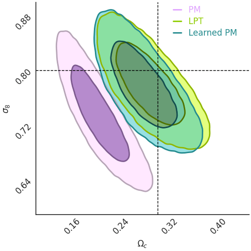
Zeghal et al. (2025)

p_{\text{cheap}}(\theta \mid x_{\text{cheap}} = x_{\text{realistic}})
p_{\text{realistic}}(\theta \mid x_{\text{realistic}} = x_{\text{realistic}})
p_{\text{emulated}}(\theta \mid x_{\text{emulated}} = x_{\text{realistic}})

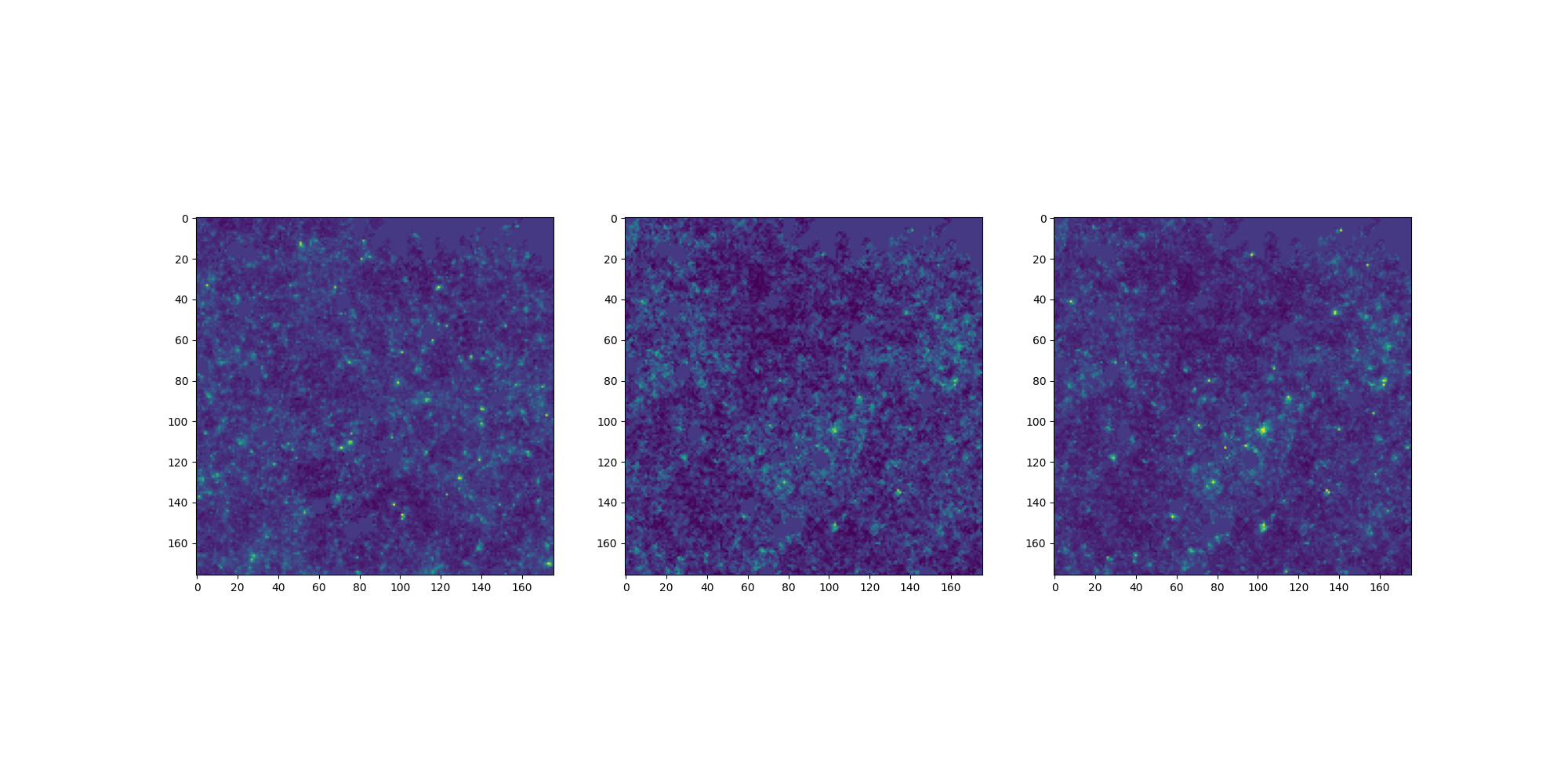
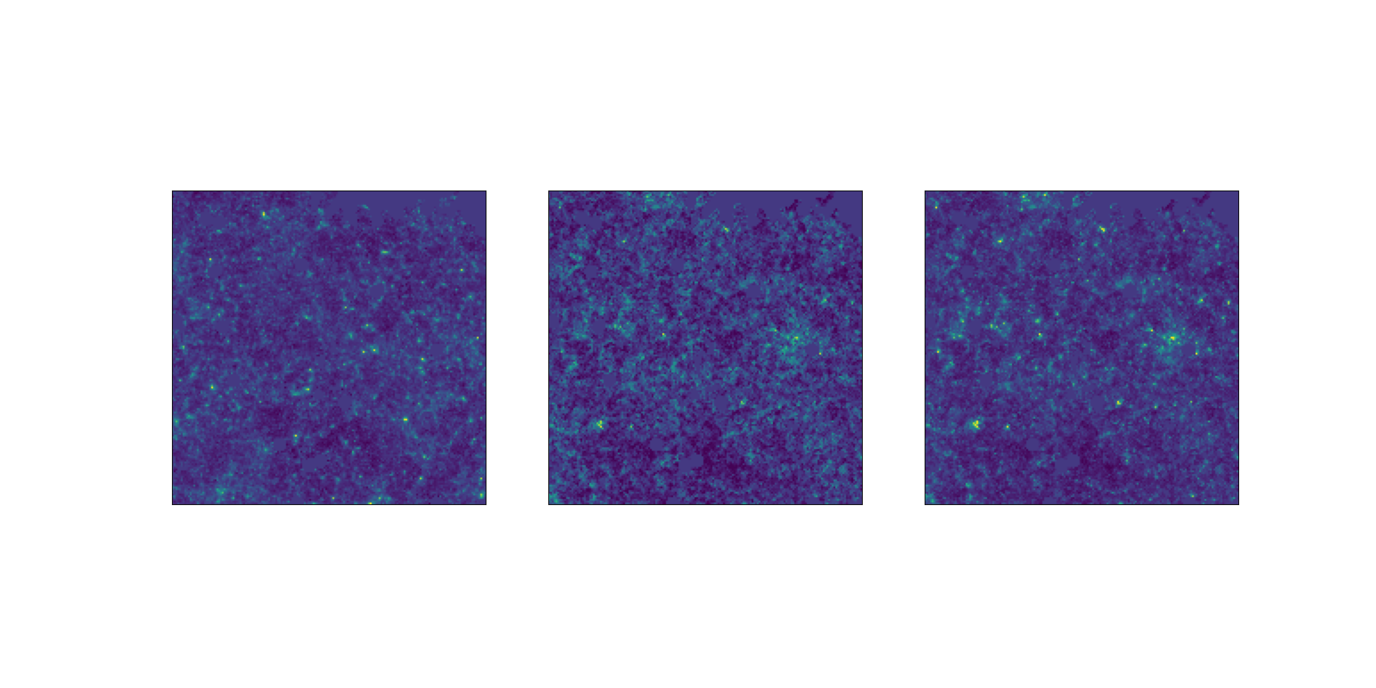
Building more simulations at low cost

LogNormal

Emulated

Challenge simulation

VS

🥳

Zeghal et al. (2025)

Implicit inference with high dimensional data

Implicit inference with high dimensional data

Implicit inference with high dimensional observations is hard

p(x \mid \theta)
  • NLE needs to learn
  • NLE needs to learn
p(\theta \mid x)
  • NPE needs to learn

NF are not good in high dimensions

Goal: to build sufficient statistics as a first step, and then run the NPE or NLE method.

t := f(x)
x

The NF needs to learn the distribution for each     AND the complex relation between     and

x
x
\theta
t := f(x)
x
I(\theta,t)
H(\theta)
H(t)
H(\theta|t)
H(t|\theta)
I(\theta,t) = H(t) - H(t|\theta)
p(\theta \: | \: x) = p(\theta \: | \: f(x)) \Leftrightarrow I(\theta, x) = I(\theta, f(x))

Sufficient Statistic:

Mutual information
Implicit inference with high dimensional data

p(\theta \: | \: x) = p(\theta \: | \: f(x)) \Leftrightarrow I(\theta, x) = I(\theta, f(x))

Sufficient Statistic:

Mutual information

x

Only a matter of the loss function we use!
t := f(x)

Lanzieri & Zeghal et al. (2025)

Implicit inference with high dimensional data
Regression Losses

Information-based Losses

p(\theta \mid x_0)
p(\theta \mid x_1)
p(\theta \mid t = t_0= t_1 =....=t_N)
I(\theta, x) = I(\theta, f(x))
\mathcal{L}_{\text{MIM}} =\underset{f}{\text{ max }} I(\theta, f(x))

→ Build sufficient statistics by definition.

Mean Squared Error (MSE) loss:

\mathcal{L}_{\text{MSE}} = \mathbb{E}_{p(x,\theta)} \left[\parallel \theta - f_\varphi(x) \parallel ^2 \right]

Approximate the mean of the posterior.

p(\theta \: | \: x) = p(\theta \: | \: f(x)) \Leftrightarrow I(\theta, x) = I(\theta, f(x))

Sufficient Statistic:

Implicit inference with high dimensional data
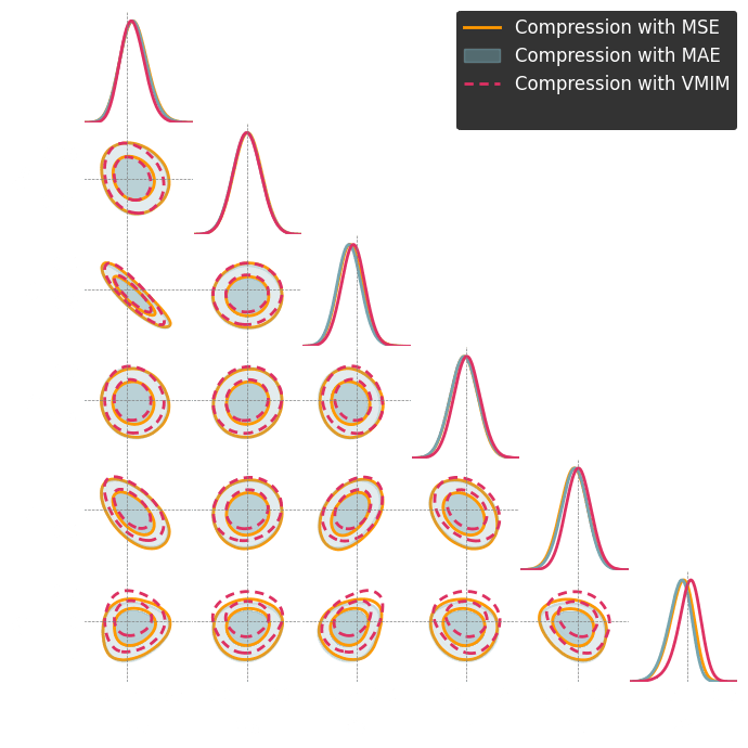
t = f_{\varphi}(x)

Lanzieri & Zeghal et al. (2025)

Implicit inference with high dimensional data
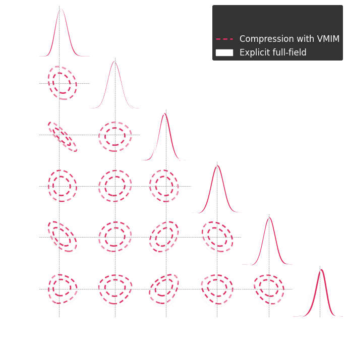
How to validate the inference?

How to validate the inference?

\hat{p}(y\mid x)
p(y\mid x)

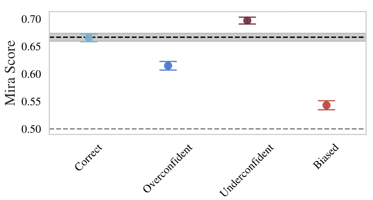
Biased

\hat{p}(y\mid x)
p(y\mid x)

Overconfident

\hat{p}(y\mid x)
p(y\mid x)

Underconfident

Sharief & Zeghal et al. (2026)

How to validate the inference?
\hat{p}(y\mid x)
p(y \mid x)

.

Theorem:

Two distributions are equal if their probability measures are the same over all measurable sets.


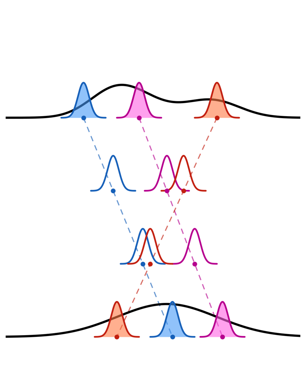
6 pink samples

5 blue samples

6 pink samples

5 blue samples

Sharief & Zeghal et al. (2026)

How to validate the inference?

\hat{p}(y\mid x)
p(y \mid x)

.

Theorem:

Two distributions are equal if their probability measures are the same over all measurable sets.


6 pink samples

5 blue samples

6 pink samples

5 blue samples

6 pink samples

6 pink samples

7 blue samples

Sharief & Zeghal et al. (2026)

How to validate the inference?

\hat{p}(y\mid x)
p(y \mid x)

.

Theorem:

Two distributions are equal if their probability measures are the same over all measurable sets.


6 pink samples

5 blue samples

6 pink samples

5 blue samples

6 pink samples

6 pink samples

7 blue samples

8 pink samples

7 blue samples

Sharief & Zeghal et al. (2026)

How to validate the inference?

\hat{p}(y\mid x)
p(y \mid x)

Theorem:

Two distributions are equal if their probability measures are the same over all measurable sets.


6 pink samples

5 blue samples

6 pink samples

5 blue samples

6 pink samples

6 pink samples

7 blue samples

8 pink samples

7 blue samples

.

Sharief & Zeghal et al. (2026)

How to validate the inference?

\hat{p}(y\mid x)
p(y \mid x)

.

Bayesian approach: what is the probability that the true sample lies inside or outside the region given than n samples from the proposed one are inside?

p(k\mid n)

Theorem:

\text{If } \hat{p}(y \mid x) = p(y \mid x) \text{ then }\: p(k \mid n) \sim Beta(2,1)

Lemma:

\text{If } \hat{p}(y \mid x) = p(y \mid x) \text{ then }
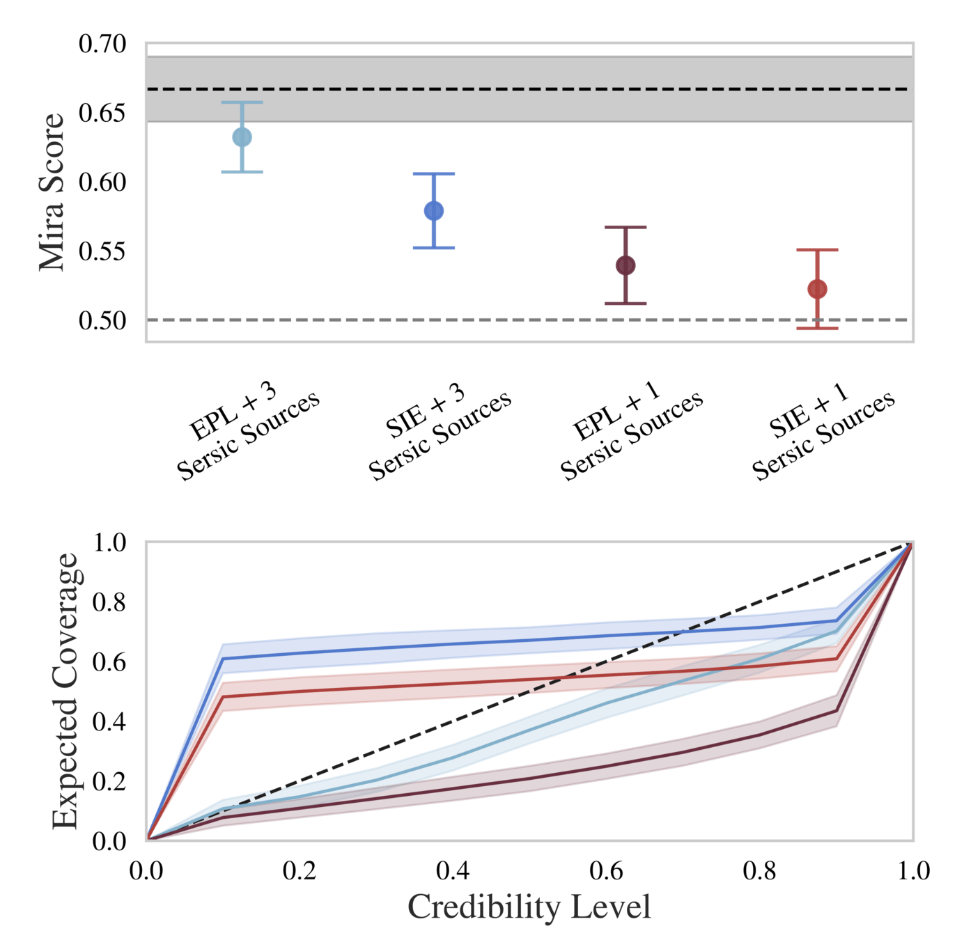
\mu_{Mira} = \mathbb{E}_{p(k,n)}\left[p(k \mid n)\right] = 2/3
= \frac{n+1}{N+2}1_{(k=1)}+ \frac{N-n+1}{N+2}1_{(k=0)}

Sharief & Zeghal et al. (2026)

How to validate the inference?

Is it working?

Check the paper for other examples!

Sharief & Zeghal et al. (2026)

How to validate the inference?

Benefits

  • Sample-based
  • Can work with few samples
  • Works in high dimension
  • Does not rely on training a model
  • Detect miscalibration even when other scores fail
  • It is a scalar value

Which posterior is the best?

Sharief & Zeghal et al. (2026)

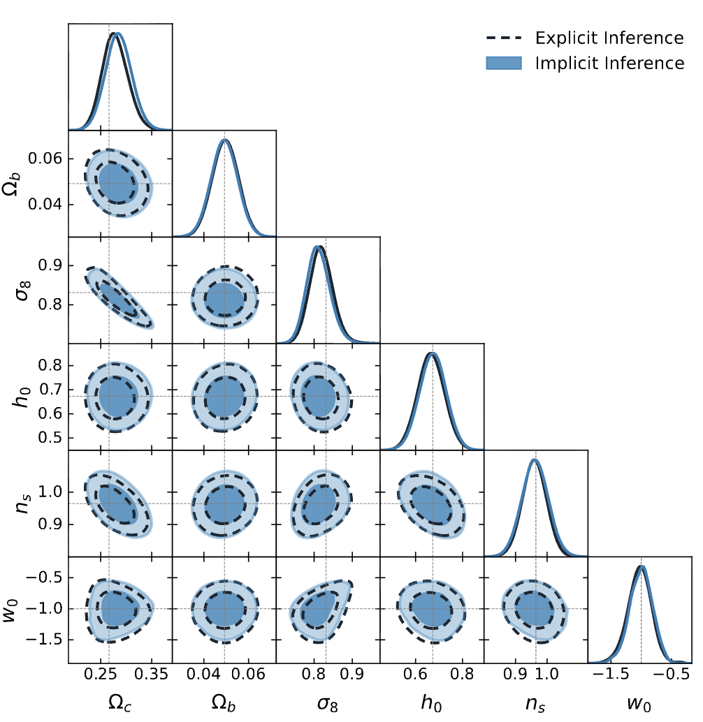
Best validation method: Comparing Explicit and Implicit

Comparing Explicit and Implicit

Omori & Zeghal et al. (2026)

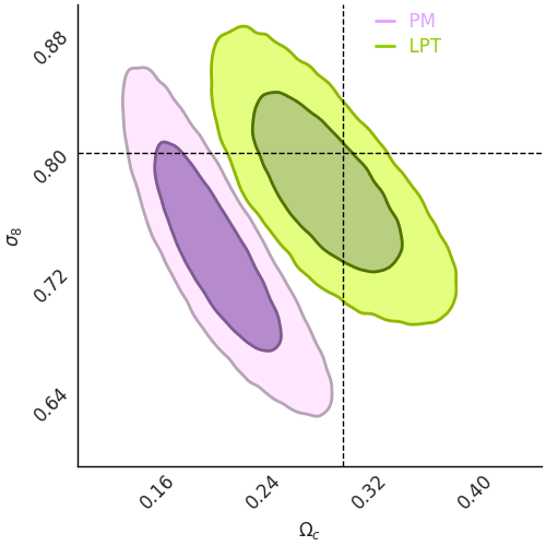
Explicit inference becomes more challenging as the realism (i.e. the complexity) of the simulator increase

In WL: we infer 3D ICs from a 2D field

Before us in WL: only LPT simulators have been used but never validated against implicit
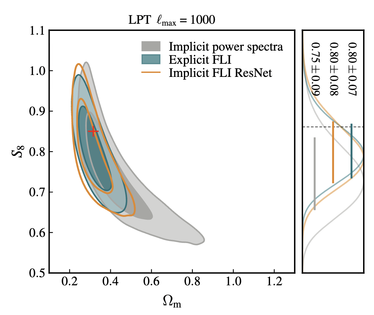
LPT sampling works fine
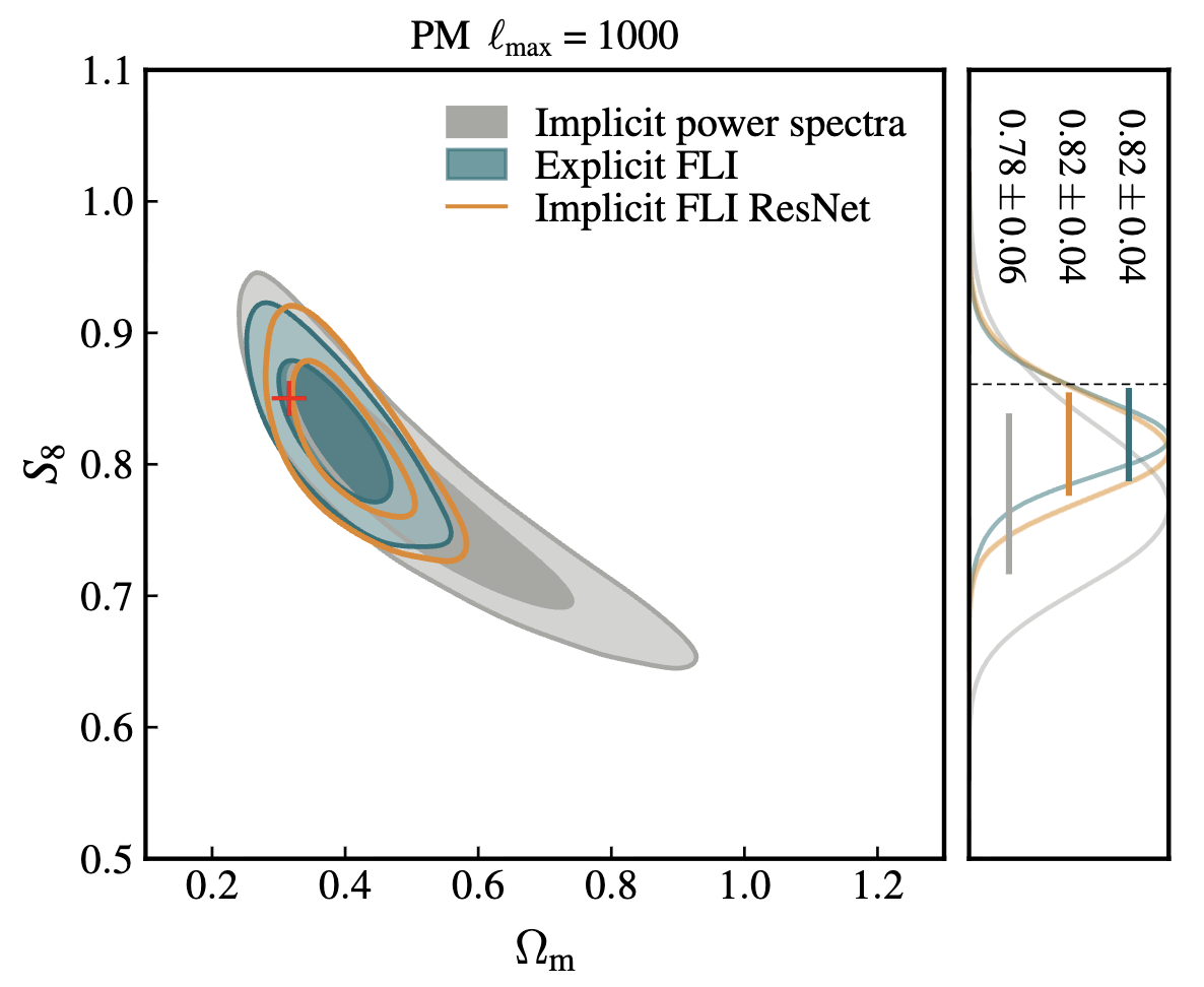
We pushed the comparison to PM Nbody simulators

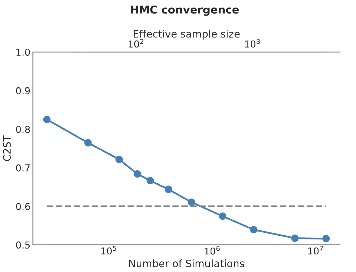
PM sampling works fine but it is very challenging

We need better sampling methods

We need explicit inference methods that can perform with fewer simulations

Zeghal et al. (2024)
Thank you for your attention!