Data Visualization
Karl Ho
School of Economic, Political and Policy Sciences
University of Texas at Dallas
Time series data
-
Time series data
-
Patterns
-
Units
-
Aggregate
-
Discrete data
-
Continuous data
-
Design
-
Discrete
-
Continuous
-
Overview:
-
Trends
-
Cycles/seasonality
-
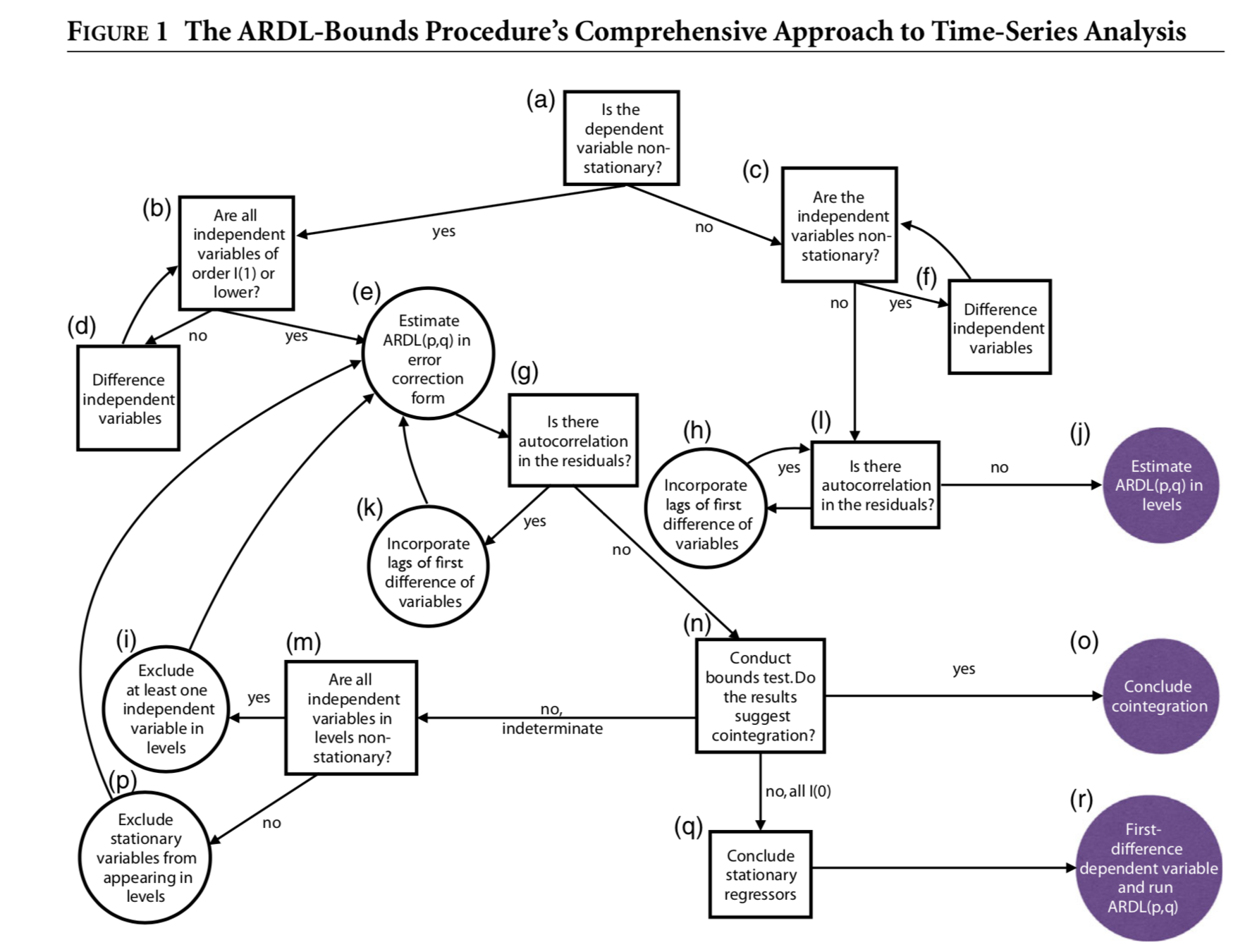
Stationarity
- ARIMA
- Random walk
-
Cointegration
-
"Big picture"
Patterns in time series
Patterns in time series

Patterns in time series
- (d), (h), (i) - Obvious seasonality
- (a), (c), (e), (f) and (i): Trends and changing levels
- (i) Increasing variance also rules out
- (b) and (g): stationary series.
-
Unit of time
-
By day, month or year
-
Irregular measurements (e.g. surveys at different time points)
-
-
Durations
-
Intervals
-
Circularity of time
Attend to:
-
When some data are missing, or irregular measurement points
-
Combine multiple units into higher level units for temporal comparison
-
e.g. day into months, months into year
-
-
Aggregate by
-
Average
-
Counts
-
When to aggregate?
-
"Values are from specific points or blocks of time, and there is a finite number of possible values." (Yau, Ch. 4)
-
X-axis is time points (e.g. month, year)
-
Start the value axis of your bar graph at zero when you’re dealing with all positive values.
-
Barcharts (not histogram)
-
Points (Scatterplot)
-
Discrete time points
-
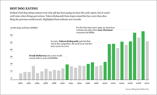
Nathan’s Hot Dog Eating Contest is an annual event that happens every July 4. (Not related to the book's author)
Illustration: Hotdog data barchart

https://en.wikipedia.org/wiki/Nathan%27s_Hot_Dog_Eating_Contest
library(RColorBrewer)
hotdogs <-
  read.csv("http://datasets.flowingdata.com/hot-dog-contest-winners.csv",
           sep=",", header=TRUE)
barplot(hotdogs$Dogs.eaten, names.arg=hotdogs$Year, col="red",
        border=NA, xlab="Year", ylab="Hot dogs and buns (HDB) eaten")
fill_colors <- c()
for ( i in 1:length(hotdogs$Country) ) {
  if (hotdogs$Country[i] == "United States") {
    fill_colors <- c(fill_colors, "grey")
  } else {
    fill_colors <- c(fill_colors, "#2ca25f")
  }
}
barplot(hotdogs$Dogs.eaten, names.arg=hotdogs$Year, col=fill_colors,
        border=NA, xlab="Year", ylab="Hot dogs and buns (HDB) eaten")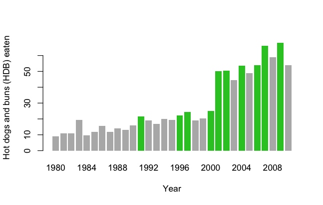
https://en.wikipedia.org/wiki/Nathan%27s_Hot_Dog_Eating_Contest
# Stack bar data
hot_dog_places <-
  read.csv("http://datasets.flowingdata.com/hot-dog-places.csv", sep=",", header=TRUE)
names(hot_dog_places) <- c("2000", "2001", "2002", "2003", "2004",
                           "2005", "2006", "2007", "2008", "2009", "2010")

hot_dog_matrix <- as.matrix(hot_dog_places)
barplot(hot_dog_matrix, border=NA, space=0.25, ylim=c(0, 200),
        xlab="Year", ylab="Hot dogs and buns (HDBs) eaten",
        main="Hot Dog Eating Contest Results, 1980-2010")

# Can this be plotted using ggplot2 stack bar?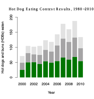
Illustration: Hotdog data barchart
-
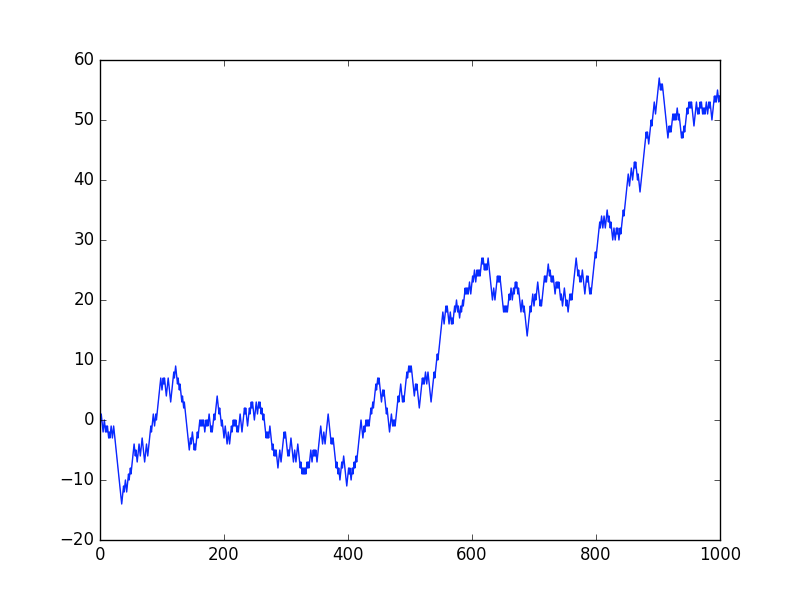
Continuous data can be measured at any time of day during any interval, and it is constantly changing.
-
Better illustrated using point and line charts
-
Note the time units on x axis and limits (upper and lower) of y
Continuous time points
library(quantmod)
library(ggplot2)
library(magrittr)
library(broom)

# Get Apple stock prices
getSymbols("AAPL", src="yahoo")
chartSeries(get("AAPL"), subset='last 4 months')
Illustration: Stock prices

## Plotting multiple series using ggplot2

# Setting time period
start = as.Date("2020-10-01")
end = as.Date("2020-11-10")

# Collect stock names from Yahoo Finance
getSymbols(c("AAPL", "FB", "TSM", "PFE"), src = "yahoo", from = start, to = end)

# Prepare data as xts (time series object)
stocks = as.xts(data.frame(AAPL = AAPL[, "AAPL.Adjusted"],
                           FB = FB[, "FB.Adjusted"],
                           TSM = TSM[, "TSM.Adjusted"],
                           PFE = PFE[, "PFE.Adjusted"]))

# Index by date
names(stocks) = c("Apple", "Facebook", "Taiwan Semiconductor Manu.", "Pfizer")
index(stocks) = as.Date(index(stocks))

# Plot
stocks_series = tidy(stocks) %>%
  ggplot(aes(x=index,y=value, color=series)) +
  geom_line(cex=1) +
  theme_bw()
stocks_series

stocks_series = tidy(stocks) %>%
  ggplot(aes(x=index,y=value, color=series)) +
  geom_line(cex=1) +
  theme_bw() +
  labs(title = "Daily Stock Prices, 10/1/2020 - 11/10/2020",
     subtitle = "End of Day Adjusted Prices",
     caption = "Source: Yahoo Finance") +
  xlab("Date") + ylab("Price") +
  scale_color_manual(values = c("steelblue", "red", "brown","purple")) +
  theme(text = element_text(family = "Apple Garamond"))
Illustration: Stock prices

Showcase:
A. Q. Philips 2018 (AJPS)
Showcase:
A. Q. Philips 2018 (AJPS)
-
ts() in stats
-
forecast
-
TSstudio
-
astsa (Applied Statistical Time Series Analysis) by Shumway and Stoffer
-
dygraphs
-
CRAN Task View: Time Series Analysis
Time series packages in R
-
GitHub: forecast
-
Author: Rob Hyndman
-
Current version:
-
Purpose: Foremost package for automatic time series forecasting.
-
Key Features:
-
auto.arima(): Automatically selects optimal ARIMA model. -
ets(): Exponential smoothing state space model. -
tbats(): Exponential smoothing state space model with Box-Cox transformation. - Includes visualization functions for plotting forecasts
-
Time series packages: forecast
-
GitHub: fable
-
Author: Mitchell O'Hara-Wild
-
Current version: 0.3.3 (CRAN)
-
Purpose: commonly used univariate and multivariate time series forecasting models including exponential smoothing via state space models and automatic ARIMA modelling.
- Key Features:
Time series packages: fable
- GitHub: not active
- Author: Adrian Trapletti, Kurt Hornik, Blake LeBaron
-
Current version: 0.10-54 (CRAN)
-
Purpose: toolkit for time series modeling and hypothesis testing.
-
Key Features:
-
Functions for stationarity tests like adf.test().
-
Time series regression capabilities.
-
ARCH and GARCH modeling functions.
-
-
Sample code:
-
adf.test(diff(AirPassengers))
-
Time series packages: tseries
- GitHub: xts
- Author: Adrian Trapletti, Kurt Hornik, Blake LeBaron
-
Purpose: Managing ordered observations, especially essential for time series data.
-
Key Features:
-
Handles irregular time series with zoo.
-
xts extends zoo to add more powerful time series capabilities.
-
Time-based subsetting and alignment.
-
-
Sample code:
-
z <- zoo(1:10, Sys.Date() + 1:10)
x <- as.xts(z)
-
Time series packages: xts & zoo
- GitHub: not active
- Author: Kung-Sik Chan, Brian Ripley
-
Current version: TSA 1.3.1 (CRAN),
-
Purpose: Primarily used for educational purposes. Offers utilities for time series analysis.
-
Key Features:
-
Time series decomposition.
-
Various hypothesis testing methods.
-
Simulation capabilities.
-
-
Sample code:
-
decomposed <- decompose(AirPassengers)
plot(decomposed)
-
Time series packages: TSA
-
zoo objects are ordered observations stored internally in a vector or matrix with an index attribute
-
zoo is particularly aimed at irregular time series of numeric vectors/matrices, but it also supports regular time series (i.e., series with a certain frequency).
zoo, ts and xts objects
-
ts represents data which has been sampled at equispaced points in time. In the matrix case, each column of the matrix data is assumed to contain a single (univariate) time series.
zoo, ts and xts objects
-
xts objects are matrix objects internally.
-
xts objects are indexed by a formal time object.
-
Most zoo methods work for xts
zoo, ts and xts objects
-
What is S3 system?
- The S3 system in R provides a mechanism for object-oriented programming by allowing functions to exhibit different behaviors depending on the class of the object they operate on (Chambers, 1998).
- This adaptability is at the heart of generic functions in R, such as
print()orplot(), which operate differently based on the type of data passed to them.
S3 Class System in R
- The core principle of S3 is method dispatch. When a generic function is called with an S3 object, R will search for a method that matches the object's class (Wickham, 2019).
-
For example, when using print() with a \(lm\) object (linear model), R dispatches the print.lm function because lm is the class of the object. The process involves:
-
Detecting the class of the object, say "classname".
-
Searching for a method named generic.classname, where "generic" is the generic function's name.
-
Executing the found method, or defaulting to a base method if no class-specific method is found.
-
Method Dispatch
-
Advantages:
-
Flexibility: Easy to extend existing generic functions with new class methods.
-
Simplicity: Offers a straightforward approach to object-oriented programming without the need for formal class definitions.
-
-
Limitations:
-
Informality: Lacks the strict class definitions seen in formal systems like S4, which can lead to less rigorous class structures.
-
Absence of formal inheritance: While some inheritance behavior can be mimicked, S3 lacks a robust inheritance mechanism.
-
Advantages and Limitations
-
The S3 class system provides an intuitive mechanism for object-oriented programming in R, allowing for flexibility in function behaviors based on object classes.
-
Although it lacks the formality of systems like S4, its simplicity and adaptability have made it a staple in the R programming environment.
In a nutshell...
-
The S4 system in R provides a structured mechanism for object-oriented programming, characterized by its strict definitions, formal method dispatch, and support for multiple inheritance (Chambers, 2008). While S3 classes revolve around convention and informality, S4 enforces rigorous class and method definitions.
S4 Class System in R
Key Features
- Formal Class Definitions:
S4 classes have formal definitions, specifying slots (attributes) and their associated classes. - Multiple Inheritance:
S4 supports multiple inheritance, allowing a class to inherit characteristics from several parent classes. - Formal Method Dispatch:
S4 uses a formal method dispatch system based on function signatures, ensuring that methods are called on objects of the correct class. - Validators:
S4 offers the ability to define validation methods for objects, ensuring that objects meet certain criteria.
S4 Class System in R
- Class Definition:
S3: Informal, defined by convention.
S4: Strict, with formal slot definitions. - Method Dispatch:
S3: Dispatch based on the class of the primary argument.
S4: Dispatch based on the signature of all arguments. - Inheritance:
S3: Single inheritance with some informal mechanisms.
S4: Supports multiple inheritance. - Object Creation:
S3: Typically uses lists or vectors, assigned a class by attribute.
S4: Uses the new() function with formal slot assignments.
Compared to S3
- Flexibility vs. Rigidity:
S3: Provides more flexibility, being less formal.
S4: Offers rigidity, ensuring robust class definitions and method dispatch. - Popularity:
S3: More commonly used due to its simplicity and integration with base R functions.
S4: Predominantly used in packages like Bioconductor where strict object definitions are essential.
Compared to S3
The S4 class system in R offers a structured and rigorous approach to object-oriented programming, with clear distinctions from the S3 system. While S4 ensures strict object definitions and robust method dispatch, its complexity makes it less widespread compared to the more accessible and flexible S3 system. However, the choice between S3 and S4 often hinges on the specific requirements of the task at hand.
Conclusion: S3 and S4
Chambers, John M. 1998. Programming with Data. Springer.
Chambers, John .M. 2008. Software for Data Analysis: Programming with R. Springer.
Wickham, Hadley. 2019. Advanced R. CRC Press.
References
- Metcalfe, Andrew V., and Paul S.P. Cowpertwait. 2009. Introductory Time Series with R. New York, NY: Springer New York. http://link.springer.com/10.1007/978-0-387-88698-5 (November 7, 2022).
- Pfaff, Bernhard. 2008. Analysis of Integrated and Cointegrated Time Series with R. 2nd ed. New York: Springer.
- Shumway, Robert H., and David S. Stoffer. 2017. Time Series Analysis and Its Applications: With R Examples. Cham: Springer International Publishing. http://link.springer.com/10.1007/978-3-319-52452-8 (November 7, 2022).
References
-
First specify the goals
-
Trace those goals to the data that are intended to define those goals operationally,
-
Framework for interpreting the data with respect to the stated goals.
It is important to clarify what informational needs the organization has, so that these needs for information can be quantified and analyzed as to whether or not the goals are achieved.
-
Collecting data to serve a purpose
Goal Question Metric (GQM)
-
Simple charts
-
Vertical dimensions showing variables of high importance. The \(y\) dimension is generally viewed as a response, or dependent, variable. the horizontal dimension shows \(x\) or independent variable(s) that affect(s) \(y\).
-
Top-down story: If something is important, it is likely to be important across a large proportion of the data. Thus a design that starts by showing all or most of the data and drills down into different aspects of that overall visualization makes sense for most situations.
Prioritize what's important
-
Milestones in the History of Thematic Cartography, Statistical Graphics, and Data Visualization (http://datavis.ca/milestones/)
-
Graphdrawing.org