Supervised Learning:
Classification

Karl Ho

School of Economic, Political and Policy Sciences

University of Texas at Dallas

Gentle Introduction to Machine Learning

Qualitative variables take values in an unordered set C, such as:

Party ID ∈ {Democrats, Republican, Independent}
Voted ∈ {Yes, No}.

Classification

Given a feature vector X and a qualitative response Y taking values in the set C, the classification task is to build a function C(X) that takes as input the feature vector X and predicts its value for Y ; i.e. C(X) ∈ C.

From prediction point of view, we are more interested in estimating the probabilities that X belongs to each category in C.
For example, voter X will vote for a Republican candidate or will a student credit card owner default.
We cannot exactly say this voter will 100% vote for this party, yet we can say by so much chance she will do so.

Classification

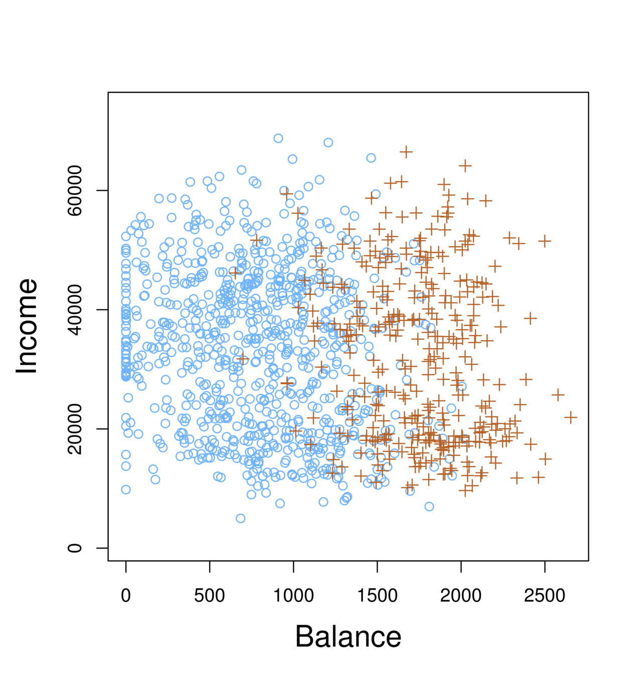
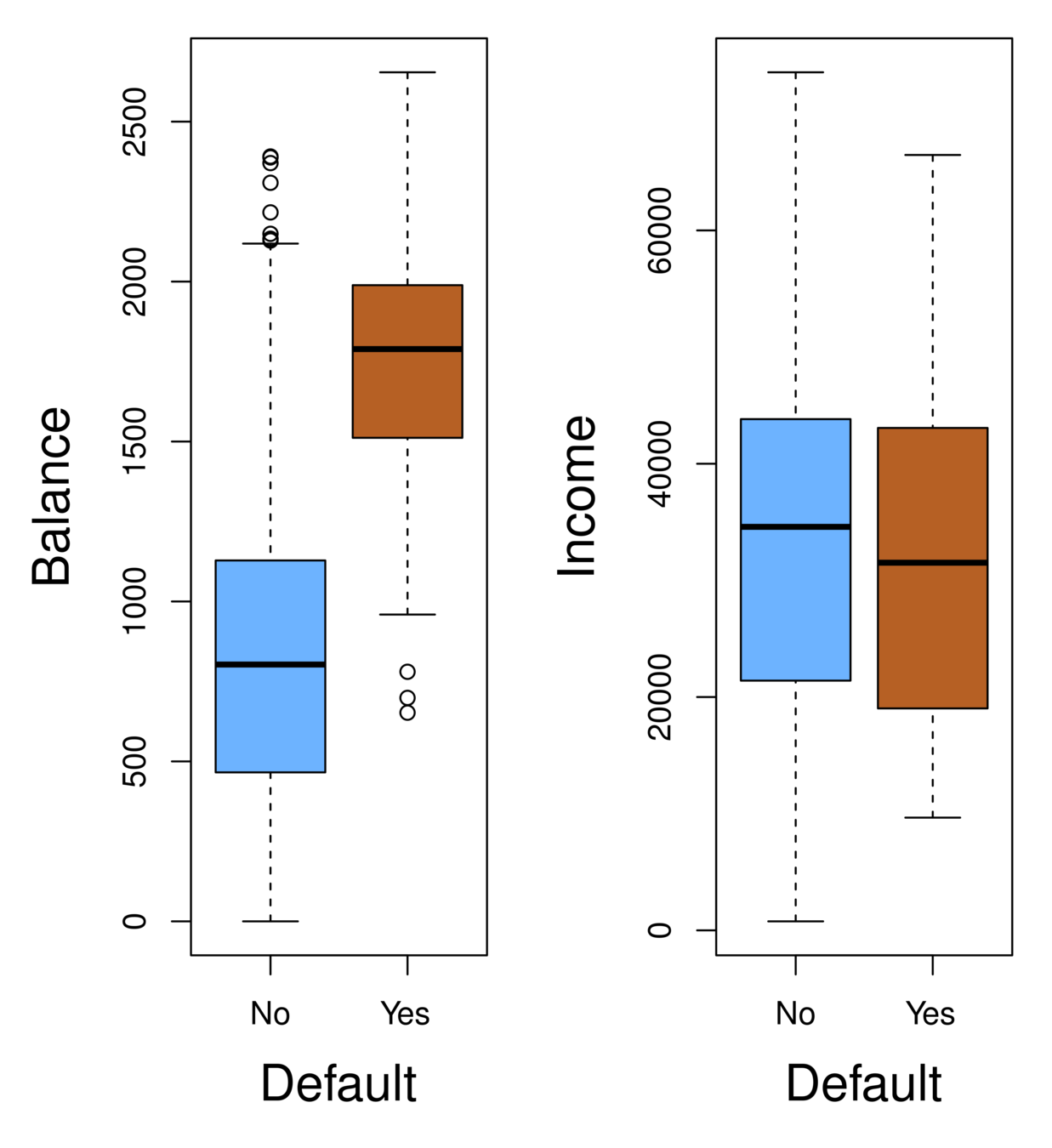
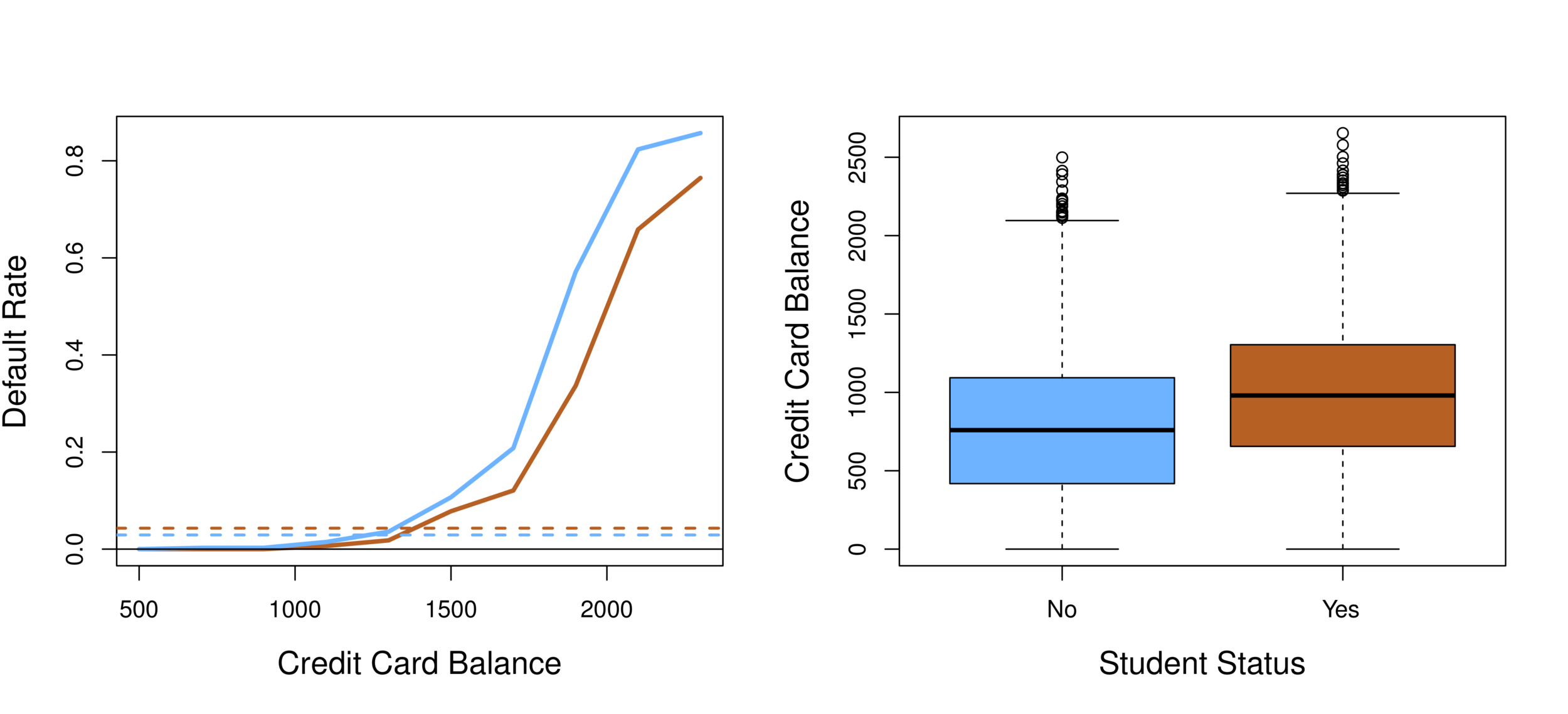
Orange: default, Blue: not
Overall default rate: 3%
Higher balance tend to default

Income has any impact?

Mission:
- Predict default (Y ) using balance (X1) and income (X2).
- Since Y is not quantitative, the simple linear regression model is not appropriate.
- Consider Y being three categories, linear regression cannot be used given the lack of order among these categories.

Classification

Can linear regression be used on two category variable (e.g. 0,1)?
For example, voted (1) or not voted(0), cancer (1) or no cancer (0)
Regression can still generate meaningful results.
Question: What does zero (0) mean? How to assign 0 and 1 to the categories?
For example, Republican and Democrat, pro-choice and pro-life

Classification

Instead of modeling the numeric value of Y responses directly, logistic regression models the probability that Y belongs to a particular category.

Logistic Regression

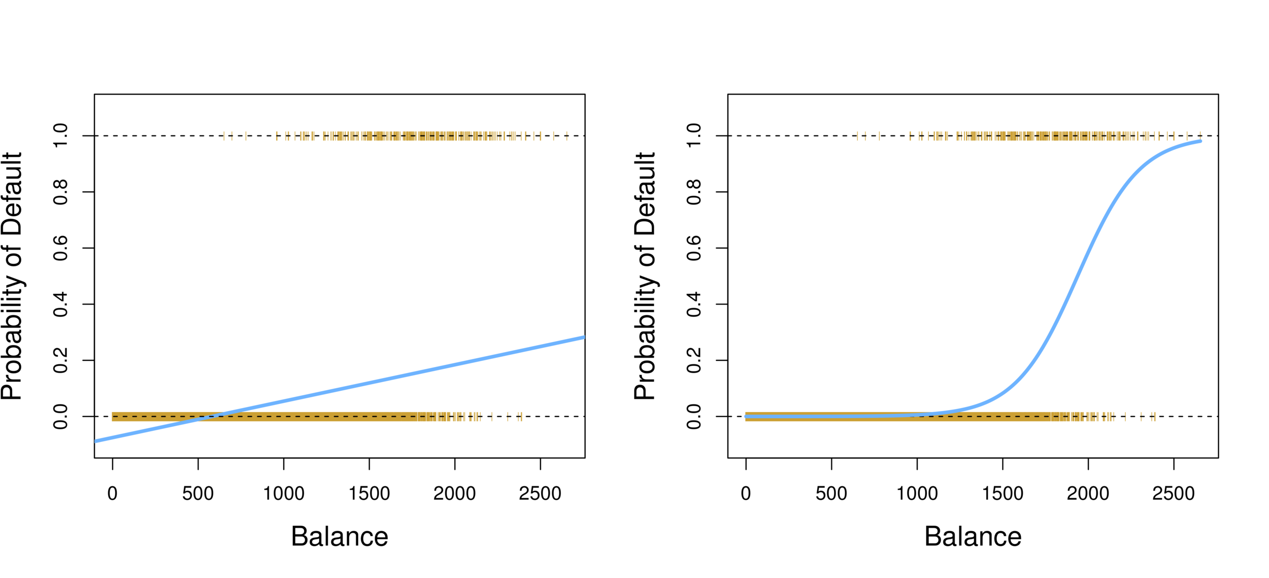
Linear regression vs. Logistic regression
Using linear regression, predictions can go out of bound!

Logistic Regression

Probability of default given balance can be written as:

Pr(default = Yes|balance).
Prediction using p(x)>.5, where x is the predictor variable (e.g. balance)
Can set other or lower threshold (e.g. p(x)>.3

Logistic Regression

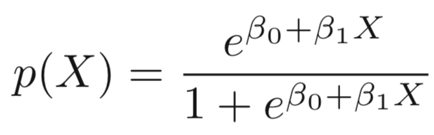
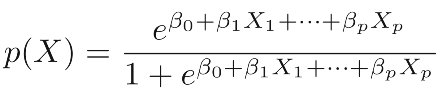
To model p(X), we need a function that gives outputs between 0 and 1 for all values of X.
In logistic regression, we use the logistic function,

Logistic Model

The numerator is called the odds

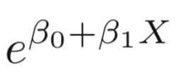
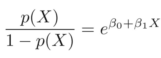
Which is the same as:

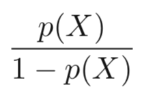
The odds can be understood as the ratio of probabilities between on and off cases (1,0)
For example, on average 1 in 5 people with an odds of 1/4 will default, since p(X) = 0.2 implies an odds of
0.2/(1-0.2) = 1/4.

Logistic Model

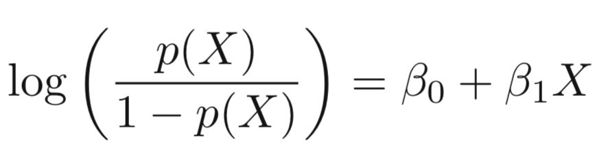
Taking the log of both sides, we have:

Logistic Model

The left-hand side is called the log-odds or logit, which can be estimated as a linear regression with X.
Note that however, p(X) and X are not in linear relationship.

Logistic Regression can be estimated using Maximum Likelihood.
We seek estimates for $\beta_{0}$ and $\beta_{1}$ such that the predicted probability $\hat{p}(x_{i})$ of default for each individual, using
corresponds as closely as possible to the individual’s observed default status.
In other words, we try to find $\beta_{0}$ and $\beta_{1}$such that plugging these estimates into the model for p(X) yields a number close to one (1) for all individuals that fulfill the on condition (e.g. default) and a number close to zero for all individuals of off condition (e.g. not default).

Logistic Regression

Coefficients:
              Estimate Std. Error z value Pr(>|z|)    
(Intercept) -1.065e+01  3.612e-01  -29.49   <2e-16 ***
balance      5.499e-03  2.204e-04   24.95   <2e-16 ***

glm.fit=glm(default~balance,family=binomial)
summary(glm.fit)

Output:

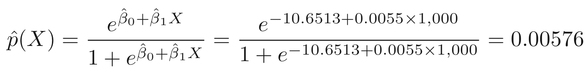
Suppose an individual has a balance of $1,000,

Logistic Regression

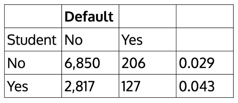
	Default
Student	No	Yes
No	6,850	206	0.029
Yes	2,817	127	0.043

How about the case of students?

> table(student,default)
       default
student   No  Yes
    No  6850  206
    Yes 2817  127

We can actually calculate by hand the rate of default among students:

Logistic Regression

> glm.sfit=glm(default~student,family=binomial)
> summary(glm.sfit)

Coefficients:
            Estimate Std. Error z value Pr(>|z|)    
(Intercept) -3.50413    0.07071  -49.55  < 2e-16 ***
studentYes   0.40489    0.11502    3.52 0.000431 ***

We can extend the Logistic Regression to multiple right hand side variables.

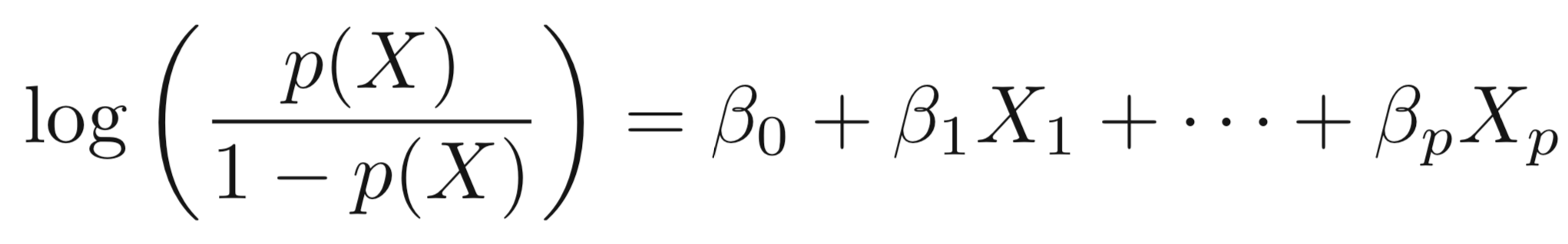
Multiple Logistic Regression

> glm.nfit=glm(default~balance+income+student,data=Default,family=binomial)
> summary(glm.nfit)

Coefficients:
              Estimate Std. Error z value Pr(>|z|)    
(Intercept) -1.087e+01  4.923e-01 -22.080  < 2e-16 ***
balance      5.737e-03  2.319e-04  24.738  < 2e-16 ***
income       3.033e-06  8.203e-06   0.370  0.71152    
student[Yes]  -6.468e-01  2.363e-01  -2.738  0.00619 **

Why student becomes negative? What does this mean?

Multiple Logistic Regression

Confounding effect: when other predictors in model, student effect is different.

Discriminant Analysis

Logistic regression involves directly modeling Pr(Y = k|X = x) using the logistic function. In English, we say that we model the conditional distribution of the response Y, given the predictor(s) X.

This is called the Bayes classifier.

In a two-class problem where there are only two possible response values, say class 1 or class 2, the Bayes classifier corresponds to predicting class 1 if Pr(Y = 1|X = x0) > 0.5 , and class 2 otherwise.

Bayes Theorem

Who is Bayes?

An 18th century English minister who also presented himself as statisticians and philosopher.

His work never was well known until his friend Richard Price found Bayes' notes on conditional probability and got them published.

Lesson to learn: don't tell your friend where you hide your unpublished papers.

~1701-1761

Bayes Theorem

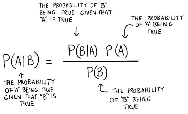
The concept of conditional probability:

Conditional probability is the probability of an event happening, given that it has some relationship to one or more other events.

$$ P(A \mid B) = \frac{P(B \mid A) \, P(A)}{P(B)} $$

To read it, the probability of A given B.

$$ P(A \mid B) = \frac{P(B \mid A) \, P(A)}{P(A)P(B \mid A)+P(\bar{A})P(B \mid \bar{A})} $$

Bayes Theorem

Source: https://www.bayestheorem.net

Bayes Theorem

A prior probability is an initial probability value originally obtained before any
additional information is obtained.

A posterior probability is a probability value that has been revised by using additional
information that is later obtained.

Bayes Theorem

The events must be disjoint (with no overlapping).
The events must be exhaustive, which means that they combine to include all possibilities

Bayes Theorem

The concept of conditional probability:

Conditional probability is the probability of an event happening, given that it has some relationship to one or more other events.

Discriminant Analysis

Suppose that we wish to classify an observation into one of K classes, where
K ≥ 2.

Let $\pi_{k}$ represent the overall or prior probability that a randomly chosen observation comes from the $k^{th}$class; this is the probability that a given observation is associated with the $k^{th}$ category of the response variable Y .

Discriminant Analysis

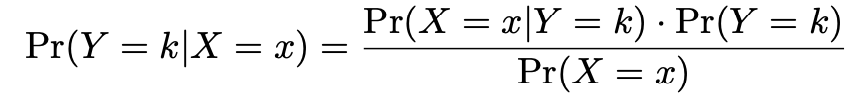
By Bayes theorem:

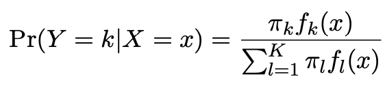
where $\pi_{k}$ = $Pr(Y = k)$ is the marginal or prior probability for class k,

$f_{k}(x)$=$Pr(X=x|Y=k)$ is the density for X in class k. Here we will use normal densities for these, separately in each class.

Discriminant Analysis

We classify a new point according to which density is highest.

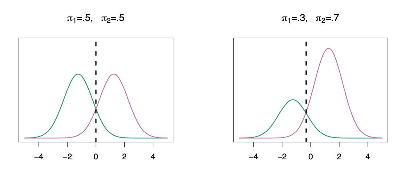
The dashed line is called the Bayes decision boundary.

When the priors are different, we take them into account as well, and compare $\pi_{k}$$f_{k}(x)$. On the right, we favor the pink class — the decision boundary has shifted to the left.

Discriminant Analysis

LDA improves prediction by accounting for the normally distributed x (continuous).

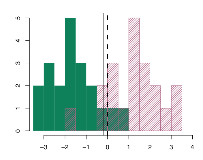
Bayesian decision boundary

LDA decision boundary

Why not linear regression?

Discriminant Analysis

Linear discriminant analysis is an alternative (and better) method:

when the classes are well-separated in multiple-class classification, the parameter estimates for the logistic regression model are surprisingly unstable.
If N is small and the distribution of the predictors X is approximately normal in each of the classes, LDA is more stable.

Discriminant Analysis

Linear discriminant analysis

Dependent variable: categorical
Predictor: continuous + normally distributed

Linear Discriminant Analysis

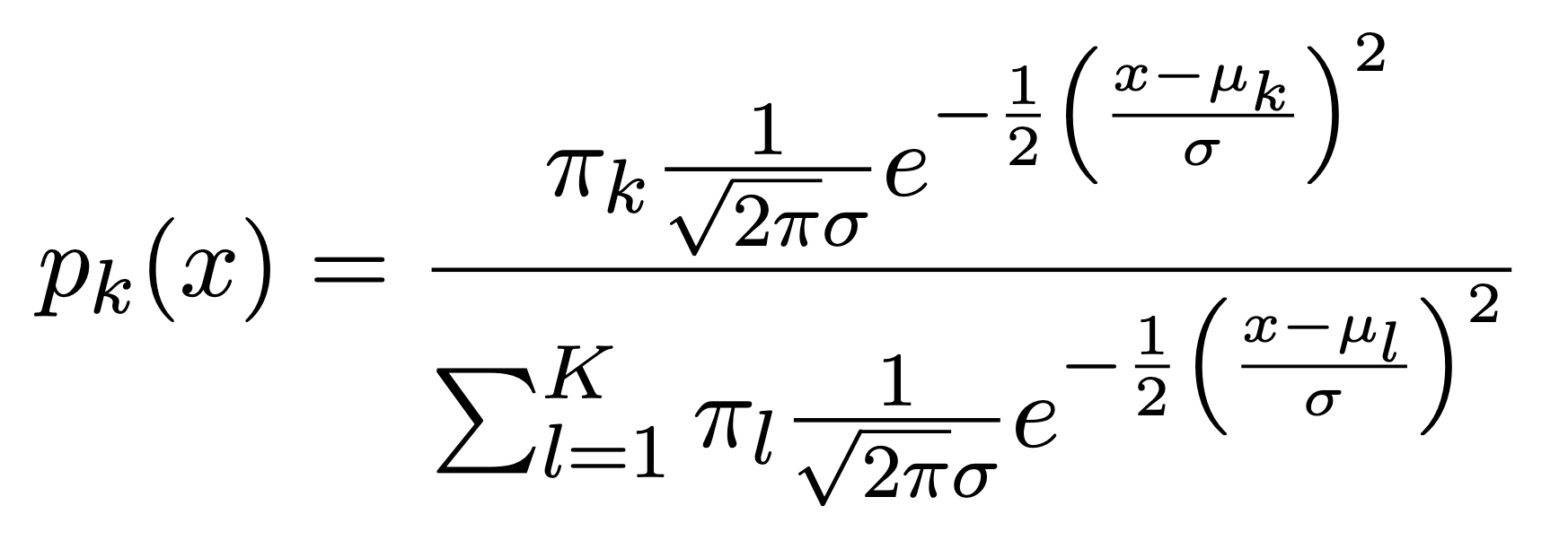
When p=1, The Gaussian density has the form:

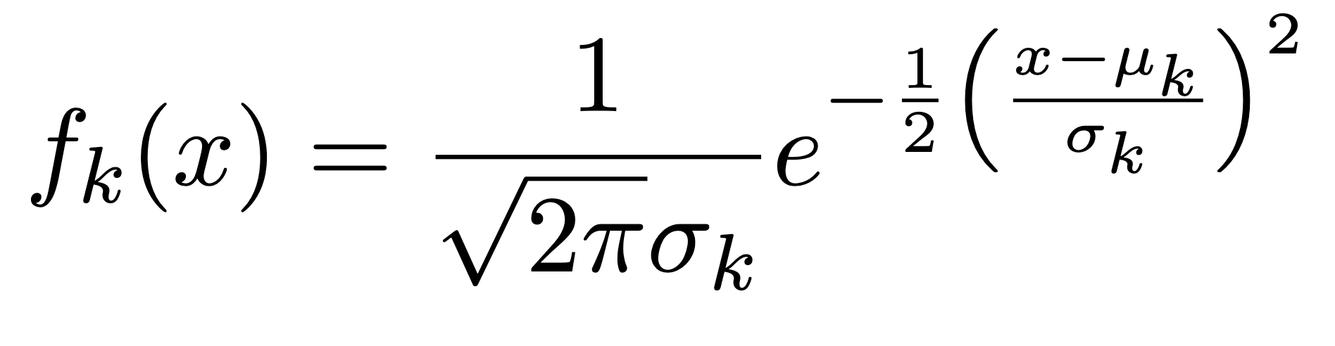
Here $\mu_{k}$ is the mean, and $\sigma_{k}^{2}$ the variance (in class k). We will assume that all the $\sigma_{k}$=$\sigma$are the same. Plugging this into Bayes formula, we get a rather complex expression for $p_{k}(x)$=$Pr(Y=k|X=x)$:

LDA vs. Logistic regression

LDA assumes that the observations are drawn from a Gaussian distribution with a common covariance matrix in each class, and so can provide some improvements over logistic regression when this assumption approximately holds.

Conversely, logistic regression can outperform LDA if these Gaussian assumptions are not met.

Classification methods

Logistic regression is very popular for classification, especially when K = 2.
LDA is useful when n is small, or the classes are well separated, and Gaussian assumptions are reasonable. Also when K > 2.

Confusion matrix: Default data

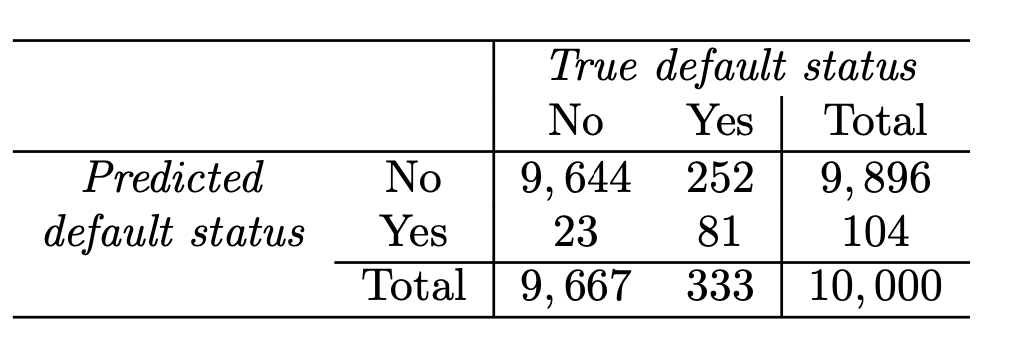
Correct

Incorrect

LDA error: (23+252)/10,000=2.75%

Yet, what matters is how many who actually defaulted were predicted?

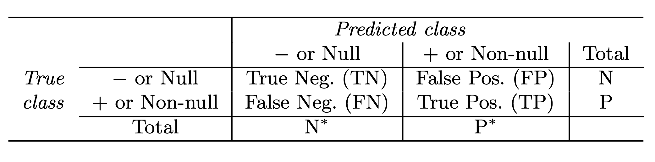
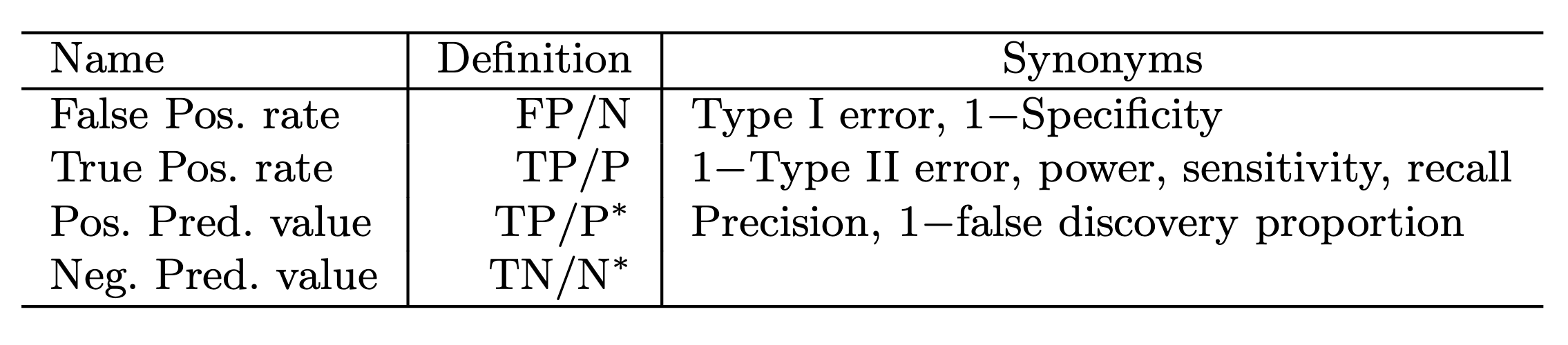
Sensitivity and Specificity

Sensitivity is the percentage of true defaulters that are identified (24.3 % in this case).
Specificity is the percentage of non-defaulters that are correctly identified ( (1 − 23/9, 667) × 100 = 99.8 %.)

Sensitivity and Specificity

The Receiver Operating Characteristics (ROC) curve display the overall performance of a classifier, summarized over all possible thresholds, is given by the area under the (ROC) curve (AUC). An ideal ROC curve will hug the top left corner, so the larger the AUC the better the classifier.

Linear Discriminant Analysis for p >1

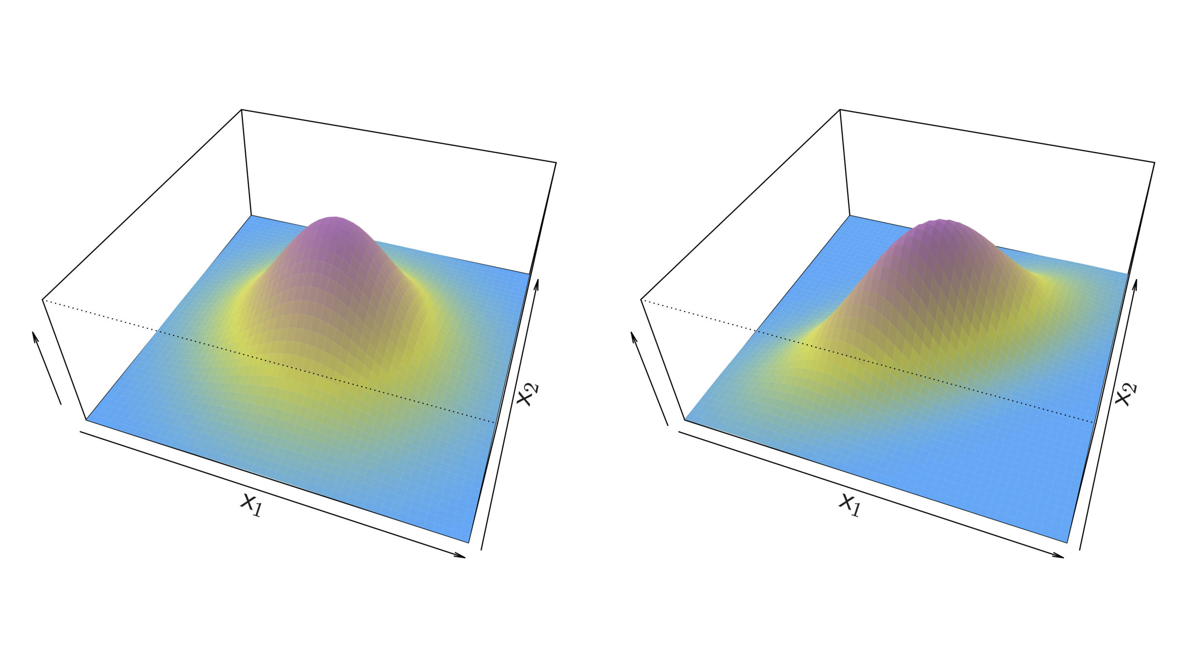
Two multivariate Gaussian density functions are shown, with p = 2. Left: The two predictors are uncorrelated. Right: The two variables have a correlation of 0.7.

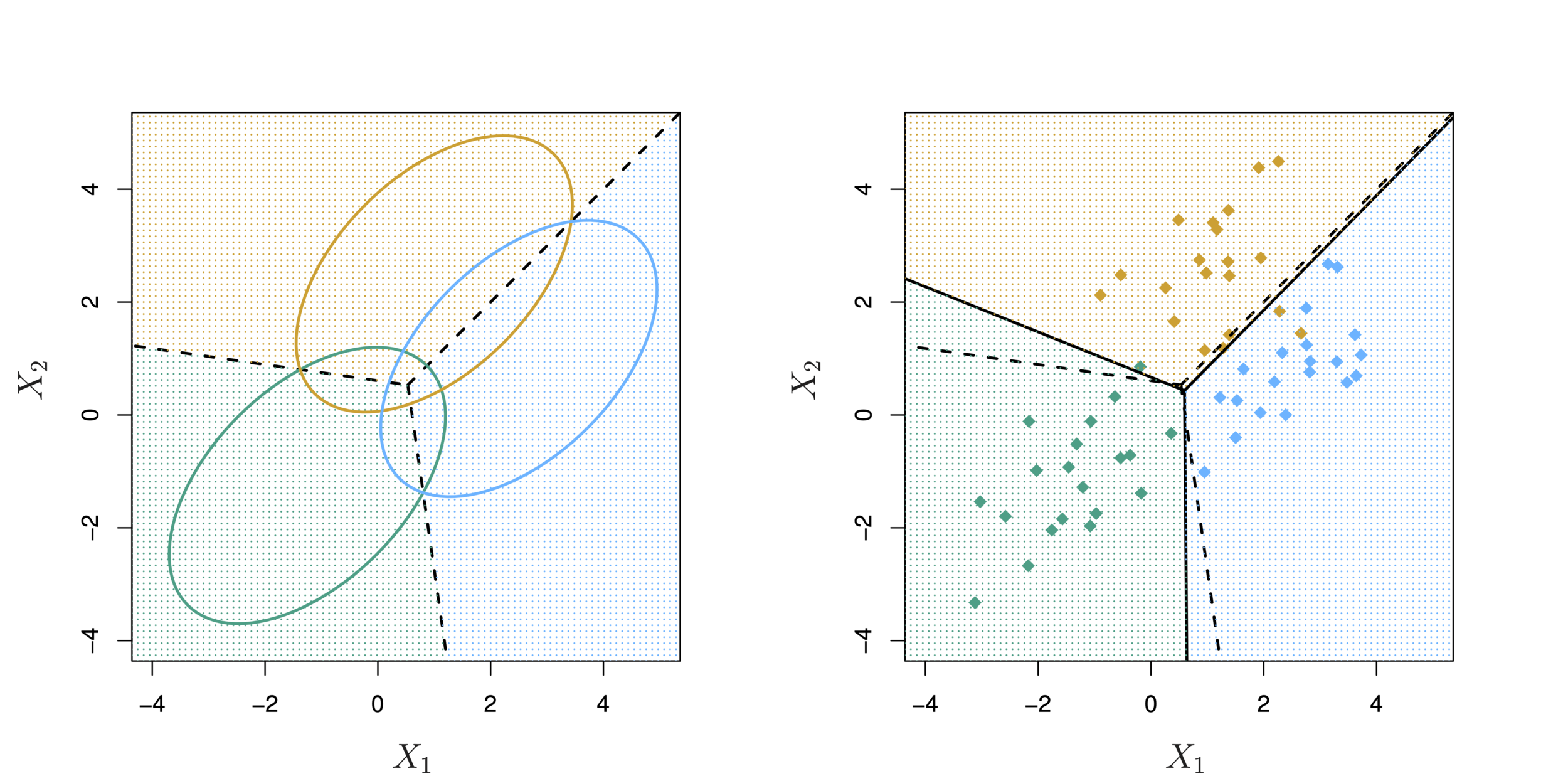
Linear Discriminant Analysis for p >1

LDA with three classes with observations from a multivariate Gaussian distribution(p = 2), with a class-specific mean vector and a common covariance matrix. Left: Ellipses contain 95 % of the probability for each of the three classes. The dashed lines are the Bayes decision boundaries. Right: 20 observations were generated from each class, and the corresponding LDA decision boundaries are indicated using solid black lines.

Supervised Learning: Classification

Gentle Introduction to Machine Learning

Qualitative variables take values in an unordered set C, such as:

Party ID ∈ {Democrats, Republican, Independent}

Voted ∈ {Yes, No}.

Classification

Given a feature vector X and a qualitative response Y taking values in the set C, the classification task is to build a function C(X) that takes as input the feature vector X and predicts its value for Y ; i.e. C(X) ∈ C.

From prediction point of view, we are more interested in estimating the probabilities that X belongs to each category in C.

For example, voter X will vote for a Republican candidate or will a student credit card owner default.

We cannot exactly say this voter will 100% vote for this party, yet we can say by so much chance she will do so.

Classification

Mission:

Predict default (Y ) using balance (X1) and income (X2).

Since Y is not quantitative, the simple linear regression model is not appropriate.

Consider Y being three categories, linear regression cannot be used given the lack of order among these categories.

Classification

Can linear regression be used on two category variable (e.g. 0,1)?

For example, voted (1) or not voted(0), cancer (1) or no cancer (0)

Regression can still generate meaningful results.

Question: What does zero (0) mean? How to assign 0 and 1 to the categories?

For example, Republican and Democrat, pro-choice and pro-life

Classification

Instead of modeling the numeric value of Y responses directly, logistic regression models the probability that Y belongs to a particular category.

Logistic Regression

Logistic Regression

Logistic Regression

Logistic Model

Logistic Model

Logistic Model

Logistic Regression

Logistic Regression

Logistic Regression

Logistic Regression

Multiple Logistic Regression

Multiple Logistic Regression

Multiple Logistic Regression

Discriminant Analysis

Logistic regression involves directly modeling Pr(Y = k|X = x) using the logistic function. In English, we say that we model the conditional distribution of the response Y, given the predictor(s) X.

This is called the Bayes classifier.

In a two-class problem where there are only two possible response values, say class 1 or class 2, the Bayes classifier corresponds to predicting class 1 if Pr(Y = 1|X = x0) > 0.5 , and class 2 otherwise.

Bayes Theorem

Who is Bayes?

An 18th century English minister who also presented himself as statisticians and philosopher.

His work never was well known until his friend Richard Price found Bayes' notes on conditional probability and got them published.

Lesson to learn: don't tell your friend where you hide your unpublished papers.

Bayes Theorem

The concept of conditional probability:

Conditional probability is the probability of an event happening, given that it has some relationship to one or more other events.

$$ P(A \mid B) = \frac{P(B \mid A) \, P(A)}{P(B)} $$

To read it, the probability of A given B.

$$ P(A \mid B) = \frac{P(B \mid A) \, P(A)}{P(A)P(B \mid A)+P(\bar{A})P(B \mid \bar{A})} $$

Bayes Theorem

Bayes Theorem

A prior probability is an initial probability value originally obtained before any additional information is obtained.

A posterior probability is a probability value that has been revised by using additional information that is later obtained.

Bayes Theorem

The events must be disjoint (with no overlapping).

The events must be exhaustive, which means that they combine to include all possibilities

Bayes Theorem

The concept of conditional probability:

Conditional probability is the probability of an event happening, given that it has some relationship to one or more other events.

Discriminant Analysis

Suppose that we wish to classify an observation into one of K classes, where K ≥ 2.

Let \(\pi_{k}\) represent the overall or prior probability that a randomly chosen observation comes from the \(k^{th}\)class; this is the probability that a given observation is associated with the \(k^{th}\) category of the response variable Y .

Discriminant Analysis

By Bayes theorem:

where \(\pi_{k}\) = \(Pr(Y = k)\) is the marginal or prior probability for class k,

\(f_{k}(x)\)=\(Pr(X=x|Y=k)\) is the density for X in class k. Here we will use normal densities for these, separately in each class.

Discriminant Analysis

Discriminant Analysis

Discriminant Analysis

Linear discriminant analysis is an alternative (and better) method:

when the classes are well-separated in multiple-class classification, the parameter estimates for the logistic regression model are surprisingly unstable.

If N is small and the distribution of the predictors X is approximately normal in each of the classes, LDA is more stable.

Discriminant Analysis

Linear discriminant analysis

Dependent variable: categorical

Predictor: continuous + normally distributed

Linear Discriminant Analysis

LDA vs. Logistic regression

Supervised Learning:
Classification

A prior probability is an initial probability value originally obtained before any
additional information is obtained.

A posterior probability is a probability value that has been revised by using additional
information that is later obtained.

Suppose that we wish to classify an observation into one of K classes, where
K ≥ 2.