Supervised Learning: Regression
Karl Ho
School of Economic, Political and Policy Sciences
University of Texas at Dallas
Gentle Introduction to Machine Learning
Overview
-
Linear Regression
-
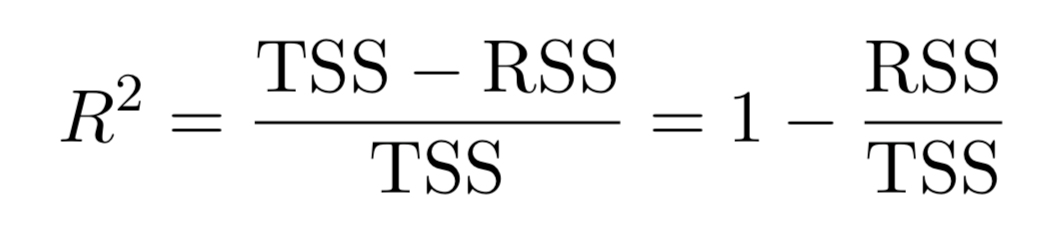
Assessment of regression models
-
Multiple Linear Regression
-
Four important questions
-
Selection methods
-
Qualitative variables
-
Interaction terms
-
Nonlinear effects
Linear regression is a simple approach to supervised learning based on the assumption that the dependence of \(Y\) on \(X_{i}\) is linear.
True regression functions are never linear!
Real data are almost never linear due to different types of errors:
-
measurement
-
sampling
-
multiple covariates
Despite its simplicity, linear regression is very powerful and useful both conceptually and practically.
If prediction is the goal, how we can develop a synergy out of these data?
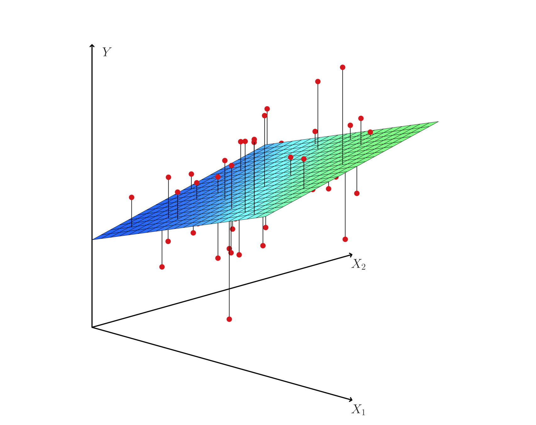
Hyperplane: multiple (linear) regression
Given some estimates \(\hat{\beta_{0}}\) and \(\hat{\beta_{1}}\) for the model coefficients, we predict dependent variable using:
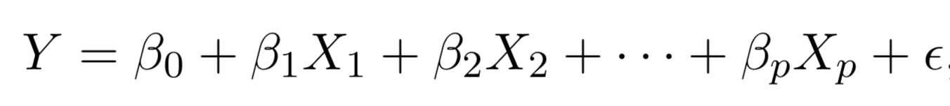
\(Y\) = \(\beta_{0}\) + \(\beta_{1}\)\(X\) + \(\epsilon\)
where \(\beta_{0}\) and \(\beta_{1}\) are two unknown constants that represent the intercept and slope, also known as coefficients or parameters, and \(\epsilon\) is the error term.
\(\hat{y}\) = \(\hat{\beta_{0}}\) + \(\hat{\beta_{1}}\)\(x\)
Assume a model:
Given some estimates \(\hat{\beta_{0}}\) and \(\hat{\beta_{1}}\) for the model coefficients, we predict the dependent variable using:
where \(\hat{y}\) indicates a prediction of Y on the basis of X = x. The hat symbol denotes an estimated value.
\(\hat{y}\) = \(\hat{\beta_{0}}\) + \(\hat{\beta_{1}}\)\(x\)
\(\hat{y}\) = \(\hat{\beta_{0}}\) + \(\hat{\beta_{1}}\)\(x\)
Where is the \(e\)?
The least squares approach chooses \(\hat{\beta_{0}}\) and \(\hat{\beta_{1}}\) to minimize the RSS.
• Let \(\hat{y}_{i}\) = \(\hat{\beta_{0}}\) + \(\hat{\beta_{1}}\)\(x_{i}\) be the prediction for Y based on the \(i^{th}\) value of X. Then \(e_{i}\)=\(y_{i}\)-\(\hat{y}_{i}\) represents the \(i^{th}\) residual
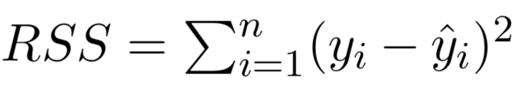
• We define the residual sum of squares (RSS) as:
Estimation of the parameters by least squares
\(RSS\) = \(e_{1}^{2}\) + \(e_{2}^{2}\) + · · · + \(e_{n}^{2}\),
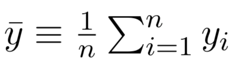
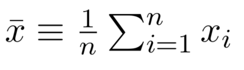
where and
are the sample means.
The least squares approach chooses βˆ0 and βˆ1 to minimize the RSS. The minimizing values can be shown to be:
Estimation of the parameters by least squares

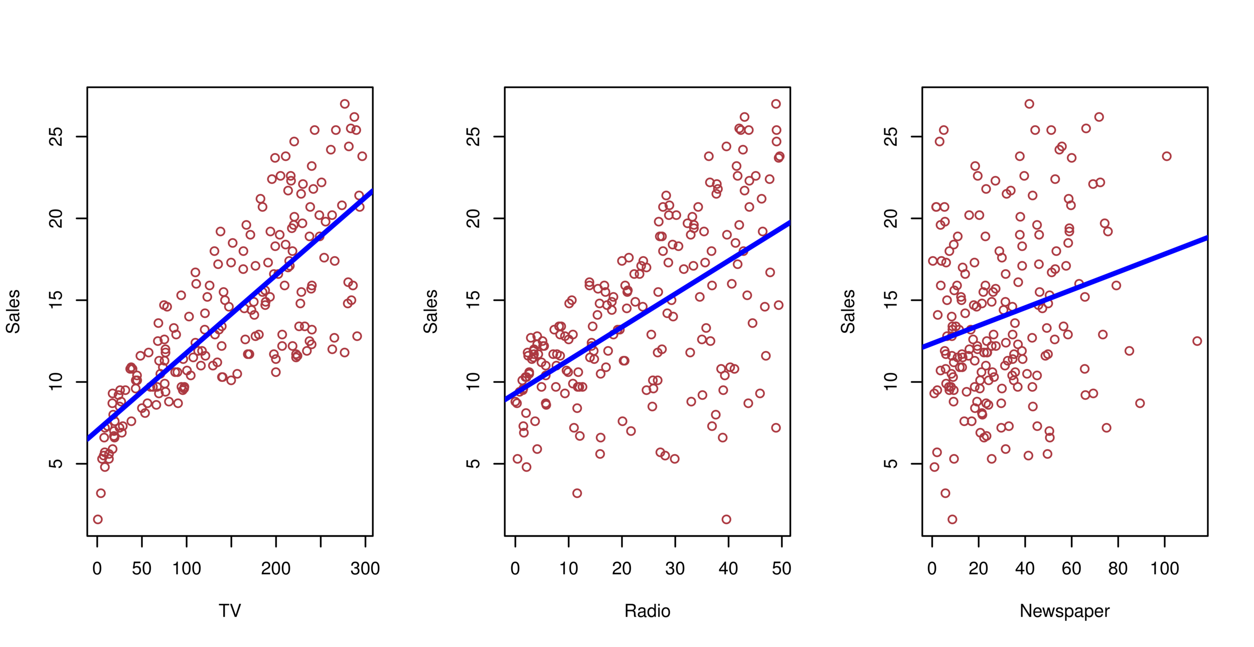
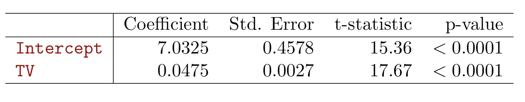
Advertising example
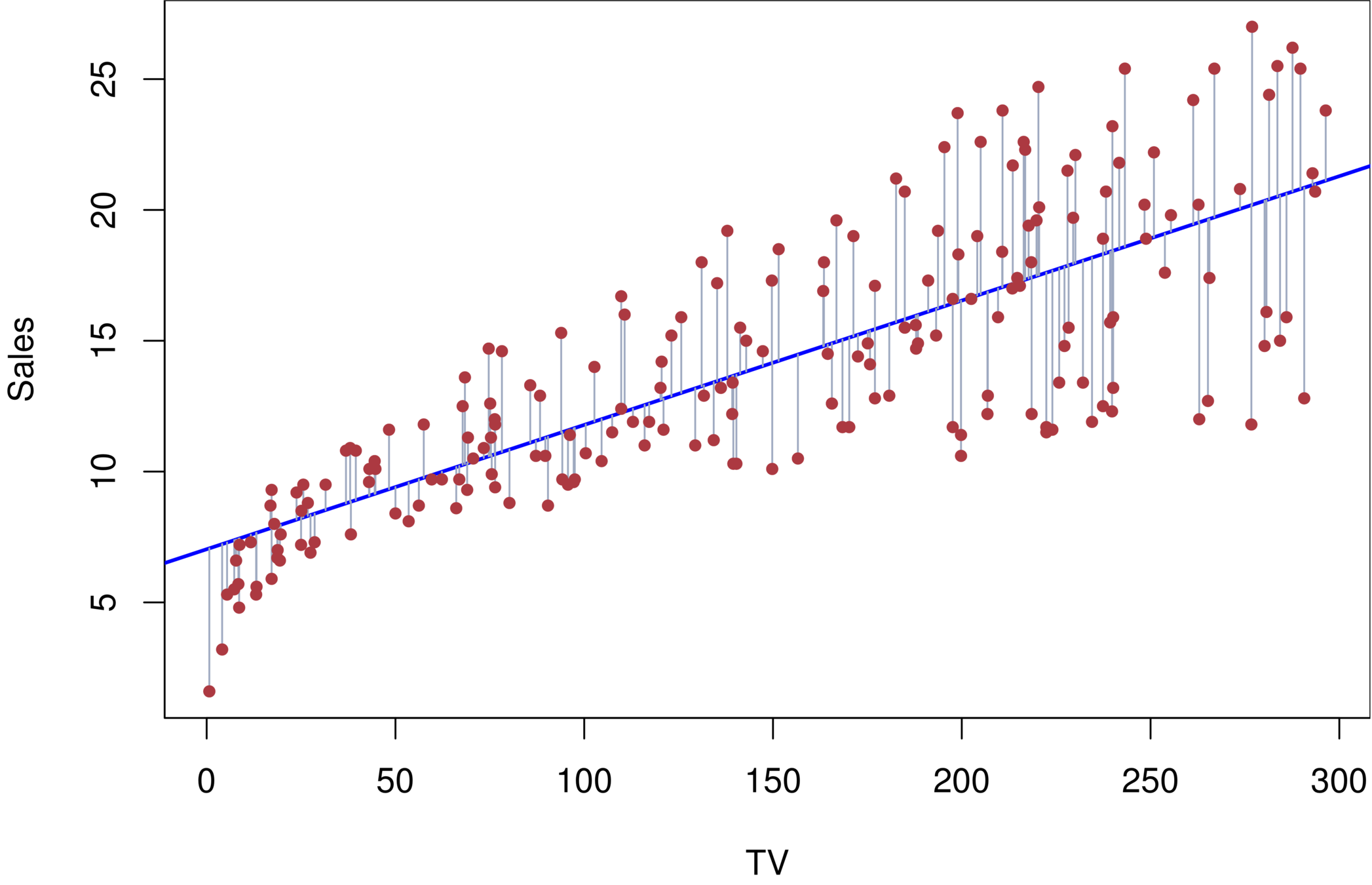
The least squares fit for the regression of sales onto TV. In this case a linear fit captures the essence of the relationship.
Assessment of regression model
-
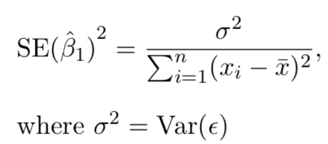
Standard errors
-
Using \(se\) and estimated coefficients, statistics such as t can be calculated for statistical significance:
-
\(t\)=\(\beta\)/\(se\)
-
Assessment of regression model
Standard errors can be used to compute confidence intervals. A 95% confidence interval is defined as a range of values such that with 95% probability, the range will contain the true unknown value of the parameter. It has the form:
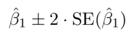
Confidence interval are important for both frequentists and Bayesians to determine a predictor is "significant" or important in predicting y
Assessment of regression model
Assessment of regression model
Assessment of regression model
Model fit:
-
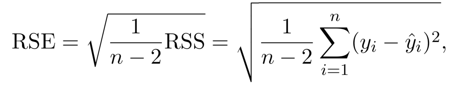
Residual Standard Error (RSS)
Multiple Linear regression
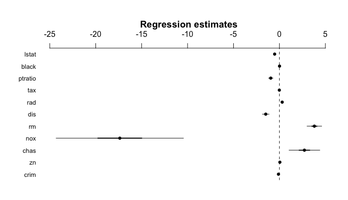
Multiple regression extends the model to multiple \(X\)'s or \(X_{p}\) where \(p\) is the number of predictors.
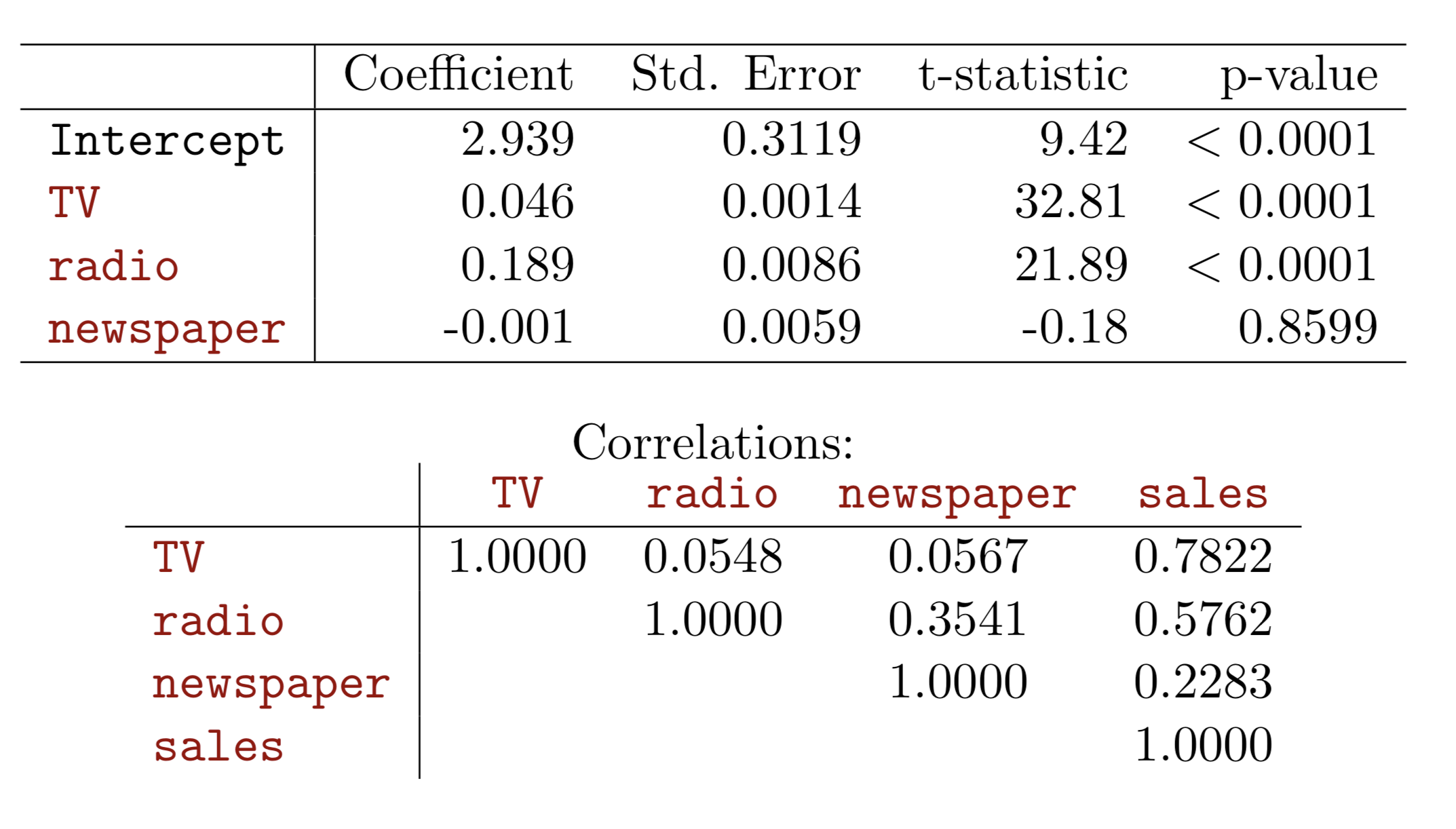
We interpret \(\beta_{j}\) as the average effect on Y of a one unit increase in \(X_{j}\), holding all other predictors fixed. In the advertising example, the model becomes:

-
Each coefficient is estimated and tested separately, provided that there is no correlations among \(X\)'s
-
Interpretations such as “a unit change in \(X_{j}\) is associated with a \(\beta_{j}\) change in \(Y\) , while all the other variables stay fixed”, are possible.
-
Correlations amongst predictors cause problems:
-
The variance of all coefficients tends to increase, sometimes dramatically
-
Interpretations become hazardous — when \(X_{j}\)changes, everything else changes.
-
Multiple Linear regression
-
Problem of Multicollinearity
-
Claims of causality should be avoided for observational data.
Multiple Linear regression
Hyperplane: multiple (linear) regression
Multiple (linear) regression
Advertising example
-
Is at least one of the predictors \(X_1 , X_2 , . . . , X_p\) useful in predicting the response?
-
Do all the predictors help to explain Y, or is only a subset of the predictors useful?
-
How well does the model fit the data?
-
Given a set of predictor values, what response value should we predict, and how accurate is our prediction?
Four important questions
-
F-statistic to determine if at least one of the predictor's coefficient \(\beta_i\) is zero.
-
When there is a very large number of variables \((p > n)\), F-statistic cannot be used.
-
Can consider variable selection methods.
1. Is there a relationship between the response and predictors?
-
There are a total of \(2^p\) models that contain subsets of \(p\) variables.
- For example, when \(p=2\), there will be \(2^2=4\) models.
- model(1) with no variables
- model(2) with \(X_1\) only
- model(3) with \(X_2\) only
- model(4) with both \(X_1\) and \(X_2\).
- For example, when \(p=2\), there will be \(2^2=4\) models.
- When \(p\) becomes large, we need to consider variable selection methods:
- Forward selection: start with null model and add variable with lowest RSS then forward
- Backward selection: start with full model then remove variable with biggest p-value
- Mixed selection: start with null first forward then backward
2. Deciding on Important Variables
- Residual Standard Error (RSE) and \(R^2\), the fraction of variance explained can be used for model fit. The lower of RSE, the better. The higher the \(R^2\), the better.
- More predictors may not be always better. (e.g. Advertising example)
- Linear assumption is tested.
- Graphical analysis will help identifying more subtle relationship in different combination of RHS variables including interaction terms.
3. Model fit
3. Model fit

3. Model fit
- From the pattern of the residuals, we can see that there is a pronounced non-linear relationship in the data.
- The positive residuals (those visible above the surface), tend to lie along the 45-degree line, where TV and Radio budgets are split evenly.
- The negative residuals (most not visible), tend to lie away from this line, where budgets are more lopsided.
-
Three kinds of uncertainties
-
Reducible error: inaccurate coefficient estimates
-
Confidence intervals can be used.
-
-
Model bias: linearity assumption tested
-
Irreducible error: random error \(\epsilon\) in the model
-
Prediction intervals
-
Prediction intervals are always wider than confidence intervals, because they incorporate both the error in the estimate for \(f(X)\) (the reducible error) and the uncertainty as to how much an individual point will differ from the population regression plane (the irreducible error).
-
-
4. Prediction
With current computation power, we can test all subsets or combinations of the predictors in the regression models.
It will be costly, since there are \(2^{p}\) of them; it could be hitting millions or billions of models!
New technology or packages have been developed to perform such replicative modeling.
A Stata package mrobust by Young & Kroeger (2013)
What are important?
-
Begin with the null model — a model that contains an intercept but no predictors.
-
Fit \(p\) simple linear regressions and add to the null model the variable that results in the lowest RSS.
-
Add to that model the variable that results in the lowest RSS amongst all two-variable models.
-
Continue until some stopping rule is satisfied, for example when all remaining variables have a p-value above some threshold.
Selection methods: Forward selection
-
Start with all variables in the model.
-
Remove the variable with the largest p-value, that is, the variable that is the least statistically significant.
-
The new (\(p\) − 1)-variable model is fit, and the variable with the largest p-value is removed.
-
Continue until a stopping rule is reached. For instance, we may stop when all remaining variables have a significant p-value defined by some significance threshold.
Selection methods: backward selection
-
Mallow’s \(C_{p}\)
-
Akaike information criterion (AIC)
-
Bayesian information criterion (BIC)
-
Cross-validation (CV).
New selection methods
-
Categorical variables
-
Dichotomy (1,0)
-
class (1,2,3)
-
Leave one category as base category for comparison:
-
e.g. race, party
-
-
Qualitative variables
-
Treatment of two highly correlated variables
-
Multiplicative term--> Interaction term
-
Useful for multicollinearity problem
-
Hard to interpret and could lead to other problems
-
Hierarchy principle:
If we include an interaction in a model, we should also include the main effects, even if the p-values associated with their coefficients are not significant.
Interaction term/variables
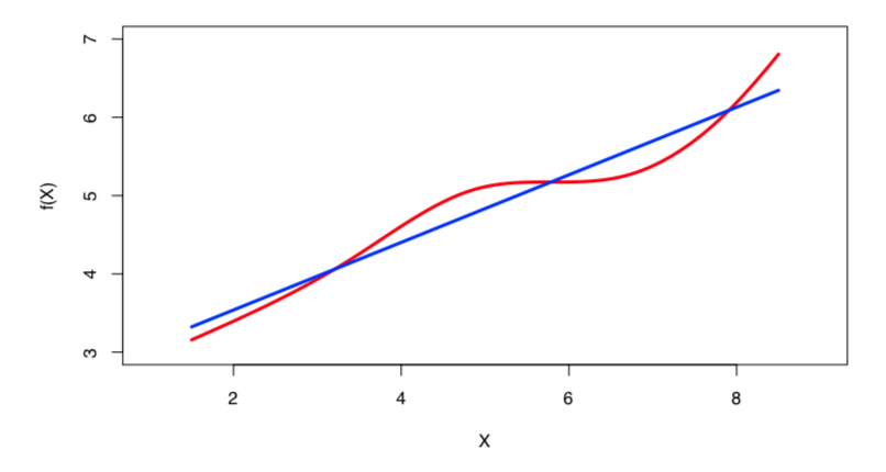
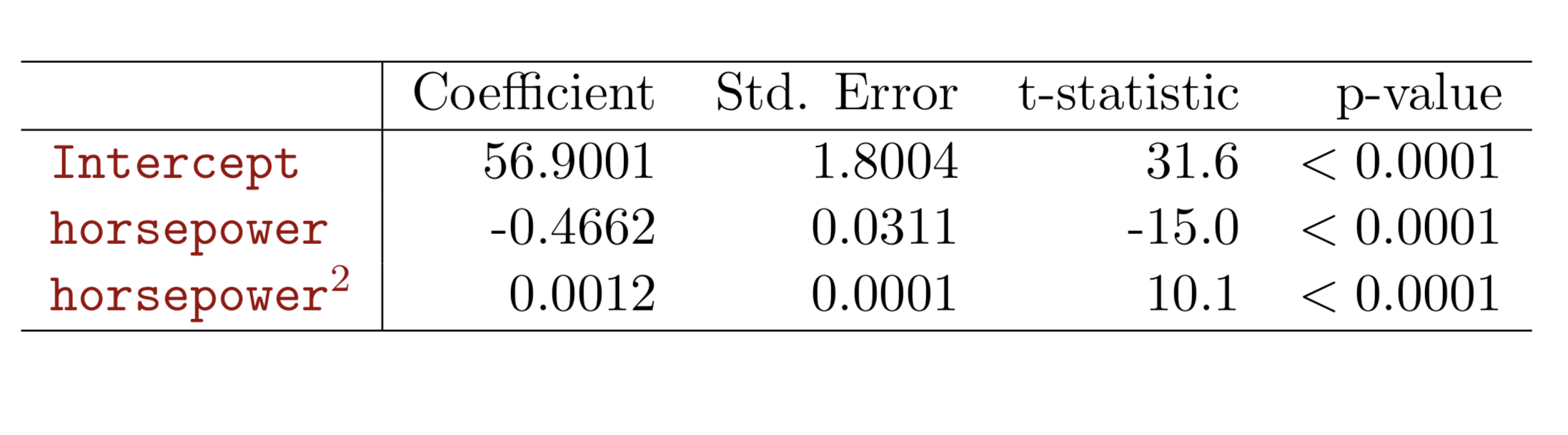
Nonlinear effects
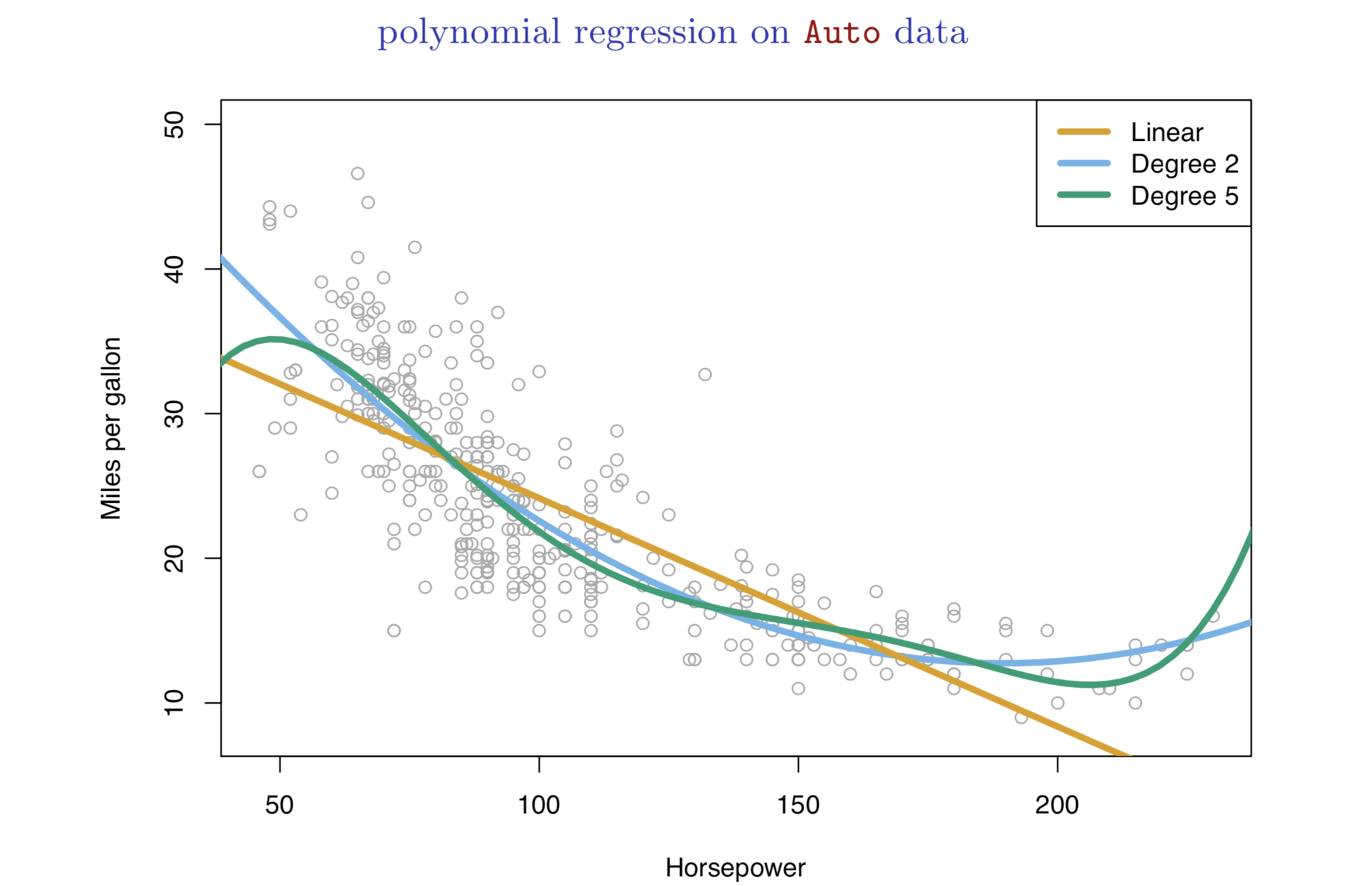
Nonlinear effects

-
Linear regression is a good starting point for predictive analytics
-
Simple
-
Highly interpretable
-
Error management
-
-
Limitations:
-
Numeric, quantitative variables
-
Need clear interpretations
-
other problems of regression?
-
-
Next: Classification and tree-based methods